Absorption, Emission, and Scattering in Spectroscopy: A Guide for Pharmaceutical Scientists

Abstract

This article provides a comprehensive guide to the fundamental principles and practical applications of absorption, emission, and scattering phenomena in spectroscopy. Tailored for researchers and drug development professionals, it explores the theoretical underpinnings of light-matter interactions, details methodological approaches for pharmaceutical analysis, addresses common troubleshooting scenarios, and offers a comparative framework for technique selection. By integrating foundational science with real-world applications, this resource aims to enhance analytical capabilities in drug discovery, formulation, and quality control, supporting the advancement of both small-molecule and biologic therapies.

Core Principles: How Light Interacts with Matter in Pharmaceutical Analysis

Electromagnetic radiation is a form of energy that exhibits properties of both waves and particles, and its behavior is fundamental to spectroscopic analysis [1]. It consists of oscillating electric and magnetic fields that propagate through space, characterized by key properties such as velocity, amplitude, frequency, and wavelength [1]. The entire electromagnetic spectrum is organized by frequency or wavelength, divided into separate bands including radio waves, microwaves, infrared, visible light, ultraviolet, X-rays, and gamma rays [2]. Throughout most of this spectrum, spectroscopy serves as the primary technique to separate waves of different frequencies, measuring radiation intensity as a function of frequency or wavelength to study interactions between electromagnetic waves and matter [2].

The energy of electromagnetic radiation is directly proportional to its frequency and inversely proportional to its wavelength, as described by the equation ( E = hf = \frac{hc}{\lambda} ), where ( h ) is Planck's constant, ( c ) is the speed of light, ( f ) is frequency, and ( \lambda ) is wavelength [1] [2]. This relationship is crucial for understanding how different regions of the spectrum probe various molecular processes. When electromagnetic radiation interacts with single atoms and molecules, its effect depends significantly on the amount of energy per photon it carries [2]. The fundamental principle underlying all organic spectroscopy is that different compounds absorb and emit electromagnetic radiation at specific wavelengths characteristic of their molecular structure and chemical environment [3].

Fundamental Interaction Mechanisms: Absorption, Emission, and Scattering

The interaction between matter and electromagnetic radiation occurs through three primary mechanisms: absorption, emission, and scattering. These processes reveal crucial information about molecular structure and energy states [4].

Absorption Processes

Absorption occurs when a molecule takes in energy from electromagnetic radiation, causing it to transition from a lower energy state to a higher energy state [4]. This process happens when the energy of the incident radiation matches the exact energy difference between two molecular energy states [4]. The probability of absorption is determined by the transition dipole moment, which depends on the change in the electronic, vibrational, or rotational state of the molecule [4]. The intensity of the absorbed radiation is proportional to the population of molecules in the lower energy state, as described by the Boltzmann distribution [4]. In absorption spectroscopy, the amount of light absorbed by a sample at different wavelengths is measured, providing critical data for identifying and quantifying substances [5].

Emission Processes

Emission occurs when a molecule releases energy in the form of electromagnetic radiation as it transitions from a higher energy state to a lower energy state [4]. This process can occur through two distinct mechanisms:

• Spontaneous emission: A molecule in an excited state spontaneously decays to a lower energy state, releasing a photon with energy corresponding to the difference between the initial and final states [4].
• Stimulated emission: An incident photon interacts with a molecule in an excited state, causing it to emit an additional photon with the same energy, phase, and direction as the incident photon [4].

The intensity of emitted radiation is proportional to the population of molecules in the higher energy state [4]. Emission spectroscopy studies the light emitted by a substance when excited by an energy source, analyzing the characteristic emission spectrum to identify elements and compounds based on their unique emission lines [5].

Scattering Processes

Scattering is the process where electromagnetic radiation interacts with a molecule and is deflected or redirected without being absorbed or emitted [4]. Unlike absorption and emission, scattering processes do not involve net energy transfer between the molecule and the radiation [4]. Several types of scattering are significant in spectroscopic analysis:

• Rayleigh scattering: An elastic scattering process where incident radiation interacts with a molecule, causing it to oscillate and re-emit radiation at the same frequency [4]. The intensity of Rayleigh scattering is proportional to the square of the polarizability and inversely proportional to the fourth power of the wavelength [4]. This wavelength dependence explains why shorter wavelengths (blue light) are more strongly scattered in the atmosphere, resulting in the blue color of the sky [4].

• Raman scattering: An inelastic scattering process where the incident radiation interacts with a molecule, causing it to transition to a different vibrational or rotational energy state and re-emit radiation at a different frequency [4]. Stokes Raman scattering occurs when the scattered radiation has a lower frequency than the incident radiation, while anti-Stokes Raman scattering occurs when the scattered radiation has a higher frequency [4]. The frequency shifts observed in Raman scattering provide valuable information about the vibrational and rotational energy levels of molecules [4].

• Brillouin scattering: An inelastic scattering process involving the interaction of electromagnetic radiation with acoustic phonons (collective vibrational modes) in a material, resulting in a small frequency shift determined by the velocity of acoustic phonons and the wavelength of the incident radiation [4].

Electromagnetic Spectrum Regions and Their Analytical Applications

The electromagnetic spectrum spans a tremendous range of frequencies and wavelengths, with different regions providing distinct information about molecular structure and composition. The following table summarizes the primary regions, their characteristics, and their key applications in analytical spectroscopy.

Table 1: Electromagnetic Spectrum Regions and Analytical Applications

Region	Wavelength Range	Frequency Range	Photon Energy	Molecular Process Probed	Primary Analytical Applications
Gamma Rays	< 10 pm	> 30 EHz	> 124 keV	Nuclear transitions	Nuclear structure analysis, PET scanning, radiation therapy
X-Rays	10 pm - 10 nm	30 EHz - 30 PHz	124 eV - 124 keV	Inner electron transitions	Crystal structure determination (XRD), medical imaging, elemental analysis
Ultraviolet (UV)	10 - 400 nm	30 PHz - 750 THz	3.1 - 124 eV	Electronic transitions	Quantification of nucleic acids, proteins, drug purity analysis
Visible	400 - 700 nm	750 - 430 THz	1.8 - 3.1 eV	Electronic transitions	Colorimetric assays, concentration measurements, pH indicators
Infrared (IR)	700 nm - 1 mm	430 THz - 300 GHz	1.24 meV - 1.8 eV	Molecular vibrations	Functional group identification, molecular structure elucidation
Microwaves	1 mm - 1 m	300 GHz - 300 MHz	1.24 μeV - 1.24 meV	Molecular rotations	Rotational spectroscopy, microwave-assisted synthesis
Radio Waves	> 1 m	< 300 MHz	< 1.24 μeV	Nuclear spin transitions	Nuclear Magnetic Resonance (NMR), Magnetic Resonance Imaging (MRI)

Data compiled from [1], [2], and [3]

Our atmosphere creates specific "atmospheric windows" that allow certain wavelengths to pass through while blocking others [6]. Regions of the spectrum with wavelengths that can pass through the atmosphere are referred to as atmospheric windows, while other regions are largely absorbed or reflected by atmospheric gases such as water vapor, carbon dioxide, and ozone [6]. Some microwaves can even pass through clouds, making them ideal for transmitting satellite communication signals [6]. This atmospheric filtering effect is particularly important for astronomical observations, as instruments often need to be positioned above Earth's energy-absorbing atmosphere to "see" higher energy and even some lower energy light sources such as quasars [6].

High-Energy Regions: Gamma Rays and X-Rays

The high-frequency end of the spectrum includes gamma rays, X-rays, and extreme ultraviolet rays, collectively known as ionizing radiation because their high photon energy can ionize atoms by knocking electrons out of atoms, causing chemical reactions [6] [2]. This ionizing capability can alter atoms and molecules and damage cells in organic matter, with effects that can be both harmful (sunburn) and beneficial (cancer treatment) [6].

In spectroscopic analysis, X-ray spectroscopy uses X-rays to probe materials' electronic structure and chemical composition, with techniques like X-ray diffraction (XRD) and X-ray fluorescence (XRF) used to study crystalline structures and elemental composition, respectively [5]. These methods are essential for materials science, geology, and environmental analysis [5].

UV-Visible Region: Probing Electronic Transitions

The ultraviolet-visible (UV-Vis) region of the spectrum involves the study of the absorption of ultraviolet and visible light by organic compounds [3]. This technique measures the amount of light absorbed by a sample as a function of wavelength, providing information about the electronic structure of molecules [3]. It is particularly useful for determining the presence of conjugated systems, aromatic compounds, and chromophores [3].

UV-Visible spectroscopy is widely used in analyzing organic compounds in solution and finds applications in pharmaceuticals, environmental monitoring, and materials science [3]. It helps quantify compounds, monitor reactions, and study the kinetics of photochemical processes [3]. The technique typically employs cuvettes - small, transparent containers that hold liquid samples - selected based on the wavelength range being studied to ensure accurate absorbance measurements by minimizing interference and maximizing light transmission [5].

Infrared Region: Molecular Fingerprinting

Infrared spectroscopy involves studying the absorption, reflection, or transmission of infrared radiation by organic molecules [3]. This technique provides valuable information about the functional groups present in a compound, as each functional group has a characteristic absorption pattern in the infrared region, allowing chemists to identify and characterize compounds based on their IR spectra [3].

IR spectroscopy is highly effective in determining the presence of various functional groups such as alcohols, carbonyl compounds, amines, and acids [3]. It is extensively used in analyzing organic compounds, including drug discovery, forensic analysis, and quality control in industries [3]. Fourier Transform Infrared (FT-IR) spectroscopy, which involves simultaneously measuring a broad range of wavelengths, enhances the resolution and speed of spectral data collection, allowing for detailed analysis of complex samples [5].

Microwave and Radio Wave Regions: Structural Elucidation

The low-energy end of the spectrum includes microwaves and radio waves, which have the lowest photon energies and longest wavelengths [2]. These regions are particularly important for studying molecular rotations and nuclear spin transitions.

Nuclear Magnetic Resonance (NMR) spectroscopy uses radio waves and magnetic fields to study the interactions of atomic nuclei, providing detailed information about molecular structure, dynamics, and environment [5]. NMR is widely used in organic chemistry, biochemistry, and materials science for determining the connectivity of atoms, confirming the structure of organic compounds, analyzing reaction mechanisms, and studying molecular dynamics [3]. It has applications in drug development, natural product isolation, and metabolomics [3].

Experimental Methodologies in Spectroscopy

General Spectroscopic Workflow

The following diagram illustrates the core logical workflow of a spectroscopic experiment, from sample preparation to data interpretation:

Key Experimental Protocols

UV-Visible Absorption Spectroscopy Protocol

Purpose: To determine the concentration and electronic properties of a compound in solution.

Materials and Equipment:

• UV-Vis spectrophotometer
• Matching quartz or glass cuvettes
• Analytical balance
• Volumetric flasks
• Pipettes and micropipettes
• Appropriate solvent (e.g., water, methanol, hexane)
• Standard reference materials

Procedure:

• Instrument Calibration: Warm up the spectrophotometer for 15-30 minutes. Perform baseline correction with the solvent blank.
• Sample Preparation: Precisely weigh the analyte and dissolve in appropriate solvent to prepare stock solution. Prepare serial dilutions for calibration standards.
• Spectrum Acquisition: Fill cuvette with sample, ensuring no air bubbles. Place in sample holder and acquire spectrum over desired wavelength range (typically 200-800 nm).
• Data Collection: Record absorbance at characteristic wavelength (λmax). Measure all standards and unknown samples in triplicate.
• Data Analysis: Construct calibration curve from standards. Determine unknown concentration using Beer-Lambert law: A = εlc, where A is absorbance, ε is molar absorptivity, l is path length, and c is concentration.

Quality Control: Verify instrument performance using standard reference materials. Ensure absorbance values remain within linear range (typically 0.1-1.0 AU).

Fourier Transform Infrared (FT-IR) Spectroscopy Protocol

Purpose: To identify functional groups and characterize molecular structure through vibrational spectroscopy.

Materials and Equipment:

• FT-IR spectrometer with DTGS or MCT detector
• ATR accessory or KBr pellets
• Hydraulic press for pellet preparation
• Anhydrous potassium bromide (KBr)
• Mortar and pestle
• Desiccator

Procedure:

• Sample Preparation:
  • ATR Method: Place solid sample directly on ATR crystal. Apply consistent pressure to ensure good contact.
  • KBr Pellet Method: Grind 1-2 mg sample with 200 mg dry KBr. Press mixture into transparent pellet using hydraulic press.
• Background Collection: Acquire background spectrum with clean ATR crystal or empty sample holder.
• Sample Measurement: Place prepared sample in spectrometer and acquire spectrum (typically 4000-400 cm⁻¹).
• Data Acquisition: Collect minimum of 16 scans at 4 cm⁻¹ resolution to ensure adequate signal-to-noise ratio.
• Data Processing: Subtract background, apply atmospheric suppression (CO₂ and H₂O), and perform baseline correction.

Quality Control: Verify wavelength accuracy using polystyrene standard. Ensure peaks are sharp and well-resolved.

Advanced Spectroscopic Techniques

Recent advances in spectroscopic instrumentation have significantly enhanced analytical capabilities. The 2025 review of spectroscopic instrumentation highlights several cutting-edge developments [7]:

Quantum Cascade Laser (QCL) Microscopy: Systems like the LUMOS II ILIM use QCL technology operating from 1800 to 950 cm⁻¹ to create high-resolution chemical images in transmission or reflection at rates of 4.5 mm² per second [7]. These systems incorporate patented spatial coherence reduction features to reduce speckle or fringing in images [7].

Specialized Biopharmaceutical Analyzers: Instruments like the Horiba Veloci A-TEEM Biopharma Analyzer simultaneously collect absorbance, transmittance, and fluorescence excitation emission matrix (A-TEEM) data, providing an alternative to traditional separation methods for analyzing monoclonal antibodies, vaccine characterization, and protein stability [7].

Broadband Chirped Pulse Microwave Spectrometry: BrightSpec has introduced the first commercial product using broadband chirped pulse microwave spectrometry to measure the microwave rotational spectrum of small molecules and unambiguously determine structure and configuration in the gas phase [7].

Research Reagent Solutions and Essential Materials

Successful spectroscopic analysis requires specific reagents and materials tailored to each technique. The following table details essential research reagent solutions used in spectroscopic experiments.

Table 2: Essential Research Reagents and Materials for Spectroscopic Analysis

Reagent/Material	Application Area	Function/Purpose	Technical Specifications
Anhydrous KBr	IR Spectroscopy	Matrix for pellet preparation	FT-IR grade, <0.001% moisture, optical purity
Deuterated Solvents	NMR Spectroscopy	Solvent for NMR samples	99.8% D atom minimum, NMR-grade with TMS reference
Spectrophotometric Cuvettes	UV-Vis Spectroscopy	Sample containment	Quartz (UV), glass (Vis), pathlength 10mm, matched pairs
ATR Crystals	FT-IR Spectroscopy	Internal reflection element	Diamond, ZnSe, or Ge crystals, specific refractive indices
NMR Reference Standards	NMR Spectroscopy	Chemical shift calibration	Tetramethylsilane (TMS) or DSS for aqueous solutions
Fluorescence Dyes	Fluorescence Spectroscopy	Molecular tagging and detection	High quantum yield, photostability, specific excitation/emission
Mass Spec Standards	Mass Spectrometry	Mass calibration and quantification	Certified reference materials, specific to mass range
Ultrapure Water	General Spectroscopy	Solvent and sample preparation	18.2 MΩ·cm resistivity, TOC <5 ppb, filtered 0.2μm

Data compiled from [7], [5], and [8]

Instrumentation and Technological Advances

Spectroscopic instrumentation continues to evolve with significant advancements in sensitivity, resolution, and portability. The core components of spectroscopic instruments include:

• Spectrometers: Measure light properties over specific portions of the electromagnetic spectrum, analyzing spectral content to identify substance composition [5].
• Spectrophotometers: A type of spectrometer that measures light intensity as a function of wavelength, commonly used for quantitative analysis through absorbance and transmittance measurements [5].
• Spectrographs: Instruments that record spectra, capturing light emitted, absorbed, or scattered by samples [5].

Key instrumental components include the light source, which provides necessary illumination (lamps, lasers, or LEDs depending on spectroscopy type), and diffraction gratings, which disperse light into component wavelengths for precise spectrum measurement [5].

Recent market trends show a dramatic division between laboratory and field/portable/handheld instrumentation [7]. Portable spectrometers are increasingly used for on-site analysis in agriculture, geochemistry, pharmaceutical quality control, and hazardous materials response [7]. For example, the 2025 review highlights the TaticID-1064ST handheld Raman spectrometer aimed at hazardous materials response teams, featuring an on-board camera and note-taking capability for documentation [7].

The integration of artificial intelligence and machine learning with spectroscopy software solutions represents another significant advancement, enhancing data gathering, analysis, and interpretation processes [8]. These technologies enable faster processing of spectral data, pattern detection, and predictive analytics [8]. The global spectroscopy software market, valued at approximately USD 1.1 billion in 2024 and estimated to grow at 9.1% CAGR through 2034, reflects the increasing importance of computational methods in spectroscopic analysis [8].

The electromagnetic spectrum provides a fundamental framework for understanding and utilizing different energy regions to probe molecular structure and interactions. From high-energy gamma rays that reveal nuclear structure to low-energy radio waves that illuminate molecular dynamics through NMR, each region offers unique analytical capabilities. The continued advancement of spectroscopic technologies, particularly the development of portable instruments and integration of artificial intelligence for data analysis, ensures that electromagnetic spectroscopy remains at the forefront of analytical science. These developments are particularly crucial for pharmaceutical applications, where spectroscopic techniques play an indispensable role in drug discovery, quality control, and the characterization of complex biologics, supporting the growing market for molecular spectroscopy projected to reach USD 9.04 billion by 2034 [9].

Absorption spectroscopy stands as a fundamental analytical technique across scientific disciplines, from drug development to materials science. At its core lies the interaction between matter and electromagnetic radiation, governed by quantum mechanical principles including the photoelectric effect and electron transitions [10]. This technical guide examines the fundamental mechanisms of absorption processes, detailing how the photoelectric effect provides the theoretical foundation for understanding electron transitions during light-matter interactions. We explore the intricate relationship between absorption, emission, and scattering phenomena, with particular emphasis on their applications in spectroscopic research and analytical methodology. The precise quantification of these interactions enables researchers to extract detailed information about molecular structure, composition, and dynamics across diverse scientific domains from pharmaceutical development to astronomical spectroscopy.

Theoretical Foundations

The Photoelectric Effect

The photoelectric effect describes the emission of electrons from a material surface when illuminated by light of sufficient frequency [11]. This phenomenon provided crucial evidence for the quantum nature of light, demonstrating that electromagnetic energy transfers in discrete packets or photons rather than as a continuous wave.

The fundamental relationship governing the photoelectric effect establishes that the maximum kinetic energy ((K{\max})) of emitted photoelectrons depends linearly on the frequency (ν) of incident radiation: [K{\max} = h\nu - W] where (h) represents Planck's constant and (W) denotes the work function, defined as the minimum energy required to eject an electron from a specific metal surface [11]. This work function corresponds to a threshold frequency ((ν_0)), below which no electron emission occurs regardless of radiation intensity [12].

Experimental observations critical to understanding the photoelectric effect include:

• Threshold Frequency: Electron emission only occurs when incident light exceeds a material-specific frequency threshold [11]
• Instantaneous Emission: The photoelectric effect occurs virtually instantaneously (<10⁻⁹ seconds) after illumination [11]
• Kinetic Energy Independence: Electron kinetic energy depends solely on light frequency, not intensity [12]
• Current Proportionality: Photoelectric current correlates directly with incident light intensity at frequencies above threshold [12]

Table 1: Photoelectric Effect Parameters and Relationships

Parameter	Symbol	Relationship	Experimental Observation
Photon Energy	(E_{photon})	(E = hf)	Determines if electron emission can occur
Work Function	(W)	(W = hf_0)	Material-specific property
Threshold Frequency	(f_0)	Minimum for emission	No emission below this frequency
Electron Kinetic Energy	(K_{\max})	(K_{\max} = hf - W)	Independent of light intensity
Photoelectric Current	(I)	Proportional to intensity	Increases with brighter light at fixed frequency

Atomic and Molecular Energy Levels

The absorption and emission of radiation fundamentally involve transitions between discrete energy states within atoms and molecules. Electrons occupy specific energy levels characterized by quantum mechanical constraints, where each element possesses a unique configuration of these levels serving as an atomic "fingerprint" [13].

Three primary transition types occur in spectroscopic processes:

• Electronic Transitions: Involve electrons moving between energy levels in atoms or molecules, typically occurring in visible and ultraviolet regions [14]
• Vibrational Transitions: Correspond to changes in molecular vibrational states, primarily in infrared regions [14]
• Rotational Transitions: Involve changes in molecular rotational states, typically in microwave regions [14]

These quantized energy states explain why absorption and emission spectra consist of discrete lines rather than continuous distributions. The energy difference between initial and final states precisely matches the energy of absorbed or emitted photons according to the relationship: [\Delta E{\text{electron}} = Ef - Ei = hf] where (Ef) and (E_i) represent the final and initial energy states, respectively, (h) denotes Planck's constant, and (f) indicates the photon frequency [13].

Spectroscopic Processes and Relationships

Absorption, Emission, and Scattering

The interaction between electromagnetic radiation and matter manifests through three primary processes, each providing distinct information about molecular structure and composition.

Absorption occurs when a photon's energy matches the difference between two molecular energy states, causing the molecule to transition from a lower to a higher energy state [4]. The probability of absorption depends on the transition dipole moment, which reflects changes in the electronic, vibrational, or rotational state [4]. Absorption intensity correlates directly with the population of molecules in the lower energy state, following Boltzmann distribution principles.

Emission represents the reverse process, where molecules in excited states release energy as photons when transitioning to lower energy states. Two distinct emission mechanisms operate:

• Spontaneous Emission: Excited state molecules spontaneously decay to lower energy states, emitting photons with energy corresponding to the state difference [4]
• Stimulated Emission: Incident photons interact with excited-state molecules, triggering additional photon emission with identical energy, phase, and direction [4]

Scattering processes involve photon redirection without energy transfer (elastic) or with energy modification (inelastic):

• Rayleigh Scattering: Elastic process where radiation re-emits at the incident frequency [4]
• Raman Scattering: Inelastic process involving molecular transitions to different vibrational/rotational states, emitting radiation at modified frequencies [4]
• Brillouin Scattering: Inelastic process involving interactions with acoustic phonons in materials [4]

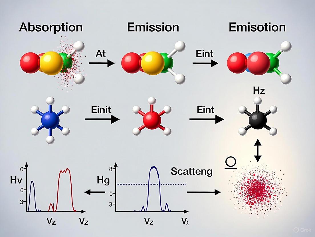
Diagram 1: Absorption spectroscopy process and electron transitions

Complementary Nature of Absorption and Emission Spectra

Absorption and emission spectra represent complementary manifestations of the same quantum mechanical transitions between energy states. The absorption spectrum appears as dark lines superimposed on a continuous spectrum, corresponding precisely to the bright lines observed in the emission spectrum of the same element [13]. This inverse relationship occurs because:

• Absorption lines correspond to photon energies that match energy differences between electronic states
• Emission lines correspond to photons released when electrons transition from higher to lower energy states
• The specific wavelengths absorbed or emitted are identical for a given element, as both processes involve the same energy level differences [13]

Table 2: Comparative Analysis of Spectroscopic Processes

Process	Energy Transfer	Spectral Characteristics	Key Applications
Absorption	Photon energy transferred to molecule	Discrete lines at specific wavelengths	Chemical identification, concentration measurement
Emission	Molecular energy released as photon	Discrete lines at specific wavelengths	Elemental analysis, astronomical spectroscopy
Rayleigh Scattering	No net energy transfer	Continuous spectrum, same frequency as source	Atmospheric phenomena, structural analysis
Raman Scattering	Energy exchange with molecule	Frequency-shifted lines	Molecular vibration studies, structural analysis

Experimental Methodologies

Photoelectron Spectroscopy (PES)

Photoelectron spectroscopy represents a direct application of the photoelectric effect for investigating electronic structures of atoms, molecules, and solids. PES quantitatively measures kinetic energies of photoelectrons ejected by photon irradiation, enabling determination of binding energies, intensities, and angular distributions of these electrons [15].

The technique divides into two primary categories based on ionization energy sources:

• X-ray Photoelectron Spectroscopy (XPS): Utilizes high-energy X-rays (1000-1500 eV) to eject electrons from core atomic orbitals, providing information about elemental composition and chemical states [15]
• Ultraviolet Photoelectron Spectroscopy (UPS): Employs ultraviolet radiation (<41 eV) to eject electrons from valence orbitals, revealing details about molecular orbital energy levels [15]

The fundamental equation governing PES derives from the photoelectric effect: [Ek = h\nu - EB] where (Ek) represents the measured photoelectron kinetic energy, (h\nu) denotes the known photon energy, and (EB) indicates the electron binding energy [15].

The phenomenological three-step model describes photoemission from solids:

• Photoabsorption: Photon absorption causes direct optical transition between occupied and unoccupied electronic states [11]
• Travel to Surface: Excited electron propagates toward material surface, potentially scattering with other constituents [11]
• Escape into Vacuum: Electron transmits through surface barrier into vacuum for detection [11]

Absorption Spectroscopy Techniques

Absorption spectroscopy methodologies measure the attenuation of electromagnetic radiation as it passes through a sample material. The basic experimental arrangement involves directing a generated radiation beam through a sample and detecting transmitted intensity [14].

Key measurement considerations include:

• Reference Spectra: Measuring radiation spectrum without sample establishes baseline characteristics [14]
• Sample Spectra: Remeasuring with sample in place identifies absorption features [14]
• Spectral Combination: Comparing reference and sample spectra yields material-specific absorption spectrum [14]

The Beer-Lambert law provides quantitative relationship between absorption and concentration: [A = \varepsilon l c] where (A) represents absorbance, (\varepsilon) denotes molar absorptivity, (l) indicates path length, and (c) signifies concentration [14].

Table 3: Absorption Spectroscopy Techniques Across Electromagnetic Spectrum

Technique	Radiation Type	Energy Transition	Typical Applications
X-ray Absorption Spectroscopy	X-rays	Inner shell electrons	Elemental analysis, material characterization
UV-Vis Absorption Spectroscopy	Ultraviolet-Visible	Valence electrons	Concentration measurement, chemical kinetics
IR Absorption Spectroscopy	Infrared	Molecular vibrations	Functional group identification, compound verification
Microwave Absorption Spectroscopy	Microwave	Molecular rotations	Molecular structure determination

Advanced Spectroscopic Applications

Contemporary research employs sophisticated spectroscopic techniques to investigate complex molecular interactions:

Vibrational Stark Effect: This method utilizes vibrational probes (typically nitriles) to measure electric fields within molecular environments. The nitrile vibrational frequency shifts linearly with applied electric field in aprotic environments, enabling quantification of electrostatic contributions to non-covalent interactions [16]. This approach has been implemented within metal-organic frameworks (MOFs) to systematically build and characterize non-covalent interactions with precise geometrical control [16].

Infrared Spectroscopy with DFT Calculations: Combining experimental IR spectroscopy with density functional theory (DFT) computations enables detailed investigation of molecule-surface interactions. This methodology has revealed pronounced vibrational blue shifts, such as CO adsorption on UO₂(111) surfaces shifting from 2143 cm⁻¹ (gas phase) to 2160 cm⁻¹, providing insights into surface chemical bonding and relativistic effects [17].

Research Reagents and Materials

Table 4: Essential Research Reagents and Materials for Spectroscopic Experiments

Reagent/Material	Function	Application Example
Monochromatic Light Source	Provides precise wavelength photons	Determining threshold frequencies in photoelectric effect
Metal Electrodes (e.g., Cs, K, Ca)	Low work function surfaces	Enhancing photoelectron emission efficiency
Vacuum Systems	Eliminates electron-gas molecule collisions	Photoelectron spectroscopy measurements
Nitrile Vibrational Probes	Electric field sensing via Stark effect	Quantifying non-covalent interactions in MOFs
Reference Compounds	Spectral calibration and quantification	Beer-Lambert law concentration determinations
Metal-Organic Frameworks (MOFs)	Precise molecular scaffolding	Systematic study of non-covalent interactions
UV-Transparent Containers	Sample housing for spectroscopy	Absorption measurements in ultraviolet region

Applications in Scientific Research

Pharmaceutical and Biomedical Applications

Spectroscopic techniques provide critical analytical capabilities throughout drug development pipelines:

• Metabolite Screening: Analyzing metabolic profiles and pathways for pharmaceutical compounds [18]
• Protein Characterization: Determining protein structure, folding, and interaction dynamics [18]
• Drug Structure Optimization: Guiding molecular design through precise measurement of chemical properties [10]

Magnetic Resonance Spectroscopy (MRS), often coupled with MRI technology, enables non-invasive diagnosis and monitoring of chemical changes in tissues, facilitating detection of conditions ranging from depression to tumors through metabolic profiling [18].

Environmental and Astronomical Spectroscopy

Absorption spectroscopy enables remote sensing applications with particular significance for environmental monitoring and astronomical investigation:

• Pollutant Identification: Infrared gas analyzers distinguish atmospheric pollutants from expected constituents through characteristic absorption signatures [14]
• Greenhouse Effect Studies: Analyzing atmospheric absorption of infrared radiation reveals mechanisms underlying global warming [13]
• Exoplanet Characterization: Measuring absorption spectra during planetary transits determines atmospheric composition, temperature, pressure, and mass of extrasolar planets [14]

Astronomical spectroscopy leverages the Doppler effect (redshift/blueshift) in spectral lines to determine celestial object velocities relative to Earth, enabling measurements of galactic motion and universe expansion [13].

Diagram 2: Relationship between fundamental processes and applications

The photoelectric effect and electron transitions constitute the fundamental physical mechanisms underlying absorption spectroscopy and related analytical techniques. The quantized nature of energy transfers between matter and electromagnetic radiation enables precise determination of molecular composition, structure, and dynamics across scientific disciplines. Contemporary research continues to refine spectroscopic methodologies, enhancing sensitivity and expanding applications from single-molecule investigations to astronomical observations. The integration of theoretical frameworks with experimental innovation ensures spectroscopy remains an indispensable tool for scientific advancement, particularly in pharmaceutical development where molecular-level understanding drives therapeutic progress.

Following the absorption of energy, an atom in an excited state must return to a lower energy state through processes collectively known as atomic relaxation. A critical pathway for this energy release is fluorescence, which involves the emission of a photon. The probability that an excited atom will de-excite through this radiative pathway, rather than a non-radiative one, is quantified by its fluorescence yield [4] [19]. This parameter is fundamental across spectroscopic techniques, from X-Ray Fluorescence (XRF) to Atomic Fluorescence Spectrometry (AFS), as it directly influences the intensity of the measured signal and the ultimate sensitivity of an analytical method [20] [19]. Understanding these mechanisms is therefore essential for optimizing spectroscopic instrumentation and interpreting experimental data, particularly in research and drug development where precise elemental detection is crucial.

Fundamental Atomic Relaxation Mechanisms

When an inner-shell electron is ejected, typically by an incident X-ray photon, the atom is left in a highly unstable, excited state. The subsequent return to stability involves a cascade of possible electronic transitions, which can be categorized into radiative and non-radiative processes.

The following diagram illustrates the core atomic relaxation pathways that compete to de-excite an atom following the initial ionization event.

Radiative Relaxation: Fluorescence

Fluorescence is a radiative process where the energy released during an electron transitioning from a higher to a lower energy state is emitted as a photon [4] [19]. The emitted photon, known as characteristic X-ray radiation, has an energy specific to the element and the electronic orbitals involved, forming the basis for elemental identification in techniques like XRF [20].

Non-Radiative Relaxation: The Auger Effect

In the Auger effect, the energy from an electron filling an inner-shell vacancy is transferred to another electron within the same atom (e.g., from the L-shell), which is then ejected as a Auger electron [20]. This is a non-radiative process that competes directly with fluorescence emission. The kinetic energy of the ejected Auger electron is characteristic of the element.

Quantitative Parameters: Fluorescence Yield and Transition Probabilities

The relaxation process is governed by well-defined atomic parameters. The key quantitative factors that determine the probability and nature of the emitted radiation are summarized below.

Table 1: Key Atomic Parameters Governing X-ray Fluorescence Intensity [20]

Parameter	Symbol	Description	Impact on Fluorescence
Fluorescence Yield	ωK	Probability of radiative (vs. Auger) relaxation after a core-hole creation.	Directly proportional; higher yield means stronger signal.
Absorption Jump Ratio	JK	Ratio of mass absorption coefficients across an absorption edge; probability that a photoelectric interaction ejects a K-shell electron.	Determines the fraction of absorbed photons that create a specific core-hole.
Transition Probability	gKα	Relative probability that a specific transition (e.g., Kα) occurs among all possible transitions from a given shell.	Determines the intensity distribution of spectral lines (e.g., Kα vs Kβ).

The overall probability for producing a specific fluorescent line, known as the excitation factor (Q), is the product of these individual probabilities [20]: Q = (Absorption Jump Ratio) × (Transition Probability) × (Fluorescence Yield)

The fluorescence yield varies significantly across the periodic table, as shown in the table below.

Table 2: Experimentally Determined K-Shell Fluorescence Yields (ω_K) and Transition Probabilities (g_Kα) for Selected Elements [20]

Element	Atomic Number	K-Shell Fluorescence Yield (ωK)	Kα / Kβ Intensity Ratio	Kα Transition Probability (gKα)
Fe (Iron)	26	0.347	6.78	0.882
Cu (Copper)	29	0.440	7.65	0.884
Mo (Molybdenum)	42	0.765	5.39	0.843
W (Tungsten)	74	0.958	-	-

Experimental Methodology in Atomic Fluorescence Spectrometry

Atomic Fluorescence Spectrometry (AFS) leverages the principles of fluorescence yield for ultra-trace elemental analysis. The following diagram outlines the core workflow for an AFS experiment.

Core Experimental Protocols

Sample Atomization and Vapor Generation

• Objective: Convert the elemental analyte in a liquid or solid sample into a cloud of free, gaseous atoms in the instrument's observation zone (atom cell) [19].
• Protocol for Hydride-Forming Elements (As, Se, Hg, Sb):
  • Liquid Sample Introduction: An acidified liquid sample is introduced into a vapor generation system.
  • Chemical Reduction: For elements like As and Se, a reducing agent (e.g., sodium tetrahydroborate, NaBH₄) is added to convert the element into a volatile hydride (e.g., AsH₃, H₂Se) [19].
  • Mercury Cold Vapor: Mercury is reduced to elemental mercury vapor directly.
  • Gas-Liquid Separation: The generated gaseous hydrides or vapor are separated from the liquid matrix and transported by an inert gas (e.g., Argon) into the atom cell.
• Alternative Atom Cells: Electrothermal atomizers (graphite furnaces) or inductively coupled plasmas (ICP) can also be used to produce ground-state atoms from a wider range of elements [19].

• Objective: Selectively excite the analyte atoms and detect the resulting fluorescence photons.
• Excitation Protocol:
  • A high-intensity, tuned light source (e.g., a hollow cathode lamp or tunable laser) is directed at the atom cloud [19].
  • The wavelength of the source is set to match a strong absorption line of the analyte element, promoting ground-state atoms to an excited electronic state via stimulated absorption [19].
• Detection Protocol:
  • The resulting fluorescence is collected at a direction (often 90°) to the excitation beam to minimize scattered background radiation.
  • For non-resonance fluorescence, the detected wavelength is different from the excitation wavelength, further reducing scatter [19].
  • A wavelength-selective detector (monochromator or polychromator with photomultiplier tube or CCD) measures the intensity of the specific fluorescence line.
  • The signal intensity is proportional to the concentration of the analyte in the original sample.

The Scientist's Toolkit: Essential Research Reagents and Materials

Table 3: Key Reagents and Materials for Atomic Fluorescence Spectrometry [19]

Item	Function / Description
Sodium Tetrahydroborate (NaBH4)	A strong reducing agent used to generate volatile hydrides from elements like As, Se, and Sb for introduction into the atom cell.
High-Purity Acids (HNO3, HCl)	Used for sample digestion, preservation, and acidification to enable the vapor generation reaction.
Tunable Laser Systems	High-radiance excitation sources that can saturate the atomic transition, maximizing the excited state population and fluorescence signal.
Electrothermal Atomizer (Graphite Furnace)	An electrically heated graphite tube that thermally decomposes a liquid sample to produce a cloud of free atoms.
Hydride Generation System	A specialized accessory consisting of a gas-liquid separator and pumps to generate and introduce analyte hydrides into the atom cell.
Hollow Cathode Lamps (HCLs)	Line sources that emit light characteristic of a specific element, used for selective excitation in AFS.

Advanced Considerations and Analytical Figures of Merit

Sensitivity and Quantum Yield

The sensitivity in AFS is directly dependent on the excitation source intensity, as it increases the population of the excited state. However, this relationship holds true until the system reaches saturation, where the rates of stimulated absorption and stimulated emission equalize [19]. In practical atom reservoirs like atmospheric-pressure flames, collisions with other molecules can deactivate excited states without photon emission, a process known as quenching. The fraction of atoms that emit a fluorescence photon after absorption is the quantum yield (Φ), which can be very low in high-collision environments but close to 1 in low-pressure cells [19].

Calibration and Interferences

At low concentrations, fluorescence intensity is linear with analyte concentration. However, at elevated concentrations, self-absorption can occur, where emitted fluorescence photons are re-absorbed by other atoms of the same element in the ground state within the atom cell. This leads to curvature in the calibration graph and, in extreme cases, can cause the calibration curve to roll over [19]. For hydride-generation AFS, it is critical to note that different species of an element (e.g., methylated vs. inorganic Arsenic) can form hydrides at different rates and efficiencies, potentially requiring species-specific calibration [19].

Fluorescence yield is a fundamental atomic property that dictates the efficiency of the radiative relaxation pathway. Its precise understanding, coupled with the detailed mechanisms of competing processes like the Auger effect, forms the theoretical foundation for powerful analytical techniques like XRF and AFS. By optimizing experimental parameters such as excitation source intensity and atomization conditions, and by accounting for factors like quantum yield and self-absorption, researchers can leverage these principles to achieve exceptional analytical sensitivity. This enables applications ranging from the quality control of metal alloys to the detection of trace elements and species in biological and environmental matrices, providing invaluable data for scientific research and drug development.

In spectroscopy research, the interaction of light with matter is foundational. While absorption and emission processes involve the direct exchange of energy between photons and a material, scattering describes processes where light is deflected from its original path, often undergoing changes in direction, polarization, or energy in the process [21]. Understanding the distinct mechanisms of Rayleigh, Raman, and Mie scattering is crucial for interpreting spectroscopic data, designing experiments, and developing analytical applications across scientific disciplines, including drug development. These phenomena are not merely sources of noise or loss; they are powerful probes of molecular structure, particle size, and material composition. This guide provides an in-depth examination of these core scattering processes, framed within the broader context of how light interacts with matter in spectroscopic research.

Theoretical Foundations of Light Scattering

Fundamental Definitions and Processes

Light scattering encompasses a range of phenomena governed by the interaction between an incident electromagnetic wave and the electrons within a molecule or particle. The fundamental process can be conceptualized as the oscillating electric field of a photon inducing a polarization in the molecular electron cloud [22] [23]. This transiently forms a higher-energy "virtual state," from which a photon is almost immediately re-emitted as scattered light [23]. Scattering processes are broadly categorized as either elastic or inelastic. In elastic scattering, the energy (and thus wavelength) of the scattered photon is unchanged from the incident photon. In inelastic scattering, energy is exchanged between the photon and the molecule, resulting in a shift in the wavelength of the scattered light [21]. The following table summarizes the core characteristics of the primary scattering types.

Table 1: Fundamental Types of Light Scattering

Scattering Type	Energy Change	Particle Size (relative to λ)	Key Characteristic	Typical Application
Rayleigh	Elastic (No change)	Much smaller than λ [24]	~λ⁻⁴ wavelength dependence [21]	Determining molecular polarizability [22]
Raman	Inelastic (Change in ν)	Much smaller than λ	Molecular "fingerprint" spectra [23]	Chemical identification and structure
Mie	Elastic (No change)	Similar to or larger than λ [25]	Strong forward scattering [21] [26]	Particle sizing, cloud physics

The Interaction Cross-Section

A critical quantitative parameter in scattering theory is the scattering cross-section, denoted as σs. It represents the effective area that a particle presents to the incident radiation for scattering and has units of area (e.g., m² or cm²). The cross-section quantifies the probability that a scattering event will occur. For Rayleigh scattering by a gas, the cross-section can be calculated using the refractive index and the King correction factor [27]: $$σν = \frac{24π^3ν^4}{N^2} \left( \frac{nν^2-1}{nν^2+2} \right)^2 Fk(ν)$$ where (ν) is the wavenumber, (N) is the gas number density, (nν) is the refractive index, and (Fk(ν)) is the King correction factor accounting for molecular non-sphericity [27]. Accurate knowledge of these cross-sections is essential for applications ranging from atmospheric radiative transfer models to the calibration of high-finesse optical cavities used in trace gas detection [27].

Rayleigh Scattering

Physical Mechanism and Theory

Rayleigh scattering is the elastic scattering of light by particles much smaller than the wavelength of the radiation [21] [24]. The physical mechanism involves the electric field of the incident light inducing an oscillating electric dipole in the molecules or small particles [24] [22]. This oscillating dipole then radiates light at the same frequency in all directions, acting as the source of the scattered light. Because the process is coherent and elastic, the inner energy of the scattering particles remains unchanged [21]. The intensity of Rayleigh-scattered light has an extreme dependence on the wavelength of light, scaling with the inverse fourth power of the wavelength (~λ⁻⁴) [21] [24]. This means that shorter wavelength blue light is scattered much more efficiently than longer wavelength red light.

Key Applications and Experimental Manifestations

The most familiar manifestation of Rayleigh scattering is the blue color of the daytime sky [24]. As sunlight passes through the atmosphere, its blue component is scattered far more strongly by oxygen and nitrogen molecules than other colors, giving the sky its characteristic hue. Conversely, at sunrise and sunset, sunlight travels through a thicker layer of atmosphere, scattering away most of the blue light and leaving the direct light from the sun appearing reddish [24]. In optical technology, Rayleigh scattering is the dominant source of propagation loss in high-quality optical glass fibers at shorter wavelengths (e.g., in the visible and ultraviolet ranges) [21]. This scattering occurs at microscopic, unavoidable density fluctuations in the glass. Consequently, the lowest propagation losses in silica fibers are achieved at longer, infrared wavelengths around 1.5-1.6 μm [21]. Rayleigh scattering is also routinely used to create image contrast in microscopy and in display screens [21].

Quantitative Measurement in Gases

Advanced spectroscopic techniques like Broadband Cavity-Enhanced Spectroscopy (BBCES) are used for precise, direct measurement of Rayleigh scattering cross-sections in gases. The following table details key reagents and materials used in such experiments.

Table 2: Research Reagent Solutions for Rayleigh Scattering Cross-Section Measurement

Reagent/Material	Function in Experiment
Calibration Gases (He, N₂)	Used to calibrate the path length of the optical cavity; their well-known cross-sections provide a reference [27].
Sample Gases (CO₂, N₂O, SF₆, O₂, CH₄)	Gases whose Rayleigh scattering and absorption cross-sections are being measured [27].
High-Finesse Optical Cavity	Two high-reflectivity mirrors between which light is reflected thousands of times, creating a very long effective path length for sensitive extinction measurement [27].
Broadband Light Source	A laser-driven light source (e.g., Xenon arc lamp) that provides light across a continuous wavelength range (e.g., 307–725 nm) [27].
High-Resolution Spectrometer	Analyzes the intensity of light transmitted through the optical cavity as a function of wavelength [27].

The experimental protocol involves filling the BBCES cavity with a sample gas at a specific pressure. The decay rate of light intensity (or its reciprocal, the ring-down time) within the cavity is measured with and without the sample gas. The difference in these decay rates is directly related to the extinction coefficient of the gas, from which the scattering cross-section is derived [27]. The workflow for this measurement is outlined in the diagram below.

Raman Scattering

Physical Mechanism and Theory

Raman scattering is an inelastic scattering process where there is an exchange of energy between the incident photon and the scattering molecule [28] [23]. This results in the scattered photon having a different energy, and therefore a different wavelength, than the incident photon. The process is mediated by a short-lived virtual state and involves a change in the molecular polarizability during vibration [23]. There are two types of Raman scattering:

• Stokes Raman scattering: The molecule gains energy, and the scattered photon has a lower energy (longer wavelength) than the incident photon.
• Anti-Stokes Raman scattering: The molecule loses energy, and the scattered photon has a higher energy (shorter wavelength) than the incident photon [28] [23].

At thermal equilibrium, the majority of molecules reside in the ground vibrational state, making Stokes scattering statistically more probable and thus more intense than anti-Stokes scattering [23]. The energy difference between the incident and scattered light is called the Raman shift, and it corresponds directly to the vibrational energy levels of the molecule, providing a unique spectroscopic "fingerprint" [23].

Instrumentation and Selection Rules

Modern Raman spectroscopy almost exclusively uses lasers as excitation sources due to their high intensity and monochromaticity, which is necessary to observe the weak Raman effect [28]. The scattered light is typically detected with high-sensitivity charge-coupled devices (CCDs) [28]. The selection rule for a vibration to be Raman active is that the molecular polarizability must change during the vibration ((∂α/∂Q ≠ 0)) [28]. This is in contrast to infrared (IR) absorption spectroscopy, which requires a change in the permanent dipole moment. This difference in selection rules makes Raman and IR spectroscopy complementary techniques; some vibrational modes may be active in one but not the other. For a non-linear molecule with N atoms, the number of fundamental vibrational modes is 3N-6, any of which can be Raman-active [23].

Advanced Application: Determining the Standard Chemical Potential

Raman scattering, particularly when combined with advanced techniques like femtosecond two-dimensional (2D) spectroscopy, can be used to probe fundamental thermodynamic properties of materials. For quantum-confined systems like PbS quantum dots, which have inherent structural heterogeneity, ensemble absorption and emission spectra are broadened by static inhomogeneities. 2D spectroscopy can separate this static inhomogeneity from the dynamic linewidth. By applying single-molecule generalized Einstein relations to the dynamical absorption and emission spectra obtained from 2D fits, researchers can determine the standard chemical potential difference ((Δμ^o_{j,0→X})) between the lowest excited and ground electronic states [29]. This potential defines the maximum photovoltage the excited state can generate, a critical parameter for energy applications. Furthermore, the ensemble Stokes' shift, in conjunction with these relations, can be used to determine the average single-molecule dynamical linewidth [29].

Mie Scattering

Physical Mechanism and Theory

Mie scattering describes the elastic scattering of light by spherical particles whose diameter is comparable to or larger than the wavelength of the incident light [25] [26]. Unlike Rayleigh scattering, which can be treated as a simple oscillating dipole, the Mie solution requires solving Maxwell's electromagnetic equations for the interaction of a plane wave with a homogeneous sphere, taking into account phase variations and contributions from multiple electric and magnetic multipoles [25] [30]. The full Mie solution is expressed as an infinite series of spherical multipole partial waves [25]. Key features that distinguish Mie scattering from Rayleigh scattering include:

• A much weaker dependence on wavelength.
• A pronounced asymmetry in angular distribution, with a strong preference for forward scattering [21] [26].
• The appearance of Mie resonances, where the scattering efficiency oscillates as a function of the size parameter (x = 2πr/λ) [26].

Applications and Observational Evidence

Mie scattering is responsible for the white appearance of clouds [21] [25]. The water droplets in clouds have sizes on the order of the wavelength of visible light, and all wavelengths are scattered approximately equally, resulting in the white or gray color we observe. This is in stark contrast to the blue sky caused by Rayleigh scattering. Mie theory is essential in a wide range of fields, including meteorological optics, biomedical optics (e.g., light scattering by cells), and for characterizing colloidal suspensions and aerosols [21] [26]. It is the theoretical foundation for laser diffraction particle sizing instruments, which inversely calculate particle size distributions from measured scattering patterns [26]. The following diagram illustrates the core logic of Mie theory and its application to particle characterization.

Table 3: Key Characteristics of Mie Scattering for Different Particle Sizes

Particle Size Regime	Wavelength Dependence	Angular Distribution	Scattering Efficiency (σ/πa²)
Rayleigh (x << 1)	Strong (~λ⁻⁴)	Symmetric (forward = backward)	Proportional to (a/λ)⁴ [26]
Mie Resonance (x ≈ 1)	Oscillatory and complex	Multiple maxima/minima, stronger forward lobe	Oscillates with size parameter [26]
Large Particle (x >> 1)	Nearly independent of λ	Very strong forward lobe, diffraction pattern	Approaches 2 (extinction paradox) [26]

Comparative Analysis and Research Implications

Integrated Framework for Spectroscopy Research

In practical spectroscopy research, Rayleigh, Raman, and Mie scattering phenomena are not isolated events but represent different facets of light-matter interaction that must be considered holistically when designing and interpreting experiments. The choice of excitation wavelength in a spectroscopic application is often a compromise between these processes. For instance, in fluorescence spectroscopy, a common technique in drug development, Rayleigh scattering can overlap with and obscure weak emission signals, while Raman scattering from the solvent can create interfering peaks. Selecting a longer excitation wavelength can reduce Rayleigh scattering (due to its λ⁻⁴ dependence) and minimize this interference, but it must be balanced against the absorption profile of the fluorophore. Similarly, the development of sensors based on elastic (Rayleigh or Mie) scattering must account for the particle size of the analyte and the resulting wavelength dependence and angular distribution of the scattered signal [22].

Technological and Methodological Synergies

The distinctions between scattering mechanisms are leveraged in advanced instrumentation. Broadband Cavity-Enhanced Spectroscopy (BBCES), as described for Rayleigh cross-section measurement, fundamentally relies on the wavelength-dependent nature of the scattering loss within the cavity to determine gas concentrations and properties [27]. Confocal Raman microscopy spatially filters light to suppress out-of-focus Rayleigh and Mie scattered light, allowing for the clear detection of the weaker inelastically Raman-scattered photons used for chemical identification. Furthermore, the combination of scattering techniques with absorption and emission measurements, as demonstrated by 2D spectroscopy, provides a more complete picture of a material's electronic and vibrational structure, enabling the determination of key parameters like the standard chemical potential of excited states [29]. Understanding these core scattering phenomena is therefore not merely an academic exercise but a practical necessity for pushing the boundaries of analytical science, materials characterization, and pharmaceutical development.

Spectroscopy and spectrometry are foundational techniques in analytical science, yet the terms are often used interchangeably, leading to conceptual ambiguity. For researchers and drug development professionals, a precise understanding of the distinction is crucial for both methodological design and data interpretation. Spectroscopy constitutes the theoretical science investigating the interactions between radiated energy and matter [18] [31]. It is the study of how matter absorbs, emits, or scatters electromagnetic radiation to reveal information about its structure and dynamics [4]. In contrast, spectrometry represents the practical application used to acquire quantitative measurements of a spectrum [18] [32]. It is the methodological process of generating and measuring spectral data, often using instruments called spectrometers [33].

This distinction frames a critical partnership: spectroscopy provides the theoretical models for understanding energy-matter interactions, while spectrometry supplies the empirical data that validates and refines those models. Within drug development, this synergy enables everything from elucidating molecular structures to quantifying analyte concentrations in complex biological matrices.

Core Principles: Absorption, Emission, and Scattering

The theoretical framework of spectroscopy is built upon three fundamental molecular processes: absorption, emission, and scattering. These interactions between molecules and electromagnetic radiation reveal crucial information about molecular energy states, composition, and dynamics [4].

Absorption and Emission Processes

Absorption occurs when a molecule takes in energy from incident electromagnetic radiation, causing a transition from a lower energy state to a higher, excited state. The probability of absorption is determined by the transition dipole moment, which depends on the change in the molecule's electronic, vibrational, or rotational state [4].

Emission is the reverse process, where an excited molecule releases energy as electromagnetic radiation when returning to a lower energy state. This occurs through two primary mechanisms:

• Spontaneous emission: An excited molecule spontaneously decays to a lower energy state, emitting a photon with energy corresponding to the difference between states.
• Stimulated emission: An incident photon interacts with an excited molecule, inducing the emission of a second photon with identical energy, phase, and direction [4].

The intensity of absorbed or emitted radiation depends on the population of molecules in the initial and final energy states, governed by the Boltzmann distribution [4].

Scattering Phenomena

Scattering redirects electromagnetic radiation without net energy transfer to the molecule. Several scattering processes provide distinct spectroscopic information:

• Rayleigh scattering: An elastic process where radiation interacts with a molecule and is re-emitted at the same frequency. The intensity of Rayleigh scattering is proportional to the square of the molecular polarizability and inversely proportional to the fourth power of the radiation wavelength [4].
• Raman scattering: An inelastic process where the scattered radiation frequency shifts due to transitions between vibrational or rotational energy states. Stokes Raman scattering occurs at lower frequency (higher wavelength) when molecules transition to higher energy states, while Anti-Stokes Raman scattering occurs at higher frequency (lower wavelength) when molecules transition from higher to lower states [4].
• Brillouin scattering: An inelastic process involving interaction with acoustic phonons (collective vibrational modes) in materials, resulting in small frequency shifts determined by acoustic phonon velocity and incident radiation wavelength [4].

Table 1: Characteristics of Molecular Spectroscopy Processes

Process	Energy Transfer	Spectral Characteristics	Key Applications
Absorption	Molecule gains energy	Discrete peaks at specific wavelengths	Quantitative analysis, concentration determination [14]
Emission	Molecule releases energy	Discrete peaks at specific wavelengths	Elemental analysis, fluorescence spectroscopy
Rayleigh Scattering	No net transfer	Same frequency as incident radiation	Atmospheric science, particle size analysis [4]
Raman Scattering	No net transfer	Frequency-shifted peaks	Molecular fingerprinting, bond vibration analysis [4]

Spectroscopic and Spectrometric Techniques: A Comparative Analysis

The principles of absorption, emission, and scattering form the basis for diverse analytical techniques. The distinction between spectroscopy (theoretical framework) and spectrometry (measurement application) manifests across multiple methodological domains.

Major Spectroscopic Techniques

Absorption Spectroscopy encompasses techniques that measure radiation absorption as a function of frequency or wavelength [14]. The absorption spectrum reveals electronic, vibrational, and rotational energy level structures. Major subtypes include:

• Ultraviolet-Visible (UV-Vis) Spectroscopy: Measures electronic transitions in molecules; widely used for concentration determination via the Beer-Lambert law [32].
• Infrared (IR) Absorption Spectroscopy: Probes vibrational transitions in molecular bonds; essential for functional group identification and molecular fingerprinting [18].
• X-ray Absorption Spectroscopy: Investigates inner-shell electron excitations; provides information about atomic environment and oxidation states [14].

Emission Techniques include:

• Optical Emission Spectroscopy (OES): Excites atoms to higher energy states, then analyzes characteristic wavelengths emitted as they return to ground states; extensively used for elemental analysis in metallurgy [31].
• Atomic Emission Spectroscopy: Similar to OES but specifically focuses on atomic rather than molecular emissions.

Scattering-Based Techniques include:

• Raman Spectroscopy: Exploits inelastic scattering to provide vibrational fingerprints complementary to IR spectroscopy [4].
• Brillouin Spectroscopy: Measures frequency shifts from acoustic phonon interactions; used to determine elastic properties of materials [4].

Spectrometric Implementation

Spectrometry implements spectroscopic theory to generate quantitative measurements. Key spectrometric methods include:

• Mass Spectrometry (MS): Measures mass-to-charge ratio of ions; identifies molecular weights and structures [18] [31].
• Ion-Mobility Spectrometry (IMS): Separates ions based on size, shape, and charge in a carrier gas under an electric field [31].
• Rutherford Backscattering Spectrometry (RBS): Analyzes backscattered ions from a sample to determine composition and layer thickness [31].

Table 2: Spectroscopy vs. Spectrometry Comparative Analysis

Aspect	Spectroscopy	Spectrometry
Primary Focus	Theoretical study of energy-matter interactions [18] [31]	Quantitative measurement of spectral data [18] [32]
Nature	Conceptual framework	Practical application and measurement
Output	Understanding of interaction mechanisms	Numerical data, spectra, quantifiable results [33]
Key Question	How does matter interact with radiation?	What is the intensity at specific wavelengths/mass-to-charge ratios?
Example Techniques	Absorption theory, Emission theory, Scattering theory	Mass spectrometry, Ion-mobility spectrometry [31]

Experimental Protocols and Methodologies

Protocol for Absorption Spectroscopy Measurements

Principle: Determine the presence and concentration of a substance by measuring its absorption of electromagnetic radiation at characteristic wavelengths [14].

Materials and Equipment:

• Light source (e.g., deuterium lamp for UV, tungsten lamp for visible)
• Monochromator or wavelength selector
• Sample holder (cuvette with defined path length)
• Photodetector
• Data acquisition system

Procedure:

• Instrument Calibration: Power on the spectrophotometer and allow it to warm up for 15-30 minutes. Calibrate using a blank/reference sample containing only the solvent [33].
• Sample Preparation: Prepare analyte solutions at appropriate concentrations. For solid samples, ensure proper mounting to minimize light scattering.
• Baseline Correction: Measure the blank solution to establish a baseline, accounting for solvent absorption and reflection losses.
• Spectral Acquisition: Introduce the sample and measure absorbance across the desired wavelength range (e.g., 200-800 nm for UV-Vis).
• Quantitative Analysis: Apply the Beer-Lambert law (A = εlc, where A is absorbance, ε is molar absorptivity, l is path length, and c is concentration) to determine unknown concentrations [14].

Data Interpretation: Absorption peaks indicate electronic or vibrational transitions characteristic of specific functional groups or molecular structures. Peak intensity correlates with concentration, while peak position provides structural information.

Protocol for Mass Spectrometric Analysis

Principle: Identify and quantify compounds by measuring mass-to-charge ratios of gas-phase ions [18].

Materials and Equipment:

• Ionization source (e.g., electron impact, electrospray ionization)
• Mass analyzer (e.g., quadrupole, time-of-flight, orbitrap)
• Ion detector (e.g., electron multiplier)
• High vacuum system
• Data processing software

Procedure:

• Sample Introduction: Introduce the sample via direct probe, liquid chromatography, or gas chromatography interface.
• Ionization: Convert sample molecules to gas-phase ions using an appropriate ionization technique (e.g., ESI for biomolecules, EI for small molecules).
• Mass Analysis: Separate ions based on mass-to-charge ratio (m/z) using electric and/or magnetic fields.
• Detection: Measure abundance of separated ions at the detector.
• Data Analysis: Interpret the mass spectrum to identify compounds based on molecular ions, fragment patterns, and accurate mass measurements.

Applications in Drug Development: MS is indispensable for metabolite identification, pharmacokinetic studies, protein characterization, and quality control of pharmaceutical compounds [18].

Visualizing Spectroscopic and Spectrometric Relationships

The following diagrams illustrate the conceptual relationship between spectroscopy and spectrometry, along with the fundamental processes underlying spectroscopic analysis.

Diagram 1: Theoretical-practical relationship in spectral analysis.

Diagram 2: Fundamental processes in molecular spectroscopy.

The Scientist's Toolkit: Essential Research Reagents and Materials

Successful spectroscopic analysis requires appropriate selection of reagents, reference materials, and instrumentation components. The following table details essential items for a comprehensive spectroscopy laboratory.

Table 3: Essential Research Reagents and Materials for Spectroscopic Analysis

Item	Function	Application Examples
Reference Standards	Calibration and quantification	Certified elemental standards for OES, pharmaceutical reference standards for UV-Vis assay development [14]
Solvents (HPLC/UV-Vis Grade)	Sample preparation and dilution	Methanol, acetonitrile, and water for preparing samples for UV-Vis, IR, or MS analysis [33]
Cuvettes/Sample Cells	Sample containment for measurement	Quartz cuvettes for UV-Vis, NaCl plates for IR spectroscopy, NMR tubes [33]
Matrix Compounds	Sample preparation for MSI	Matrix-assisted laser desorption/ionization (MALDI) matrices like α-cyano-4-hydroxycinnamic acid for MS imaging [34]
Deuterated Solvents	NMR spectroscopy	Deuterated chloroform (CDCl₃), dimethyl sulfoxide (DMSO-d₆) for NMR solvent suppression
Ionization Reagents	Facilitating ion formation in MS	Trifluoroacetic acid (TFA) for ESI-MS, electron impact ionization gases for GC-MS
Calibration Mixtures	Instrument performance verification	Polystyrene standards for molecular weight determination, wavelength calibration standards [33]

Emerging Trends: AI and Advanced Data Analysis in Spectroscopy

The integration of artificial intelligence (AI) and chemometrics represents a paradigm shift in spectroscopic analysis. While classical methods like principal component analysis (PCA) and partial least squares (PLS) regression remain vital, they are now complemented by advanced AI frameworks that automate feature extraction, nonlinear calibration, and data fusion [35].

Machine Learning Applications:

• Supervised Learning: Algorithms including Support Vector Machines (SVMs) and Random Forests are trained on labeled spectral data to perform regression or classification tasks, enabling automated spectral quantification and compositional analysis [35].
• Unsupervised Learning: Techniques like PCA and clustering discover latent structures in unlabeled spectral data, valuable for exploratory analysis and outlier detection [35].
• Deep Learning: Convolutional Neural Networks (CNNs) and other deep neural architectures automatically extract hierarchical features from raw spectral data, particularly effective for processing unstructured data sources like hyperspectral images [35].

In pharmaceutical applications, AI-enhanced spectroscopy enables rapid, non-destructive analysis for drug authentication, quality control, and biomedical diagnostics. These approaches improve classification accuracy and feature selection while providing interpretable insights into spectral-chemical relationships [35].

The distinction between spectroscopy as a theoretical framework and spectrometry as practical measurement remains fundamental to analytical science. Spectroscopy provides the conceptual models for understanding absorption, emission, and scattering processes, while spectrometry delivers the quantitative measurements that validate these models and extract chemically relevant information. For drug development professionals, this synergy enables sophisticated molecular characterization, quantitative analysis, and structural elucidation essential to modern pharmaceutical research. As spectroscopic technologies continue to evolve, particularly with the integration of artificial intelligence and advanced data analysis methods, this foundational partnership between theory and measurement will continue to drive innovation in analytical methodology.

Element selectivity is a foundational principle of modern X-ray spectroscopy, allowing researchers to probe the specific chemical state and local environment of a chosen element within complex, multi-component materials. This capability is primarily enabled by the existence of unique, element-specific absorption edges—sharp increases in X-ray absorption that occur when the incident photon energy matches the binding energy of a core-level electron. This technical guide details the fundamental mechanisms of absorption edges, their critical role in advanced analytical techniques like X-ray Absorption Near Edge Structure (XANES) and Extended X-ray Absorption Fine Structure (EXAFS), and their application through contemporary, AI-enhanced workflows in fields ranging from battery research to pharmaceutical development.

In the realm of materials characterization, the ability to interrogate a specific element without interference from the surrounding matrix is a powerful analytical advantage. Element selectivity is this very capability, and in X-ray spectroscopy, it is achieved through the exploitation of absorption edges [36]. An absorption edge is a sharp discontinuity in the absorption spectrum of a substance that occurs at a wavelength where the energy of an incident photon corresponds precisely to the binding energy of a specific core-level electron (e.g., 1s, 2p) in a particular element [37]. When the photon energy surpasses this threshold, a photoelectron is ejected, resulting in a significant increase in the absorption probability.

This phenomenon is the cornerstone of techniques like X-ray Absorption Spectroscopy (XAS). Because the binding energies of core electrons are unique to each element, tuning the incident X-ray energy to a specific absorption edge allows researchers to selectively excite and study one element at a time, even in complex systems such as catalysts, battery electrodes, or biological tissues [36] [38]. The absorption edge not only identifies the element but also serves as a reference point for detailed analysis of its local electronic and structural environment.

Fundamental Physics of Absorption Edges

The physical process underlying the absorption edge is the photoelectric effect. An incident X-ray photon is absorbed by an atom, and its energy is transferred to a core electron. If the photon energy is sufficient to overcome the electron's binding energy, the electron is ejected from its core shell into an unoccupied state or the continuum, leaving behind a core hole [39]. The sudden increase in absorption coefficient at this specific energy is the absorption edge.

The naming convention for absorption edges is based on the principal quantum number of the shell from which the electron is ejected. The most common edges used in spectroscopy are:

• K-edge: Corresponds to the excitation of a 1s electron.
• L-edge: Corresponds to the excitation of a 2s or 2p electron. Due to spin-orbit splitting, the L-edge is often subdivided into L1 (2s), L2 (2p₁/₂), and L3 (2p₃/₂) edges [40] [39].
• M-edge and beyond: Correspond to excitations from shells with principal quantum number 3 and higher.

Table 1: Standard X-ray Absorption Edge Nomenclature

Edge Name	Electron Shell	Sub-levels
K-edge	1s	---
L-edge	2s, 2p	L1 (2s), L2 (2p₁/₂), L3 (2p₃/₂)
M-edge	3s, 3p, 3d	M1 (3s), M2 (3p₁/₂), M3 (3p₃/₂), M4 (3d₃/₂), M5 (3d₅/₂)
N-edge	4s, 4p, 4d, 4f	...

The Photoelectric Effect and Absorption Process

The following diagram illustrates the fundamental process that gives rise to an absorption edge.

Diagram 1: Photoelectric Effect at the Absorption Edge. An incident X-ray photon is absorbed by an atom, ejecting a core electron and creating a core hole.

The absorption coefficient (μ) of a material is not a smooth function of energy. As demonstrated in the diagram, when the energy of the incident radiation (E) scans through the binding energy regime of a core shell, a sudden, sharp increase in absorption appears—this is the absorption edge [39]. The exact energy of an element's absorption edge is a fingerprint, allowing for its unambiguous identification.

Element-Selective Techniques: XANES and EXAFS

The absorption edge itself is just the starting point for analysis. The fine structure in the absorption spectrum around the edge provides rich, quantitative information. This fine structure is divided into two primary regions, which form the basis of two powerful, element-selective techniques.

X-ray Absorption Near Edge Structure (XANES)

The X-ray Absorption Near Edge Structure (XANES) region encompasses the spectrum from just below the absorption edge to approximately 30-50 eV above it [40] [38]. This region is exquisitely sensitive to the oxidation state and local coordination geometry of the absorbing atom.

• Oxidation State: A shift in the absorption edge position to higher energies indicates an increase in the oxidation state of the element. This is because a higher positive charge on the nucleus increases the binding energy of the core electrons, requiring more energy to eject them [38].
• Coordination Chemistry: The shape and presence of pre-edge peaks (weak transitions below the main edge) and the "white line" (the first strong peak after the edge) provide information about the symmetry of the local environment (e.g., octahedral vs. tetrahedral coordination) and the density of unoccupied electronic states [41] [39].

Extended X-ray Absorption Fine Structure (EXAFS)

Beyond the XANES region, extending to about 1000 eV above the edge, the Extended X-ray Absorption Fine Structure (EXAFS) manifests as oscillatory variations in the absorption coefficient [40] [42]. These oscillations result from the interference between the outgoing photoelectron wave and the waves backscattered from neighboring atoms. Analysis of EXAFS provides quantitative data on:

• Interatomic distances (bond lengths)
• Coordination numbers
• Identity of neighboring atoms
• Structural disorder (thermal and static) [40] [42]

Table 2: Comparative Analysis of XANES and EXAFS

Feature	XANES (X-ray Absorption Near Edge Structure)	EXAFS (Extended X-ray Absorption Fine Structure)
Spectral Region	~ -10 eV to +30-50 eV from edge	~ 50 eV to 1000 eV above edge
Primary Information	Oxidation state, coordination chemistry, electronic structure (density of unoccupied states)	Local atomic structure: coordination numbers, bond lengths, identity of neighbors, disorder
Underlying Physics	Electronic transitions to unoccupied bound states; multiple scattering resonances	Single and multiple scattering of the photoelectron from neighboring atoms
Data Interpretation	Often used as a "fingerprint" for qualitative comparison; quantitative analysis requires theoretical calculations.	Quantitative fitting using theoretical standards to extract structural parameters.

Advanced Experimental Methodologies

Translating the theoretical principles of absorption spectroscopy into reliable data requires robust experimental protocols.

Data Collection Modes

The absorption coefficient can be measured in several ways, each suited to different sample types [36]:

• Transmission Mode: Measures the intensity of the X-ray beam before (I₀) and after (Iₜ) it passes through the sample. It is the most direct method and is ideal for homogeneous samples where the element of interest is a major component (e.g., concentrated powder pellets).
• Fluorescence Mode: Measures the intensity of the characteristic fluorescent X-rays (I_f) emitted as the atom relaxes from its core-hole state. This mode is essential for dilute systems or thin films where the element of interest is present in low concentrations, as it offers a higher signal-to-noise ratio.
• Electron Yield Mode: Measures the current of electrons (Auger and secondary electrons) emitted during the relaxation process. This method is highly surface-sensitive.

Protocol: Multi-Edge EXAFS with Reverse Monte Carlo (RMC) Analysis

For complex materials, such as bimetallic oxides, single-edge analysis can be insufficient. The following protocol, as applied to SrTiO₃, details a sophisticated approach for resolving three-dimensional local structures, including light atoms like oxygen [42].

• Sample Preparation: Mix the powder sample (e.g., SrTiO₃) with a boron nitride binder and press into a homogeneous pellet.
• Data Collection: Collect EXAFS spectra in transmission mode at multiple absorption edges (e.g., Sr-K and Ti-K edges) across a temperature range of interest.
• Data Pre-processing: Use software like ATHENA for background subtraction, normalization, and Fourier transformation of the raw absorption data.
• Reverse Monte Carlo (RMC) Simulation:
  • Model Setup: Create an initial supercell atomic cluster (e.g., 6x6x6 unit cells) based on known crystallographic data.
  • Path Calculation: Use a code like FEFF to calculate hundreds of photoelectron scattering paths for each absorption edge, including multiple scattering effects.
  • Iterative Fitting: The RMC algorithm (e.g., within the EvAX code) randomly adjusts atomic positions in the cluster. After each move, it calculates the theoretical EXAFS spectra for both edges simultaneously and compares them to the experimental data using a goodness-of-fit parameter.
  • Convergence: The process runs for tens of thousands of steps until the fit converges, resulting in a three-dimensional atomic configuration that is consistent with all experimental EXAFS spectra.

This two-metal-edge RMC method provides a stereoscopic view of the local structure, allowing for the precise measurement of bond angles and the detection of subtle phenomena like oxygen octahedral rotations, which are often missed in single-edge analysis [42].

Protocol: AI-Driven Adaptive Sampling for Dynamic XANES

Traditional XANES data collection can be time-consuming. For dynamic processes (e.g., battery cycling), an AI-driven adaptive sampling method can drastically reduce data collection time while preserving critical information [41].

• Initial Sparse Sampling: Collect a small set of initial measurement points across the energy range of interest (e.g., 10-20% of a conventional dense grid).
• Gaussian Process (GP) Modeling: Use the acquired data to build a GP model. This model provides a posterior mean (the predicted spectrum) and a posterior standard deviation (the uncertainty) at every unmeasured energy point.
• Acquisition Function Calculation: Calculate an acquisition function (e.g., maximizing uncertainty reduction) across the energy range to identify the most informative next measurement point.
• Iterative Loop: Measure the point suggested by the acquisition function, update the GP model with the new data, and recalculate the acquisition function to select the next point. This loop continues until a pre-defined accuracy threshold is met.
• Spectrum Reconstruction: The final set of sparse measurements is used to reconstruct the full XANES spectrum.

This knowledge-injected Bayesian optimization approach has been shown to accurately reconstruct XANES spectra using only 15–20% of the typical measurement points, enabling higher time resolution for tracking rapid chemical changes [41].

The Scientist's Toolkit: Essential Research Reagents and Materials

The following table catalogues key resources and tools used in modern XAS experiments.

Table 3: Essential Tools and Resources for X-ray Absorption Spectroscopy

Item / Resource	Function & Explanation
Synchrotron Radiation Source	Provides the intense, tunable, and monochromatic X-ray beam required to scan across absorption edges. Essential for high-quality XAS data.
Double Crystal Monochromator	An energy-adjustable device that selects a specific X-ray energy from the broad synchrotron spectrum with high precision [41].
Ionization Chambers	Detectors used in transmission mode to measure the intensity of the X-ray beam before (I₀) and after (Iₜ) it passes through the sample [36].
Fluorescence Detector	A dedicated detector (e.g., a multi-element solid-state detector) used in fluorescence mode to measure the intensity of emitted X-rays from the sample.
Reference Materials	Standard samples of known structure and chemical state (e.g., metal foils) used for energy calibration and as benchmarks for data analysis [43].
FEFF Code	A widely used software for ab initio calculations of XAS spectra. It generates theoretical scattering paths used for EXAFS fitting and XANES interpretation [44].
ATHENA Software	A popular graphical software package for standard XAS data processing, including alignment, background subtraction, normalization, and Fourier transformation [36].
XAS Databases (e.g., XASDB, XASLIB)	Public databases of experimental and theoretical XAS spectra that allow researchers to compare their data with known references, aiding in material identification and interpretation [43].

AI and Data Science in Modern XAS Analysis

The field of XAS is being transformed by artificial intelligence and machine learning (ML), which are helping to bridge the gap between theoretical simulation and experimental data.

• Spectral Domain Mapping (SDM): A key challenge is that ML models are often trained on perfect simulated data but are applied to noisy experimental data. SDM is a data-driven approach that transforms experimental spectra into a simulation-like representation, improving the reliability of ML predictions on real-world data [44].
• Universal ML Models: Research is advancing towards developing foundation models trained on XAS data across the entire periodic table. These models can leverage common trends across different elements, enhancing their predictive power and generalizability [44].
• Database-Driven Discovery: The creation of large, curated databases of experimental XAS spectra, such as XASDB, provides the essential data infrastructure for training and validating these advanced AI models, fostering a new era of data-driven scientific discovery [43] [44].

Absorption edges are a critical physical phenomenon that unlock the power of element-selective analysis in X-ray spectroscopy. By providing a unique entry point to probe specific elements, techniques like XANES and EXAFS offer unparalleled insights into oxidation states, local coordination, and atomic-scale structure. The continued evolution of these methods—through advanced protocols like multi-edge RMC analysis, AI-accelerated data collection, and the growing ecosystem of computational tools and databases—ensures that absorption edge spectroscopy will remain a cornerstone technique for addressing the most complex challenges in materials science, chemistry, and drug development.

Analytical Techniques and Pharmaceutical Applications: From API Characterization to Biologics

X-ray Absorption Spectroscopy (XAS) is a powerful analytical technique used for probing the local electronic and geometric structure around a specific element in a material. As a photon-in/photon-out spectroscopy, it provides element-specific information, making it invaluable for studying complex systems in chemistry, materials science, and biology [45] [46]. The technique's unique capability to analyze amorphous solids, liquid systems, and heterogeneous samples without requiring long-range order has established it as a versatile structural probe complementary to diffraction methods [45] [47].

Within the broader context of a thesis on absorption, emission, and scattering in spectroscopy, XAS represents a fundamental process where matter absorbs X-ray photons, leading to electronic excitations. The subsequent relaxation processes, which may involve fluorescence emission or non-radiant Auger decay, form the basis for related techniques like X-ray Emission Spectroscopy (XES), creating a comprehensive spectroscopic toolkit for investigating material properties [48]. This technical guide examines the core principles, methodologies, and applications of XAS, with particular emphasis on its growing importance in pharmaceutical research where it enables the study of drug-metal interactions, speciation of elements in biological systems, and characterization of active pharmaceutical ingredients (APIs) [49] [36].

Fundamental Principles of XAS

Core Concepts and Physical Basis

XAS is founded on the photoelectric effect, where an incident X-ray photon is absorbed by an atom, exciting a core electron to either an unoccupied bound state or ejecting it into the continuum as a photoelectron [50] [36]. This process creates a core hole in the inner electronic shell, with the absorption probability increasing sharply when the incident photon energy matches the binding energy of a core-level electron, producing a characteristic "absorption edge" [36]. The element-specific nature of these edges enables targeted investigation of selected elements by tuning the excitation energy to their characteristic absorption edges [36].

The experimental measurement involves recording the absorption coefficient (μ) as a function of incident photon energy, typically by measuring the attenuation of the X-ray beam through a sample (transmission mode) or by detecting secondary processes like fluorescence emission that result from the absorption event [36]. The resulting spectrum is conventionally divided into two main regions: the X-ray Absorption Near-Edge Structure (XANES) and the Extended X-ray Absorption Fine Structure (EXAFS) [45] [47].

Table 1: Fundamental Transitions and Corresponding Absorption Edges in XAS

Principal Quantum Number (n)	Shell Notation	Electron Excitation	Edge Name
1	K	1s	K-edge
2	L	2s, 2p	L-edge
3	M	3s, 3p, 3d	M-edge

The information content differs significantly between the XANES and EXAFS regions of the spectrum. XANES provides insights into electronic structure, including oxidation state, coordination chemistry, and site symmetry through bound-state electronic transitions and multiple-scattering resonances [51] [47]. In contrast, EXAFS arises from single-scattering events of the ejected photoelectron with neighboring atoms, providing quantitative information about interatomic distances, coordination numbers, and neighbor identities [45] [47].

Figure 1: Fundamental Processes in X-ray Absorption Spectroscopy

Theoretical Framework

The theoretical foundation of XAS involves understanding the wave behavior of the photoelectron ejected during the absorption process. The wave vector (k) of the photoelectron, which determines the specific subset of XAS techniques applicable for analysis, can be derived from the photoelectron's kinetic energy [50]:

The kinetic energy (Eₖ) of the photoelectron is given by:

[Ek = E - E0]

where E is the incident X-ray energy and E₀ is the threshold energy required to promote the electron into the continuum. The wave vector k is then expressed as:

[k = \sqrt{\left(\frac{2\pi}{h}\right)^2 2m(h\nu - E_0)}]

where h is Planck's constant, m is the electron mass, and hν is the incident photon energy [50]. The different regimes of k determine whether XANES or EXAFS analysis is appropriate, with XANES corresponding to lower k-values (typically k < 2/Å) where multiple scattering dominates, and EXAFS corresponding to higher k-values where single scattering events prevail [50].

The distinction between XANES and EXAFS regions, while conventionally set at approximately 50 eV above the absorption edge, is fundamentally based on these scattering differences [51]. In the XANES region, the photoelectron has low kinetic energy and undergoes multiple scattering events with surrounding atoms, making this region particularly sensitive to electronic structure and three-dimensional geometry [51]. In the EXAFS region, the photoelectron has higher kinetic energy and typically undergoes single scattering events, providing more straightforward information about interatomic distances and coordination numbers [45].

XAS Methodology and Experimental Framework

Experimental Setup and Measurement Modes

Modern XAS experiments predominantly utilize synchrotron radiation sources due to their high photon flux, broad tunable energy range, and excellent stability characteristics [47]. These properties are essential for obtaining high signal-to-noise data within reasonable time frames, particularly when studying elements at low concentrations or conducting time-resolved experiments [47]. A typical XAS experiment requires several key components: a monochromator for energy selection (commonly using silicon crystals with (111), (220), or (400) orientations), ionization chambers for incident intensity measurement, and appropriate detectors for measuring transmitted or emitted signals [47].

Table 2: Comparison of XAS Measurement Modes

Measurement Mode	Detection Method	Sample Requirements	Advantages	Limitations
Transmission	Measures intensity after passing through sample (Iₜ) relative to incident beam (I₀)	Homogeneous samples with element concentration >10%; uniform thickness [36]	High-quality spectra with short acquisition time [36]	Requires specific sample characteristics; not suitable for dilute systems
Fluorescence	Measures characteristic X-ray emission (I_f) using dedicated detectors	Dilute systems, low concentrations, heterogeneous samples [36] [47]	High sensitivity for trace elements; reduced background	Self-absorption effects can distort spectra [36]
Electron Yield	Measures electrons emitted due to absorption processes	Surface-sensitive studies; conducting samples	Surface sensitivity (~nm depth)	Limited to conductive samples or thin layers; vacuum typically required

The experimental arrangement varies depending on the measurement mode. In transmission geometry, ionization chambers are placed before and after the sample to directly measure beam attenuation [47]. For fluorescence measurements, the detector is typically placed at 90 degrees to the incident beam, with both the beam and detector at 45 degrees relative to the sample surface normal to minimize background scattering [36]. The choice of measurement strategy depends on the sample characteristics and the specific scientific questions being addressed, with each approach offering distinct advantages and limitations.

The Scientist's Toolkit: Essential Research Reagents and Materials

Table 3: Essential Materials and Equipment for XAS Experiments

Item	Function/Purpose	Technical Considerations
Synchrotron Beamline	Provides intense, tunable X-ray source	Essential for high-flux requirements; enables rapid measurements (minutes per spectrum) [45] [47]
Crystal Monochromator	Selects specific X-ray energy from broad spectrum	Common crystals: Si(111), Si(220), Si(400); choice affects energy resolution and flux [45] [47]
Ionization Chambers	Measures incident (I₀) and transmitted (Iₜ) beam intensities	Filled with appropriate gas mixtures (e.g., N₂, Ar) for optimal detection efficiency [47]
Fluorescence Detector	Measures characteristic X-ray emission	Solid-state detectors (e.g., Ge, Si) with high energy resolution; arranged at 90° geometry [36]
Sample Holder	Contains and positions sample during measurement	Material depends on X-ray energy (e.g., Kapton, Teflon, aluminum); must not absorb strongly at energies of interest
Reference Standard	Energy calibration and instrument validation	Metallic foils (e.g., Cu, Fe) for edge energy calibration; measured simultaneously with sample

Figure 2: Experimental Setup for X-ray Absorption Spectroscopy

Data Interpretation and Analysis

XANES: Probing Electronic Structure and Oxidation States

XANES (X-ray Absorption Near-Edge Structure) encompasses the spectral region from a few eV below the absorption edge to approximately 50 eV above it [51] [47]. This region is dominated by multiple scattering resonances and transitions to quasi-bound states, making it highly sensitive to the electronic structure and three-dimensional geometry around the absorbing atom [45] [51]. The most prominent feature in a XANES spectrum is the absorption edge itself, which corresponds to the transition to the lowest unoccupied states [45].

The precise energy position of the absorption edge provides crucial information about the oxidation state of the absorbing atom. For metals, the edge shifts to higher energies with increasing oxidation state due to the enhanced core-electron binding energy resulting from decreased shielding in more highly charged ions [51] [52]. This relationship enables quantitative determination of oxidation states through comparison with appropriate reference compounds of known oxidation states [52].

The pre-edge region, occurring at energies slightly below the main absorption edge, contains valuable information about electronic transitions to bound states. For transition metals, pre-edge features often correspond to transitions to molecular orbitals with significant d-character [45] [51]. The intensity and energy distribution of these pre-edge features provide insights into coordination geometry, site symmetry, and covalent bonding effects [51]. For instance, the intensity of pre-edge features in octahedrally coordinated transition metal compounds is typically enhanced in centrosymmetric complexes due to mixing of p- and d-orbitals [51].

EXAFS: Determining Local Atomic Structure

EXAFS (Extended X-ray Absorption Fine Structure) extends from approximately 50 eV to 1000 eV above the absorption edge and arises from the interference between the outgoing photoelectron wave and the portion backscattered from neighboring atoms [45] [47]. The EXAFS signal, typically denoted as χ(k), is extracted from the raw absorption spectrum through a multi-step process involving background subtraction, normalization, and conversion from energy to photoelectron wave vector space [47].

The EXAFS equation provides the theoretical foundation for quantitative analysis:

[ \chi(k) = \sumj \frac{Nj S0^2 Fj(k)}{k Rj^2} \sin(2kRj + \phij(k)) e^{-2\sigmaj^2 k^2} e^{-2R_j/\lambda(k)} ]

where:

• Nⱼ is the number of atoms in the jth shell
• Rⱼ is the distance to the jth shell
• Fⱼ(k) is the backscattering amplitude
• φⱼ(k) is the phase shift
• σⱼ² is the Debye-Waller factor representing disorder
• λ(k) is the photoelectron mean free path
• S₀² is the amplitude reduction factor [47]

Fourier transformation of the EXAFS signal χ(k) yields a radial distribution function that provides a visual representation of the atomic environment around the absorbing atom, with peaks corresponding to coordination shells at approximately 0.3-0.5 Å less than the actual bond distances due to the phase shift φⱼ(k) [47]. Quantitative structural parameters, including interatomic distances (with precision of ~0.01-0.02 Å), coordination numbers (accurate to 10-20%), and disorder parameters, can be extracted through nonlinear least-squares fitting of theoretical models to experimental data [47].

Advanced Applications in Pharmaceutical Sciences

Drug Development and Biopharmaceutical Applications

While XAS has found broad application across numerous scientific disciplines, its implementation in pharmaceutical research, though still emerging, has demonstrated significant potential [36]. The technique's element selectivity enables targeted investigation of specific metal centers in metallodrugs and metalloproteins without interference from the complex biological matrix [49] [36]. This capability is particularly valuable for studying the local atomic structure and oxidation states of metal-containing active pharmaceutical ingredients (APIs), which is crucial for understanding their mechanism of action, stability, and bioavailability [49] [36].

One notable application involves studying interactions between components in parenteral nutrition solutions, particularly zinc and amino acids, which can modify their bioavailability [49]. XAS has enabled characterization of these interactions at the molecular level, providing insights that inform formulation strategies to optimize drug delivery and efficacy [49]. Similarly, EXAFS analysis of copper-amino acid complexes has supported the development of efficient oral drugs for treating copper deficiencies in Menkes disease, illustrating how structural information obtained through XAS can directly guide therapeutic development [49].

The technique has also proven valuable for characterizing novel metal-based therapeutics, such as arsenic-containing drugs for leukemia, where XANES and EXAFS analysis allowed researchers to determine the solution form of the drug, a critical factor influencing its pharmacological behavior [49]. When combined with complementary techniques like synchrotron-radiation-excited X-ray fluorescence for mapping trace elements along patient hair samples, XAS provides a comprehensive approach for monitoring essential trace elements during therapy [49].

Machine Learning and Future Directions

Recent advances in data analysis methodologies, particularly the integration of machine learning (ML) approaches, are expanding the capabilities of XAS for pharmaceutical applications. Supervised ML models, such as random forest algorithms, have demonstrated remarkable success in predicting oxidation states from XAS spectra, achieving high accuracy (R² score of 0.85 for copper L-edge spectra) and enabling rapid analysis of complex mixed-valence systems [52]. These computational approaches address significant limitations of traditional analysis methods, which often rely on matching unknown spectra to experimental standards—a process requiring significant domain expertise and susceptible to experimental variations [52].

The application of ML to XAS data analysis facilitates real-time processing of large spectral datasets generated during in-situ experiments, opening new possibilities for high-throughput screening of pharmaceutical compounds and monitoring dynamic processes such as drug release or metabolic transformations [52]. Furthermore, these computational approaches enhance the ability to extract quantitative information from complex systems containing multiple oxidation states or coordination environments, a common challenge in pharmaceutical research where metal-containing drugs often exist in multiple speciation states under physiological conditions [36] [52].

As synchrotron facilities continue to develop brighter sources and more efficient detection systems, coupled with advances in computational methods, XAS is poised to become an increasingly powerful tool for pharmaceutical research. The ability to conduct operando studies of drug delivery systems, characterize metal-biomolecule interactions in physiological environments, and monitor structural changes during manufacturing processes represents just a few of the promising directions for this technique in drug development and quality control [36].

X-ray Absorption Spectroscopy stands as a versatile and powerful analytical technique that provides unique insights into the local electronic and geometric structure around specific elements in diverse materials. Its element specificity, sensitivity to local environment rather than long-range order, and applicability to various sample states (solid, liquid, gas) make it particularly valuable for pharmaceutical applications where traditional structural methods often face limitations. The complementary information provided by XANES and EXAFS—ranging from oxidation states and coordination chemistry to quantitative interatomic distances and coordination numbers—enables comprehensive characterization of metal-containing pharmaceuticals and their interactions with biological systems.

As the pharmaceutical industry continues to develop increasingly complex therapeutic agents, particularly those incorporating metal centers for catalytic or structural functions, the role of XAS in drug development is expected to expand significantly. Coupled with advances in synchrotron technology, detection methodologies, and computational analysis including machine learning, XAS offers unprecedented opportunities to elucidate structure-function relationships in pharmaceutical systems, ultimately contributing to the development of more effective and targeted therapeutics.

Molecular spectroscopy is fundamentally based on the interactions between electromagnetic radiation and matter, primarily through the processes of absorption, emission, and scattering. Absorption occurs when a molecule takes in energy from photons, transitioning from a lower to a higher energy state. Emission is the reverse process, where a molecule releases energy as photons when transitioning from a higher to a lower energy state. Scattering involves the redirection of incident radiation by a molecule, which can be either elastic (Rayleigh scattering), with no energy change, or inelastic (Raman scattering), involving energy transfer between the photon and the molecule [4]. Understanding these core processes provides the essential physical context for the measurement modalities of transmission, fluorescence, and electron yield detection discussed in this technical guide.

Core Detection Modalities: Principles and Methodologies

Transmission Detection

The transmission method is one of the most direct ways to measure X-ray absorption. It involves directing a monochromatic X-ray beam through a thin sample and measuring the intensity of the transmitted beam. The absorption coefficient (µ) is derived from the ratio of the transmitted intensity (I_t) to the incident intensity (I₀), typically expressed as µ ∝ ln(I₀/I_t) [53]. This technique requires the preparation of thin, uniform samples, such as foils or thin films, to ensure adequate transmission of the X-ray beam while providing sufficient absorption signal [53] [54]. Its implementation is relatively straightforward, but its requirement for thin samples can be a limitation for many material types.

Fluorescence Yield Detection

Fluorescence yield detection measures the intensity of characteristic X-rays emitted when an excited atom relaxes. The creation of a core hole by X-ray absorption is followed by a decay process. In the soft X-ray region, Auger decay dominates over X-ray fluorescence [53]. However, for hard X-rays, fluorescence becomes a more prominent decay channel. This method is particularly advantageous for dilute systems or thin films, as it provides a direct measure of the absorption event without the stringent sample thickness requirements of transmission measurements. The detected signal is proportional to the number of absorbed photons, making it a powerful tool for probing low concentrations of specific elements.

Electron Yield Detection

Electron yield detection measures the electrons emitted as a direct consequence of the absorption process. When an X-ray photon is absorbed, it creates a core hole. The subsequent decay of this core hole, primarily through Auger processes in the soft X-ray regime, leads to the emission of electrons [53]. The technique encompasses several distinct approaches, summarized in the table below.

Table 1: Comparison of Electron Yield Detection Techniques

Technique	Measured Signal	Sampling Depth	Key Characteristics
Total Electron Yield (TEY)	Cascade of secondary electrons [53]	Several nanometers [53]	Standard surface-sensitive measurement; simple experimental setup.
Auger Electron Yield (AEY)	Primary Auger electrons [53]	< 1 nanometer [53]	Highly surface-sensitive; requires ultra-high vacuum conditions.
Conversion Electron Yield (CEY)	Electrons ionizing surrounding gas molecules [54]	Surface-sensitive (less than penetration depth of X-rays) [54]	Can be performed under atmospheric pressure; higher signal intensity than TEY [54].

The experimental setup for CEY detection, for instance, involves placing a sample inside a chamber with an electrode designed to collect electrons that have ionized the surrounding gas molecules, preventing electron-ion recombination [54]. A key advantage of CEY is its applicability to samples with poor electrical conductivity and the reduced restrictions on sample environment compared to vacuum-based electron detection methods [54].

Comparative Analysis and Experimental Protocols

Quantitative Comparison of Detection Modalities

The choice of detection modality depends on the specific sample properties and the information required. The table below provides a structured comparison to guide this selection.

Table 2: Comparative Analysis of X-ray Absorption Detection Methods

Characteristic	Transmission	Fluorescence Yield	Total Electron Yield (TEY)	Auger Electron Yield (AEY)
Sample Requirements	Thin, uniform foils or films [53]	Bulk, thick, or dilute samples	Conventional samples [53]	Conventional samples [53]
Sampling Depth / Volume	Bulk-sensitive (entire sample thickness)	Bulk-sensitive	Surface-sensitive (~few nm) [53]	Highly surface-sensitive (<1 nm) [53]
Key Advantages	Direct measurement of absorption; quantitative [53]	Sensitive for dilute systems; reduced self-absorption effects	Universal applicability; simple setup [53]	Extreme surface sensitivity [53]
Primary Limitations	Requires optimized, thin samples [53] [54]	Lower signal in soft X-ray region [53]	Indirect absorption measurement; limited to surfaces [53]	Requires UHV; signal intensity can be low [53]

Generalized Experimental Protocol for NEXAFS Measurement

The following workflow outlines a standard procedure for collecting a NEXAFS spectrum, adaptable for the different detection modes.

Diagram 1: NEXAFS measurement workflow, showing parallel paths for different detection modes.

Procedure:

• Sample Preparation: Depending on the chosen detection mode:
  • Transmission: Prepare a thin, pinhole-free foil or film with an optimized thickness to avoid over-absorption [53].
  • TEY/AEY/CEY: Bulk samples can typically be used as-is. For CEY under atmospheric conditions, ensure the sample holder and electrode are properly configured [54].
  • Fluorescence Yield: Suitable for bulk, thick, or dilute samples.
• Sample Mounting: Secure the sample in the appropriate holder. For electron yield measurements in vacuum, ensure good electrical contact.
• Beamline Alignment: Align the monochromatic X-ray beam to illuminate the desired spot on the sample. Simultaneously, align the detectors (electron analyzer, fluorescence detector, or transmission ion chambers).
• Energy Calibration: Calibrate the monochromator energy scale using a standard sample with well-known absorption edge energies.
• Data Acquisition: Scan the monochromator energy across the absorption edge of interest. For each energy point, simultaneously record:
  • The incident photon flux (I₀).
  • The signal from the chosen detection mode(s) (I_t for transmission, electron current for TEY/AEY/CEY, or fluorescence count for fluorescence yield).
• Data Processing: Process the raw data to obtain the absorption coefficient µ(E).
  • For transmission: µ(E) ∝ ln(I₀/I_t).
  • For electron and fluorescence yield: The signal is normalized to I₀ to account for incident flux variations.

The Scientist's Toolkit: Essential Research Reagent Solutions

Table 3: Key Materials and Components for NEXAFS Experiments

Item / Reagent	Function / Application
Thin Foil Standards (e.g., Ni, Cu)	Used for energy calibration of the monochromator and for sample thickness reference in transmission mode [54].
Metal Oxide Powders (e.g., NiO)	Model systems for testing surface sensitivity and studying oxidation states, particularly in electron yield measurements [54].
Ionization Chambers	Gas-filled detectors used to measure the incident (I0) and transmitted (It) X-ray flux in transmission experiments [54].
Channeltron / Electron Multiplier	Detector for measuring low-current electron signals in Auger Electron Yield (AEY) and other electron detection schemes.
Collection Electrode (for CEY)	An electrode used in Conversion Electron Yield (CEY) to collect electrons that have ionized surrounding gas molecules, preventing recombination under atmospheric conditions [54].
Polymer & Organic Films	Standard samples for carbon K-edge NEXAFS studies, useful for demonstrating chemical sensitivity and functional group identification [53].

Advanced Applications: Probing Chemical and Magnetic Structure

The true power of these detection modalities is realized in their advanced applications, particularly when using polarized X-rays.

Chemical and Structural Analysis

NEXAFS is highly sensitive to the local bonding environment of the absorbing atom. The fine structure above an absorption edge arises from excitations into unoccupied molecular orbitals, providing a "fingerprint" for identifying chemical functional groups [53]. This is exemplified in the distinct Carbon K-edge spectra of different polymers. Furthermore, using linearly polarized X-rays, researchers can determine molecular orientation. The absorption intensity is maximized when the electric field vector of the X-rays is aligned with the direction of an empty molecular orbital. This "search-light" effect has been used, for instance, to determine that benzene molecules lie flat on a silver surface [53].

Magnetic Dichroism Studies

By employing circularly or linearly polarized light, NEXAFS can probe magnetic phenomena.

• X-ray Magnetic Circular Dichroism (XMCD): The difference in absorption between left- and right-circularly polarized light is linked to the element-specific orbital and spin magnetic moments of a ferromagnetic material [53].
• X-ray Magnetic Linear Dichroism (XMLD): The difference in absorption for different orientations of linearly polarized light relative to the magnetic axis can be used to study antiferromagnetic order [53].

The relationship between these advanced techniques and the core detection methods is illustrated below.

Diagram 2: Logical flow from core absorption and detection to advanced applications enabled by polarized X-rays.

Transmission, fluorescence, and electron yield detection represent a powerful suite of techniques for measuring X-ray absorption across diverse sample environments and information depths. The choice of modality is not merely technical but strategic, dictated by the specific scientific question—whether it requires bulk or extreme surface sensitivity, involves conductive or insulating materials, or is conducted under vacuum or ambient conditions. When integrated with the core principles of absorption and the use of polarized light, these measurement "modages" provide a comprehensive toolkit for decoding chemical identity, molecular orientation, and even magnetic structure at the molecular level.

Energy-Dispersive X-ray Spectroscopy (EDS/EDX) is a powerful analytical technique used for the elemental identification and quantification of a solid sample's chemical composition [55]. As a non-destructive method typically coupled with electron microscopy instruments like Scanning Electron Microscopes (SEM) or Transmission Electron Microscopes (TEM), EDS enables researchers to obtain valuable information about materials at macro, micro, and nanoscale levels [55] [56].

Within the broader framework of spectroscopic research, EDS operates on fundamental principles of absorption and emission. The technique involves the absorption of energy from a focused electron beam, which causes ionization of atoms in the sample, followed by the emission of characteristic X-rays as the excited atoms relax to their ground state [56] [57]. This emission spectrum serves as a unique fingerprint for elemental identification, while the intensity of emissions facilitates quantitative analysis.

Fundamental Principles

Atomic Transitions and Characteristic X-ray Generation

The physical underpinnings of EDS analysis lie in the quantum mechanical model of the atom, where electrons occupy discrete energy levels or shells bound to the nucleus [57]. When a high-energy electron beam strikes the sample, it may eject a core electron (e.g., from the K, L, or M shell) from an atom, creating an electron vacancy [56] [58]. An electron from an outer, higher-energy shell then fills this hole, and the energy difference between the two shells is released as an X-ray [58].

Each element produces X-rays at specific energy levels unique to its atomic structure, allowing identification through Moseley's Law, which establishes a direct correlation between the frequency of emitted X-rays and the atomic number [58] [59]. The nomenclature for these transitions uses the shell where ionization occurred (K, L, M) combined with Greek letters (α, β) indicating the relative intensity and origin of the transition [57].

Electron Transition Process in EDS

Spectral Interpretation

EDS data is presented as a spectrum with keV on the x-axis and peak intensity (counts) on the y-axis [59]. Elemental identification occurs when characteristic X-ray peaks are matched to known energy values for specific elements. Quantitative analysis measures the relative abundance of elements based on peak intensities, though this requires correction procedures to account for factors like X-ray absorption within the sample itself [58].

Table 1: Common Characteristic X-ray Transitions in EDS Analysis

Transition	Shell Origin	Relative Energy	Significance
Kα₁	L₃ → K	Highest intensity for K-series	Primary identification line for elements Z=11-40
Kα₂	L₂ → K	Slightly lower than Kα₁	Often overlaps with Kα₁ in EDS spectra
Kβ	M₃ → K	Higher energy than Kα	Secondary identification line
Lα	M₅ → L₃	Lower energy than K-series	Primary line for heavier elements (Z>40)
Lβ	M₄ → L₂	Higher energy than Lα	Secondary series for heavier elements

Instrumentation and Detection Systems

Core Components

Modern EDS systems integrated with electron microscopes consist of four primary components:

• Excitation Source: Typically a high-energy electron beam in SEM or TEM instruments [58]
• X-ray Detector: Most commonly a Silicon Drift Detector (SDD) that converts X-ray energy into voltage signals [56] [58]
• Pulse Processor: Measures signals from the detector and processes them for analysis [58]
• Analyzer: Computer system with specialized software for spectral display, elemental identification, and quantification [58]

Detector Technology Evolution

Early EDS systems used Si(Li) detectors requiring liquid nitrogen cooling, but most modern instruments employ Silicon Drift Detectors (SDDs) with Peltier cooling systems [58]. SDDs consist of a high-resistivity silicon chip where electrons drift toward a small collecting anode, resulting in extremely low capacitance that enables shorter processing times and very high throughput [56] [58].

SDD benefits include [58]:

• High count rates and processing capabilities
• Better energy resolution than traditional Si(Li) detectors at high count rates
• Lower dead time (time spent processing X-ray events)
• Faster analytical capabilities and more precise X-ray maps
• Ability to operate at relatively high temperatures without liquid nitrogen

Emerging technologies include superconducting microcalorimeters that combine simultaneous detection capabilities of EDS with high spectral resolution of WDS, though historically limited by low count rates and small detector areas [58].

Experimental Methodology

Sample Preparation Protocols

Proper sample preparation is critical for reliable EDS analysis:

• Sample Size and Mounting: Samples must fit within the microscope chamber and be securely mounted on appropriate stubs using conductive adhesives or tapes [58]
• Electrical Conductivity: Non-conductive samples require coating with thin layers of conductive materials (carbon, gold, or platinum) to prevent charging effects under electron beam exposure [58]
• Surface Flatness: Optimal analysis requires smooth, flat surfaces to minimize topographic effects on X-ray detection; metallurgical samples often require polishing [58]
• Representative Sampling: Ensure the analyzed region represents the material's overall composition, potentially requiring multiple analysis points [58]

Data Collection Workflow

EDS Analysis Procedure

Quantitative Analysis Procedures

Accurate quantification requires careful methodology:

• Spectrum Acquisition:

  • Accelerating voltage: Typically 2-3 times the highest characteristic X-ray energy of interest
  • Beam current: Stable, sufficient to generate adequate X-ray counts without sample damage
  • Live time: 30-100 seconds for adequate counting statistics
  • Process multiple regions for heterogeneous materials

• Elemental Identification:

  • Automatic peak identification by software
  • Manual verification to address peak overlaps (e.g., Ti Kβ and V Kα, Mn Kβ and Fe Kα)
  • Consider all possible lines for each element

• Quantitative Corrections:

  • Apply ZAF (atomic number, absorption, fluorescence) or Phi-Rho-Z corrections
  • Use standardless quantification with built-in standards or comparative analysis with certified standards
  • Account for sample geometry and detector efficiency

The Scientist's Toolkit: Essential Research Reagents and Materials

Table 2: Essential Materials and Reagents for EDS Analysis

Item	Function/Purpose	Technical Specifications
Silicon Drift Detector (SDD)	X-ray detection and energy measurement	High-resolution, Peltier-cooled, active area 40-100mm² [56] [58]
Conductive Coatings	Prevents charging on non-conductive samples	Carbon, gold, or platinum-palladium; 10-20nm thickness [58]
Certified Standard Materials	Quantitative analysis calibration	Microanalysis standards with known composition [57]
Conductive Adhesives	Sample mounting	Carbon tape, silver paint, or conductive epoxy [58]
Polishing Supplies	Surface preparation for solid samples	Alumina or diamond suspensions (0.1-1µm) [58]

Analytical Capabilities and Limitations

Elemental Range and Detection Limits

EDS can typically detect elements from boron (Z=5) to uranium (Z=92), though performance for light elements (B, C, N, O) is less efficient due to their lower X-ray yields and absorption issues [59]. Detection limits are generally in the range of 0.1-1.0 weight percent, depending on the element, sample matrix, and analysis conditions [59].

Key limitations include:

• Poor sensitivity for trace elements (concentrations <0.1%)
• Difficulty detecting low atomic number elements (Z<11) due to weak X-ray yields and absorption by detector window [59]
• Inability to detect hydrogen and helium as they lack core electrons for characteristic X-ray emission [59]
• Limited spatial resolution for bulk samples (typically 1-3 microns) due to electron beam interaction volume

Accuracy and Precision Considerations

The accuracy of quantitative EDS analysis is affected by several factors:

• Peak Overlaps: Elements with overlapping emission lines require deconvolution algorithms [58]
• Matrix Effects: X-ray absorption and fluorescence within the sample require correction models [58]
• Sample Topography: Irregular surfaces affect X-ray detection efficiency
• Standards Quality: Accuracy depends on the quality and appropriateness of reference standards

With proper calibration and correction procedures, accuracy of ±2-5% relative can be achieved for major elements, while precision is primarily limited by counting statistics.

Advanced Applications and Emerging Trends

Elemental Mapping and Live Analysis

Modern EDS systems enable elemental mapping, where the distribution of elements is visualized through color-coded maps [56]. Each pixel in the map contains full spectral information, allowing retrospective analysis of phase distributions and chemical associations [56]. Live elemental mapping technologies now allow users to scan samples in real-time to identify regions of interest before conducting detailed measurements [56].

Advanced applications include:

• HyperMap Acquisition: Complete spectral data at every pixel for post-processing [56]
• Line Scans: Compositional profiles along user-defined lines
• Chemical Phase Identification: Automated classification of phases based on compositional similarities

Complementary Techniques

EDS is often combined with other analytical methods to provide comprehensive materials characterization:

• Wavelength Dispersive Spectroscopy (WDS): Offers higher spectral resolution for separating overlapping peaks and detecting trace elements [56] [58]
• Electron Backscatter Diffraction (EBSD): Provides crystallographic information complementary to elemental data [56]
• Micro-XRF on SEM: Enables trace element detection and layer analysis [56]

Energy-Dispersive X-ray Spectroscopy remains a cornerstone technique for elemental analysis in materials characterization. Its integration with electron microscopy platforms provides unparalleled capabilities for correlating microstructural features with chemical composition. Within the framework of absorption and emission spectroscopy, EDS exemplifies how characteristic radiation emitted after electron beam excitation enables both qualitative and quantitative elemental analysis.

Ongoing developments in detector technology, particularly silicon drift detectors and superconducting microcalorimeters, continue to push the boundaries of speed, sensitivity, and resolution [58]. These advancements ensure EDS will maintain its vital role in scientific research and industrial applications across materials science, semiconductor technology, life sciences, and quality control.

Theoretical Foundation: Light-Matter Interactions

Molecular spectroscopy is fundamentally based on the interactions between electromagnetic radiation and matter, primarily through the processes of absorption, emission, and scattering. These processes reveal crucial information about molecular structure, energy states, and dynamics, forming the basis for molecular fingerprinting [4].

Absorption occurs when a molecule takes in energy from incident electromagnetic radiation, promoting it from a lower energy state to a higher energy state. The energy absorbed corresponds to specific quantized transitions—electronic, vibrational, or rotational—depending on the radiation's frequency [4] [14]. Emission is the reverse process, where a molecule in an excited state releases energy as electromagnetic radiation when returning to a lower energy state. This can occur spontaneously or be stimulated by incoming photons [4]. Scattering involves the redirection of incident radiation by a molecule. Rayleigh scattering is elastic, with no energy exchange, while Raman scattering is inelastic, involving energy transfer that provides detailed information about vibrational and rotational modes [4].

The resulting absorption spectrum provides a unique "fingerprint" of a material, as absorption lines occur at frequencies that match energy differences between quantum mechanical states of the molecules. The specificity of these spectra allows for compound identification and quantification even within complex mixtures [14].

Spectroscopy Techniques for Molecular Fingerprinting

Ultraviolet-Visible (UV-Vis) Spectroscopy

UV-Vis spectroscopy probes the electronic transitions of molecules. When molecules absorb photons in the ultraviolet (200-400 nm) or visible (400-800 nm) regions, electrons are promoted from ground states to higher energy excited states. The resulting spectra provide information on chromophores and conjugated systems, making UV-Vis invaluable for quantitative analysis of concentration through the Beer-Lambert Law [14].

Key Applications:

• Quantitative determination of analyte concentrations
• Studying conjugated organic compounds and coordination complexes
• Monitoring reaction kinetics and chemical equilibria

Infrared (IR) Absorption Spectroscopy

IR spectroscopy measures the absorption of infrared light, primarily exciting vibrational transitions in molecules. These vibrations include stretching, bending, and twisting motions of chemical bonds, with characteristic absorption frequencies that serve as highly specific molecular fingerprints. The mid-IR region (400-4000 cm⁻¹) is particularly information-rich for functional group identification and structural elucidation [14].

Key Applications:

• Identification of functional groups and molecular structures
• Quality control and raw material verification in pharmaceuticals
• Analysis of hydrogen bonding and molecular interactions

Terahertz Spectroscopy

Terahertz spectroscopy operates in the far-infrared to microwave region (0.1-10 THz), probing low-energy collective molecular motions. These include intermolecular vibrations, crystalline lattice modes, and large-amplitude torsional motions. The terahertz region provides unique fingerprints for polymorph discrimination in pharmaceutical compounds and analysis of weakly bound molecular networks [60].

Advanced Implementation: Recent breakthroughs in field-resolved spectroscopy and compressed sensing have overcome traditional limitations in terahertz fingerprinting. By implementing random scanning techniques, researchers have demonstrated precise identification of atmospheric water vapor absorption peaks up to 2.5 THz while sampling beyond the Nyquist limit, achieving a mean squared error of only 12×10⁻⁴ [60].

Comparative Analysis of Spectroscopic Techniques

Table 1: Technical Specifications and Applications of Spectroscopic Methods

Parameter	UV-Vis Spectroscopy	IR Spectroscopy	Terahertz Spectroscopy
Spectral Range	200-800 nm	400-4000 cm⁻¹ (mid-IR)	0.1-10 THz (3-333 cm⁻¹)
Primary Transitions	Electronic	Vibrational	Low-frequency vibrations, lattice modes
Information Obtained	Chromophores, conjugation, concentration	Functional groups, molecular structure	Polymorphs, collective motions, hydration
Quantitative Application	Excellent (Beer-Lambert Law)	Good	Emerging
Key Strengths	High sensitivity for quantification	Rich structural information	Penetration of materials, polymorph discrimination

Table 2: Molecular Fingerprinting Capabilities Across Spectral Regions

Aspect	UV-Vis	IR	Terahertz
Specificity	Moderate	High	Very High
Sensitivity	High (ppb for some analytes)	Moderate to High	Moderate
Sample Preparation	Minimal	Moderate to Complex	Minimal for transmission
Advanced Methods	Derivative spectroscopy, multiwavelength analysis	FTIR, ATR, 2D-IR	Time-domain spectroscopy, compressed sensing
Primary Industries	Pharmaceuticals, environmental, materials	Pharmaceuticals, polymers, chemicals	Security, pharmaceuticals, semiconductors

Advanced Methodologies and Experimental Protocols

Compressed Sensing in Terahertz Fingerprinting

Traditional spectroscopic techniques like ultrashort time-domain spectroscopy and field-resolved spectroscopy have been hampered by the Nyquist criterion, which requires sampling at least twice the highest frequency component, leading to lengthy acquisition times and substantial data volumes [60].

Experimental Breakthrough: Fattahi and colleagues demonstrated the first experimental application of compressed sensing on field-resolved molecular fingerprinting using random scanning techniques [60]. Their methodology enabled real-time field-resolved fingerprinting with greater speed and accuracy by:

• Significantly undersampling the electric field of the molecular response at a Nyquist frequency of 0.8 THz
• Precisely identifying primary absorption peaks of atmospheric water vapor up to 2.5 THz
• Achieving high accuracy with a mean squared error of 12×10⁻⁴ despite sampling beyond the Nyquist limit

This approach dramatically reduces data acquisition time and processing requirements while maintaining spectral accuracy, opening possibilities for real-time monitoring applications.

Data Processing and Visualization Protocols

Modern spectroscopic analysis relies heavily on computational tools for data processing and visualization. Python has emerged as a powerful platform for spectroscopic data analysis with libraries including:

• Matplotlib for publication-quality spectral visualization [61]
• Pandas for efficient handling of spectral DataFrames [61]
• Custom functions for data extraction, baseline correction, and multi-spectra comparison [61]

Standardized Workflow:

• Import spectral data from CSV or other standard formats
• Apply preprocessing algorithms (smoothing, baseline correction, normalization)
• Generate comparative visualizations with appropriate scaling and labeling
• Extract quantitative parameters through peak fitting and integration
• Implement statistical analysis for pattern recognition and classification

Research Reagent Solutions and Essential Materials

Table 3: Essential Tools for Spectroscopic Analysis

Item	Function	Application Notes
Reference Standards	Calibration and validation of spectral accuracy	NIST-traceable materials for quantitative work
ATR Crystals (Diamond, ZnSe, Ge)	Internal reflection element for FTIR sampling	Diamond: durable, broad range; ZnSe: general purpose; Ge: high refractive index
Spectroscopic Cells/Cuvettes	Sample containment with known pathlength	Quartz (UV-Vis), NaCl/KBr (IR), specialized windows for terahertz
Purging Gases	Remove atmospheric absorbers	Dry air or N₂ for IR; Often essential for terahertz to minimize water vapor interference
Software Packages	Spectral processing, analysis, and database search	Commercial and open-source options for peak fitting, quantification, and library searches

Signaling Pathways and Experimental Workflows

Diagram 1: Spectroscopy Experimental Workflow

Diagram 2: Photon-Matter Interaction Pathways

The optical spectroscopy toolbox provides complementary techniques for comprehensive molecular fingerprinting across multiple spectral domains. UV-Vis spectroscopy offers exceptional quantitative capabilities for electronic transitions, IR spectroscopy delivers detailed structural information through vibrational modes, and terahertz spectroscopy probes low-frequency collective motions with high specificity. The integration of advanced computational methods, including compressed sensing and Python-based data analysis, continues to expand the capabilities of these techniques. As spectroscopic technologies evolve, particularly in overcoming traditional limitations like the Nyquist criterion through innovative sampling approaches, researchers gain increasingly powerful tools for molecular analysis across pharmaceutical development, environmental monitoring, and materials characterization.

Biomedical spectroscopy leverages the interactions between light and matter to probe the molecular composition of biological systems. The core processes—absorption, emission, and scattering of electromagnetic radiation—provide a non-destructive window into cellular and sub-cellular events, enabling researchers to decipher complex biochemical profiles. Absorption occurs when a molecule takes in energy from electromagnetic radiation, causing it to transition from a lower to a higher energy state. Emission is the reverse process, where a molecule releases energy as radiation when transitioning from a higher to a lower energy state. Scattering involves the redirection of incident radiation by a molecule without a net transfer of energy, though inelastic scattering can involve energy exchange [4]. These fundamental phenomena form the basis for a suite of analytical techniques that can characterize metabolites, identify proteins, and unravel disease mechanisms with high sensitivity and specificity.

The central role of spectroscopy in systems biology is underscored by its ability to measure the functional outputs of the cellular machinery. The metabolome, in particular, offers a dynamic, comprehensive, and precise picture of the phenotype, representing the final downstream product of genomic, transcriptomic, and proteomic activity [62]. Current high-throughput spectroscopic technologies, especially mass spectrometry (MS) and nuclear magnetic resonance (NMR) spectroscopy, have allowed the discovery of relevant metabolites and proteins that characterize a wide variety of human health and disease states [62] [63]. This technical guide explores the application of these spectroscopic methods in metabolic analysis and protein characterization, detailing the underlying principles, experimental workflows, and data interpretation strategies that make them indispensable in modern biomedical research and drug development.

Metabolomics: Deciphering the Metabolic Profile

Fundamental Concepts and Biomedical Significance

Metabolomics is the comprehensive study of the metabolome, defined as the complete set of small-molecule metabolites (typically <1500 Da) within a biological system at a given point in time [64]. These metabolites—including sugars, lipids, amino acids, and nucleotides—represent the ultimate functional readout of cellular processes and provide a dynamic snapshot of the phenotype. As the field has matured, it has become a powerful tool for biomarker discovery, understanding molecular mechanisms, and advancing precision medicine [62]. The metabolome is highly sensitive to both genetic and environmental influences, reflecting factors such as disease status, drug intake, nutritional state, gut microbiota activity, and aging [64]. This sensitivity makes metabolomics particularly valuable for tracking disease progression, monitoring therapeutic interventions, and understanding complex pathophysiological processes.

Metabolomics can be broadly classified into two approaches: untargeted and targeted analysis. Untargeted metabolomics aims to detect and measure as many metabolites as possible without prior selection, providing a global overview of the metabolic state. This approach is particularly useful for hypothesis generation and discovering novel biomarkers [62]. In contrast, targeted metabolomics focuses on the precise quantification of a predefined set of metabolites, typically with higher accuracy and sensitivity. This strategy is employed for hypothesis testing and validating specific metabolic pathways [64]. The choice between these approaches depends on the research question, with each offering complementary insights into the biochemical landscape of biological systems.

Mass Spectrometry-Based Metabolomics Workflows

Mass spectrometry has emerged as a cornerstone technology for metabolomic analysis due to its high sensitivity, resolution, and ability to characterize a vast range of metabolites [64]. A typical MS-based metabolomics workflow involves multiple critical steps, each requiring careful optimization to ensure reliable and reproducible results.

The process begins with sample collection from various biological sources, including cells, tissues, blood, plasma, urine, or cerebrospinal fluid. The choice of sample matrix depends on the research question—intracellular metabolic pathways are best studied using cells or tissues, while urine may be more relevant for biomarker discovery in kidney or bladder cancers [64]. To preserve the in vivo metabolic state, rapid quenching of metabolism is essential immediately after sample collection. This is typically achieved through flash freezing in liquid nitrogen, using chilled methanol, or ice-cold PBS [64]. Following quenching, metabolite extraction is performed using organic solvents to separate metabolites from proteins and other macromolecules. Common extraction methods include liquid-liquid extraction with solvent systems like methanol/chloroform/water, which can separate polar metabolites (into the methanol/water phase) from non-polar lipids (into the chloroform phase) [64]. The specific solvent composition, pH, and extraction conditions must be optimized based on the chemical properties of the target metabolites.

For analysis, separation techniques are often coupled with MS to enhance metabolite detection. Liquid chromatography (LC), gas chromatography (GC), and capillary electrophoresis (CE) are commonly used to reduce sample complexity prior to MS analysis [62]. The mass spectrometer itself serves as the detector, measuring the mass-to-charge ratio of ionized metabolites. Key considerations in MS analysis include the choice of ionization source (e.g., electrospray ionization, ESI; or matrix-assisted laser desorption/ionization, MALDI) and mass analyzer (e.g., time-of-flight, TOF; triple quadrupole, QqQ; or Orbitrap) [64]. The resulting raw data undergoes processing including peak detection, alignment, and normalization, followed by statistical analysis to identify significant metabolic features. Finally, metabolite annotation and identification connects these features to specific chemical structures using databases such as HMDB, METLIN, and KEGG [64].

The following workflow diagram illustrates the key stages in a mass spectrometry-based metabolomics study:

Figure 1: MS-Based Metabolomics Workflow. The process begins with sample collection and proceeds through metabolic quenching, extraction, separation, mass spectrometry analysis, data processing, and final biological interpretation.

Key Research Reagents and Materials for Metabolomics

The following table details essential reagents and materials used in mass spectrometry-based metabolomics, along with their specific functions in the experimental workflow:

Table 1: Essential Research Reagents for Mass Spectrometry-Based Metabolomics

Reagent/Material	Function	Examples/Notes
Quenching Solvents	Rapidly halts metabolic activity to preserve in vivo metabolite levels	Liquid nitrogen, chilled methanol (-20°C to -80°C), ice-cold PBS [64]
Extraction Solvents	Precipitates proteins and extracts metabolites from biological matrix	Methanol/chloroform/water (classical for biphasic extraction), methyl tert-butyl ether (MTBE) for lipids [64]
Internal Standards	Corrects for technical variability and enables accurate quantification	Stable isotope-labeled metabolites (e.g., ¹³C, ¹⁵N), added at known concentrations before extraction [64]
Quality Control (QC) Pools	Monitors instrument performance and data quality throughout analysis	Pooled sample from all experimental groups, injected at regular intervals [64]
Chromatography Columns	Separates metabolites prior to MS analysis to reduce complexity	Reverse-phase (C18) for non-polar metabolites, HILIC for polar metabolites, GC columns for volatile compounds [62] [64]
Mass Calibration Standards	Ensures mass accuracy and instrument calibration	Commercially available calibration solutions specific to the mass analyzer [64]

Quality assurance and quality control (QA/QC) are critical throughout the metabolomics workflow. The Metabolomics Quality Assurance and Quality Control Consortium (mQACC) establishes best practices to ensure data reliability and reproducibility [64]. This includes using internal standards, quality control pools, and standardized protocols for sample preparation and analysis.

Targeted Proteomics in Metabolic Engineering

Principles and Applications of Targeted Proteomics

While metabolomics provides insights into the end-products of cellular processes, targeted proteomics enables precise measurement of the proteins that catalyze metabolic reactions and regulate cellular functions. This approach has become a routine tool for verifying protein expression levels and identifying bottlenecks in metabolic pathways [63]. In metabolic engineering, targeted proteomics via selected reaction monitoring (SRM) or multiple reaction monitoring (MRM) allows researchers to detect and quantify sets of proteins with high selectivity, multiplexity, and reproducibility [63]. This capability is crucial for optimizing metabolically engineered organisms, as it provides direct measurement of enzyme abundances that influence metabolic flux and product yield.

The integration of targeted proteomics with other omics technologies creates a powerful framework for understanding and manipulating cellular metabolism. When combined with genome-scale metabolic models and flux balance analysis, targeted proteomics data helps constrain and validate computational predictions of metabolic capabilities [63]. This synergistic approach has successfully boosted the production of various bio-based chemicals in metabolic engineering cell factories, from commodity chemicals to high-value pharmaceuticals [63]. By quantifying the levels of native and engineered proteins in these systems, researchers can identify rate-limiting steps in biosynthetic pathways and implement strategies to rebalance enzyme expression for improved performance.

Spectroscopic Workflow for Targeted Proteomics

Targeted proteomics employs mass spectrometry with selective monitoring of specific peptide ions, providing highly specific and sensitive protein quantification. The workflow begins with protein extraction from biological samples, followed by enzymatic digestion (typically with trypsin) to generate peptides. The resulting peptides are separated using liquid chromatography, which reduces sample complexity before mass spectrometry analysis. The core of the targeted approach lies in the MS analysis using triple quadrupole or similar instruments, where specific precursor-product ion transitions are monitored for each target protein [63]. This selective monitoring significantly enhances sensitivity and specificity compared to untargeted approaches.

The relationship between spectroscopy techniques and their applications in metabolic engineering can be visualized as follows:

Figure 2: Spectroscopy Techniques in Metabolic Analysis. Absorption, emission, and scattering processes form the foundation for analytical techniques like mass spectrometry and NMR, which enable targeted proteomics and metabolomics applications in metabolic engineering.

Experimental Protocols and Methodologies

Detailed Metabolite Extraction Protocol

The following protocol describes a standardized biphasic extraction method suitable for comprehensive metabolomic analysis of cell cultures or tissues, based on established methodologies in the field [64]:

• Sample Preparation: Rapidly harvest cells or tissue (approximately 10-20 mg) and immediately quench metabolism by submersion in liquid nitrogen. Store samples at -80°C if not processing immediately.

• Metabolite Extraction:

  • Add 400 μL of ice-cold methanol and 200 μL of ice-cold chloroform to the sample.
  • Add internal standards mixture (stable isotope-labeled metabolites) at this stage for quantification.
  • Vortex vigorously for 30 seconds and sonicate in an ice-water bath for 15 minutes.
  • Add 400 μL of ice-cold water and vortex again for 30 seconds.
  • Centrifuge at 14,000 × g for 15 minutes at 4°C to separate phases.

• Phase Separation:

  • The upper aqueous phase (methanol/water) contains polar metabolites.
  • The lower organic phase (chloroform) contains non-polar lipids.
  • Carefully transfer each phase to separate vials without disturbing the interphase.
  • Dry under nitrogen gas or using a vacuum concentrator.

• Sample Reconstitution:

  • Reconstitute the polar fraction in 100 μL of 10% methanol for hydrophilic interaction liquid chromatography (HILIC) MS analysis.
  • Reconstitute the non-polar fraction in 100 μL of 90% isopropanol/acetonitrile for reversed-phase LC-MS analysis.

• Quality Control:

  • Prepare a quality control pool by combining equal aliquots from all samples.
  • Analyze QC samples throughout the sequence to monitor instrument performance.

Targeted Proteomics Sample Preparation

For targeted proteomics analysis using selected reaction monitoring (SRM), the following protocol ensures reproducible protein quantification [63]:

• Protein Extraction and Digestion:

  • Lyse cells or tissue in appropriate buffer (e.g., RIPA buffer with protease inhibitors).
  • Quantify total protein using a standardized assay (e.g., BCA assay).
  • Reduce disulfide bonds with dithiothreitol (5 mM, 30 minutes, 56°C) and alkylate with iodoacetamide (15 mM, 30 minutes, room temperature in darkness).
  • Digest proteins with trypsin (1:20-1:50 enzyme-to-protein ratio) overnight at 37°C.
  • Stop digestion with acidification (0.5% formic acid).

• Peptide Cleanup:

  • Desalt peptides using C18 solid-phase extraction columns.
  • Dry peptides using a vacuum concentrator and reconstitute in 0.1% formic acid for LC-MS analysis.

• LC-SRM Analysis:

  • Separate peptides using nano-flow liquid chromatography with a C18 column.
  • Program the triple quadrupole mass spectrometer to monitor specific precursor-product ion transitions for each target protein.
  • Include stable isotope-labeled peptide standards for absolute quantification.

Data Analysis and Interpretation

Quantitative Spectroscopic Data in Biomedical Research

The quantitative data generated by spectroscopic techniques provides critical insights into biological systems. The following table summarizes key quantitative parameters and their significance in metabolomics and proteomics studies:

Table 2: Quantitative Data from Spectroscopic Analyses in Biomedical Research

Analytical Technique	Quantitative Parameters	Biological Significance	Typical Values/Ranges
Mass Spectrometry (Metabolomics)	Metabolite concentrations	Biomarker identification; Pathway activity	nM to mM range; Fold-changes of 1.5-10x in disease states [62]
Targeted Proteomics (SRM)	Protein abundances	Enzyme expression levels; Metabolic bottleneck identification	amol/μg to fmol/μg protein; >20% change considered biologically relevant [63]
NMR Spectroscopy	Spectral peak intensities	Metabolic profiling; Disease stratification	Relative concentrations; ppm chemical shift [62]
Absorption Spectroscopy	Absorbance units, Molar absorptivity	Biomolecule quantification; Enzyme kinetics	Beer-Lambert law: A = εlc (ε: 10³-10⁵ M⁻¹cm⁻¹) [4]
Emission Spectroscopy	Fluorescence intensity, Quantum yield	Protein folding; Molecular interactions	Quantum yield 0-1; Intensity proportional to concentration [4]

Statistical analysis is crucial for interpreting spectroscopic data. For metabolomics, both univariate (t-tests, ANOVA) and multivariate (PCA, PLS-DA) methods are employed to identify significantly altered metabolites between experimental groups [64]. For targeted proteomics, statistical significance is typically determined using replicate measurements (n≥3) with appropriate correction for multiple testing.

Integration of Multi-Omics Data

The true power of spectroscopic data emerges when metabolomic and proteomic measurements are integrated to build comprehensive models of biological systems. This integration enables researchers to connect enzyme abundance (from targeted proteomics) with metabolite levels (from metabolomics) to infer pathway activities and identify regulatory nodes [62] [63]. Such integrated analyses have revealed how transcription factors coordinate metabolic pathways in response to nutrient availability in cancer cells, and how allosteric regulators like glutathione, glutamate, and ATP modulate transcription factor activity [62]. These insights are accelerating the discovery of diagnostic markers and therapeutic targets for human diseases, particularly in metabolic disorders like obesity and diabetes, where branched-chain amino acids, acylcarnitines, and specific phospholipids show promise as biomarkers for disease severity and treatment response [62].

Biomedical spectroscopy, through the fundamental processes of absorption, emission, and scattering, provides powerful analytical capabilities for characterizing both metabolites and proteins in biological systems. Mass spectrometry-based metabolomics provides a dynamic window into the functional state of biological systems, while targeted proteomics enables precise quantification of the enzymatic machinery driving cellular processes. As these technologies continue to advance, they are increasingly being implemented in clinical settings to monitor disease progression, develop diagnostic biomarkers, and personalize therapeutic interventions [62]. Future developments will likely focus on standardizing analytical protocols, expanding metabolite databases, and improving computational tools for data integration and interpretation. The ongoing refinement of these spectroscopic applications promises to deepen our understanding of disease mechanisms and accelerate the development of novel therapeutic strategies in biomedical research and drug development.

Resonance Rayleigh scattering is a powerful elastic scattering technique that has emerged as a highly sensitive tool for analytical detection in spectroscopy research. In the broader context of light-matter interaction, RRS occupies a unique position distinct from pure absorption or emission processes. It occurs when the wavelength of incident light is at or near the molecular absorption band of the target analyte, leading to a resonance enhancement of the scattered light signal [65]. This phenomenon differs fundamentally from fluorescence emission, as RRS involves no real energy transition to excited states; instead, it relies on virtual states where electrons undergo resonance with the incident electromagnetic radiation [66].

The analytical power of RRS stems from this resonance enhancement effect, which can amplify scattering signals by several orders of magnitude compared to conventional Rayleigh scattering. When applied to metal ion detection, RRS techniques typically exploit the formation of complex structures—such as ion-association complexes or nanoparticle aggregates—that create enhanced scattering interfaces capable of producing strong, quantifiable signals even at trace concentration levels [65] [67].

Fundamental Principles and Signaling Pathways

Core Mechanism of RRS

The fundamental mechanism of RRS involves the interaction between light and matter where the scattering frequency coincides with the electron absorption frequency of the target molecule. This results in a resonance condition that dramatically enhances the scattering intensity [65]. The process can be understood through the following sequence:

• Incident Light Interaction: When light at or near the absorption wavelength of a molecule strikes the target
• Electron Resonance: The frequency of electron absorption of electromagnetic waves matches the scattering frequency
• Virtual State Formation: Electrons are promoted to virtual states (not real excited states)
• Elastic Scattering: Photons are re-emitted at the same wavelength but in different directions

This mechanism differs from photoluminescence processes as there is no real population of excited electronic states, making RRS an instantaneous scattering phenomenon rather than an absorption-emission process with a measurable lifetime [68].

RRS Signaling Pathway for Metal Ion Detection

The following diagram illustrates the signaling pathway for metal ion detection using Resonance Rayleigh Scattering:

RRS Detection Pathway - This diagram illustrates the signaling mechanism for metal ion detection via RRS, showing how complex formation leads to enhanced scattering.

Comparison of Light-Matter Interactions in Spectroscopy

Table 1: Fundamental Processes in Light-Matter Interaction Spectroscopy

Process	Energy States	Wavelength Relationship	Timescale	Key Applications
RRS	Virtual states	Same wavelength	Instantaneous (< femtoseconds)	Metal ion detection, nanoparticle sensing
Absorption	Real excited states	Different wavelength	Femtoseconds to picoseconds	UV-Vis spectroscopy, concentration measurement
Fluorescence Emission	Real excited states	Longer wavelength	Nanoseconds to microseconds	Biological imaging, immunoassays
Raman Scattering	Virtual states	Different wavelength	Instantaneous	Molecular fingerprinting, structural analysis

Experimental Methodologies and Protocols

General RRS Experimental Workflow

The following diagram outlines the core experimental workflow for RRS-based metal ion detection:

RRS Experimental Workflow - This diagram shows the key steps in conducting RRS measurements for metal ion detection.

Case Study 1: Silver Ion Detection Using Erythrosine

Experimental Protocol

Based on the study by PMC, the detection of Ag(I) using erythrosine involves the following detailed methodology [67]:

Reagents and Preparation:

• Prepare 1.0 × 10⁻³ mol/L erythrosine stock solution in distilled water
• Prepare Ag(I) standard solution (100 μg/mL) from certified reference material
• Prepare Britton-Robinson (BR) buffer solution (pH 4.4-4.6)

Procedure:

• Add 1.0 mL of BR buffer solution (pH 4.4) to a 10 mL marked test tube
• Add 1.0 mL of 2.5 × 10⁻⁴ mol/L erythrosine solution
• Add an appropriate amount of Ag(I) standard or sample solution
• Dilute to the mark with distilled water and mix thoroughly
• Allow the reaction to proceed for 5 minutes at room temperature
• Measure RRS intensity at 324 nm using a fluorescence spectrophotometer with Δλ = 0 nm

Mechanism Insight: In the weakly acidic medium (pH 4.4-4.6), the hydroxyl group of erythrosine dissociates, enabling Ag(I) to form a 1:1 electroneutral ion-association complex. This complex further aggregates into nanoparticles with an average size of approximately 45 nm due to hydrophobic interactions and van der Waals forces, significantly enhancing RRS intensity [67].

Optimization Parameters

Table 2: Optimization Conditions for Ag(I) Detection Using Erythrosine

Parameter	Optimal Condition	Effect of Deviation	Theoretical Basis
pH	4.4-4.6 (BR buffer)	Outside this range: Significant signal decrease	Hydroxy dissociation of Ery occurs specifically in this range
Erythrosine Concentration	2.5 × 10⁻⁵ mol/L	Lower: Incomplete reaction; Higher: Self-aggregation	Optimal probe-to-analyte ratio for complex formation
Reaction Time	5 min at room temperature	Shorter: Incomplete reaction; Longer: No improvement	Kinetics of ion-association and nanoparticle formation
Stability	12 hours	Longer periods: Signal degradation	Colloidal stability of formed nanoparticles
Wavelength	324 nm (maximum peak)	Other wavelengths: Reduced sensitivity	Resonance condition with absorption characteristics

Case Study 2: Mercury Ion Detection Using Gold Nanoparticles

Experimental Protocol

The methodology for Hg(II) detection using gold nanoparticle aggregation follows this protocol [69] [70]:

Reagents and Preparation:

• Synthesize ~30 nm gold nanoparticles (AuNPs) by citrate reduction method
• Prepare lysine solution (0.4 mM) as aggregation promoter
• Prepare phosphate buffer (12.5 mM, pH 7.0)

Procedure:

• Add 80 pM AuNPs to the sample solution containing Hg(II)
• Add phosphate buffer to maintain pH 7.0
• Add lysine to a final concentration of 0.4 mM
• Mix thoroughly and incubate for 10 minutes
• Measure RRS intensity at 370 nm and 550 nm
• Calculate the ratio I₆₉₀ₙₘ/I₅₅₀ₙₘ for quantitative analysis

Mechanism Insight: The detection mechanism involves the affinity of Hg(II) for gold surfaces. Initially, Hg(II) is reduced by citrate on AuNP surfaces. Lysine then promotes aggregation of Hg-covered AuNPs through its amine moieties, resulting in interparticle plasmon coupling that dramatically enhances RRS in the red region of the spectrum [69].

nanocatalysis-Based RRS for Hg(II) Detection

An alternative approach utilizes the inhibitory effect of Hg(II) on gold nanocatalysis [70]:

Procedure:

• Prepare reaction mixture containing HAuCl₄ (0.2 mM) and H₂O₂ (2.0 mM) in HCl medium (pH 1.5)
• Add AuNP nanocatalyst (5 nM) and different concentrations of Hg(II)
• Incubate at 60°C for 15 minutes
• Measure RRS intensity at 370 nm
• Observe decreased RRS signal with increasing Hg(II) concentration due to inhibition of nanocatalytic activity

Mechanism Insight: Hg(II) strongly adsorbs on AuNP surfaces to form AuNP-HgCl₄²⁻ complexes, inhibiting the electron transfer between H₂O₂ and HAuCl₄. This inhibition reduces the formation of new gold nanoparticles, resulting in decreased RRS intensity proportional to Hg(II) concentration [70].

Performance Metrics and Analytical Figures

Quantitative Performance Comparison

Table 3: Analytical Performance of RRS Methods for Metal Ion Detection

Detection System	Linear Range	Detection Limit	Selectivity	Real Sample Applications
Ag-Erythrosine [67]	0.0039-0.75 μg/mL	0.12 ng/mL	Good selectivity	Environmental water, pharmaceuticals, food
AuNP-Lysine for Hg [69]	Ratiometric (I₆₉₀/I₅₅₀)	Not specified	Good against common ions	Tap water, spring water
AuNP nanocatalysis for Hg [70]	0.008-1.33 μmol/L	0.003 μmol/L	Excellent selectivity	Water samples
General RRS Pharmaceuticals [65]	Varies by analyte	Typically ng/mL level	Variable	Antibiotics, proteins, biological molecules

Advanced RRS Techniques

HPLC Coupled with RRS Detection

The sensitivity of RRS can be combined with the separation power of HPLC for complex sample analysis [65]:

Protocol:

• Separate analytes using conventional HPLC column
• Perform post-column derivatization with RRS-active reagents
• Use zero-wavelength interval (Δλ = 0 nm) in detection
• Monitor RRS signal in real-time after separation

Applications:

• Determination of fluoroquinolones using erythrosine B
• Aminoglycosides analysis with improved sensitivity over UV detection
• Pharmaceutical compounds requiring trace-level detection

The Scientist's Toolkit: Essential Research Reagents

Table 4: Key Research Reagents for RRS-Based Metal Ion Detection

Reagent Category	Specific Examples	Function in RRS Detection	Notes & Considerations
Xanthene Dyes	Erythrosine, Phloxine, Eosin	Ion-association complex formation with metal ions	Bulky structures with positive/negative centers for electrostatic interaction
Metallic Nanoparticles	AuNPs (25-30 nm), AgNPs	Signal amplification through aggregation	Size affects scattering efficiency; stability crucial for reproducibility
Aggregation Promoters	Lysine, Arginine, Specific diamines	Facilitate nanoparticle aggregation in presence of target	Selectivity depends on molecular structure and concentration
Buffer Systems	BR buffer, Phosphate buffer, Acetate buffer	Maintain optimal pH for complex formation	pH critically affects dissociation and complex stability
Molecular Probes for SERS	Victoria Blue B, Rhodamine 6G, Safranin T	Enable complementary SERS detection	Used in dual-mode RRS-SERS approaches for verification

Resonance Rayleigh scattering represents a powerful analytical technique that leverages the fundamental principles of light scattering at resonance conditions to achieve exceptional sensitivity in metal ion detection. The methodology benefits from straightforward instrumentation, rapid analysis times, and the ability to be coupled with separation techniques like HPLC for complex sample matrices.

The future development of RRS continues to evolve with several emerging trends. The role of nanostructures in enhancing sensitivity is becoming increasingly understood, with research focusing on the precise relationship between molecular size enlargement and scattering enhancement [65]. Portable, low-cost instrumentation using LED sources and compact spectral sensors is making RRS more accessible for field-deployable applications [69]. Furthermore, the combination of RRS with complementary techniques like SERS provides orthogonal verification and expands the analytical capabilities for trace-level detection in environmental, pharmaceutical, and food safety applications.

For researchers in spectroscopy, RRS offers a valuable tool that bridges the gap between absorption and emission techniques, providing unique insights into molecular interactions and complex formation through the lens of elastic scattering phenomena.

Overcoming Analytical Challenges: Scatter Interference and Measurement Artifacts

Identifying and Correcting Scatter in UV-Vis Absorption Spectra

In ultraviolet-visible (UV-Vis) spectroscopy, the accurate measurement of sample absorbance is fundamental for quantitative analysis. However, light scattering phenomena from particulates, protein aggregates, or colloidal particles in solution can introduce significant baseline artifacts that compromise data integrity [71]. These scattering effects are frequently misinterpreted as genuine absorption, leading to inaccurate concentration calculations when applying Beer-Lambert's law. Rayleigh and Mie scattering mechanisms represent a particular challenge for researchers working with biological samples, nanomaterials, or any samples containing suspended particles [71] [72].

The interference from scattering becomes especially problematic in pharmaceutical development and drug characterization, where precise quantification of proteins, nucleic acids, or active compounds is essential. Traditional correction methods often prove inadequate when samples vary in particulate or soluble aggregate levels, necessitating more sophisticated approaches that account for the underlying physics of light scattering [71]. This technical guide examines the principles of scattering artifacts in UV-Vis spectroscopy and provides validated methodologies for their identification and correction within the broader context of absorption, emission, and scattering phenomena in spectroscopic research.

Theoretical Foundations of Light Scattering

Rayleigh and Mie Scattering Mechanisms

When light interacts with particles in a solution, several physical phenomena can occur depending on the relationship between the incident light wavelength and particle size. Rayleigh scattering predominates when particles are significantly smaller than the wavelength of incident light (typically <10% of λ), such as with soluble protein aggregates or small colloids [71] [72]. This elastic scattering process results in the redirection of light without energy transfer to the particles.

A defining characteristic of Rayleigh scattering is its wavelength dependence - the scattering intensity is inversely proportional to the fourth power of the wavelength (I ∝ λ⁻⁴) [72]. This mathematical relationship explains why scattering effects are markedly more pronounced at shorter wavelengths in the UV region and diminish toward longer wavelengths in the visible spectrum. Consequently, spectra affected by Rayleigh scattering exhibit elevated baselines that slope steeply from red to blue wavelengths, potentially obscuring genuine absorption features in the critical UV range where many biomolecules absorb strongly.

Mie scattering occurs when particle dimensions approach or exceed the wavelength of incident light, such as with large protein aggregates, precipitates, or microbial cells [71]. While less dependent on wavelength than Rayleigh scattering, Mie scattering similarly redirects light away from the detector path, resulting in measured intensity losses that conventional spectrophotometers interpret as absorption.

Distinguishing Absorption from Scattering

The fundamental distinction between true absorption and scattering lies in the fate of the photon energy. In authentic absorption, photons promote electrons to higher energy states, with the energy ultimately dissipated as heat or re-emitted as fluorescence. In scattering, photon energy remains unchanged, but the radiation direction is altered, preventing photons from reaching the detector along the expected optical path [72].

This distinction has practical implications for spectral interpretation. True absorption bands typically exhibit distinct, reproducible shapes and maxima corresponding to electronic transitions of specific chromophores. In contrast, scattering artifacts manifest as baseline offsets and sloping backgrounds without characteristic spectral features, though they can distort the line shapes of genuine absorption bands [72].

Figure 1: Light Interaction Pathways. This diagram illustrates the different mechanisms by which samples can reduce transmitted light intensity in UV-Vis spectroscopy.

Identifying Scatter in Absorption Spectra

Characteristic Spectral Signatures

Scattering artifacts exhibit distinctive spectral patterns that trained researchers can recognize. Rayleigh scattering manifests as a continuously sloping baseline that increases steadily toward shorter wavelengths according to the λ⁻⁴ relationship [72]. In severe cases, this slope can be so pronounced that it obscures absorption peaks entirely in the UV region. A telltale indicator of scattering is the apparent "absorption" in spectral regions where the analyte of interest should not absorb significantly, particularly at longer wavelengths where electronic transitions are unlikely [72].

Mie scattering typically produces less wavelength-dependent baseline elevation than Rayleigh scattering but can still cause significant distortions. The spectral signature often appears as a broad, featureless elevation across the measured wavelength range, though some wavelength dependence may still be evident. For samples with a mixture of particle sizes, both scattering mechanisms may contribute simultaneously, creating complex baseline artifacts that require sophisticated correction approaches [71].

Practical Diagnostic Approaches

A straightforward diagnostic method involves comparing spectra from serially diluted samples. In the absence of scattering, absorbance should scale linearly with concentration according to Beer-Lambert's law. With scattering artifacts, the relationship becomes nonlinear as the apparent "absorption" from scattering does not follow the same dilution factor as the genuine chromophore absorption [71].

Another practical approach involves visual inspection of the sample. While not quantitatively precise, noticeable turbidity or opalescence indicates significant scattering potential. For clear-appearing solutions that still exhibit suspicious spectral baselines, filtration through a 0.22μm or 0.45μm filter can provide diagnostic clarity - if the anomalous baseline disappears after filtration, scattering was likely the culprit [72].

Table 1: Characteristic Signs of Scattering Artifacts in UV-Vis Spectra

Scattering Type	Spectral Signature	Particle Size Range	Wavelength Dependence
Rayleigh Scattering	Steep slope increasing toward UV region	< 40 nm	Strong (∝ λ⁻⁴)
Mie Scattering	Broad elevation across spectrum	40 nm - 1 μm	Moderate to weak
Mixed Scattering	Combined sloping and elevated baseline	Multiple populations	Complex dependence

Correction Methodologies

Baseline Subtraction Approaches

Conventional baseline subtraction methods often employ single-point corrections at specific wavelengths where no analyte absorption occurs. Instrument software typically subtracts the absorbance value at this baseline wavelength (often 340 nm for UV measurements or 750 nm for visible range measurements) from all measured values across the spectrum [73]. While this approach can correct for constant baseline offsets, it fails to address the wavelength-dependent nature of scattering artifacts, particularly the steep slope characteristic of Rayleigh scattering [73].

For more effective correction of scattering artifacts, curve-fitting baseline subtraction approaches based on fundamental Rayleigh and Mie scattering equations provide superior results [71]. These methods model the actual physics of the scattering process, generating a theoretical scattering curve that is then subtracted from the measured spectrum. The parameters of the scattering equation are optimized to fit regions of the spectrum known to be free of genuine absorption, typically at longer wavelengths where the analyte does not absorb [72].

Advanced Rayleigh-Mie Correction Protocol

A validated protocol for advanced scatter correction involves multiple stages of analysis and validation [71]:

• Identification of non-absorbing spectral regions where the signal derives solely from scattering artifacts. These regions are typically at wavelengths longer than any genuine absorption features of the analyte.

• Non-linear curve fitting using scattering equations applied to the identified regions. The fundamental Rayleigh scattering equation (A = A₀ + c/λ⁴) provides the physical basis for the fit, with modifications for Mie scattering contributions when appropriate [72].

• Generation of the scattering baseline across the entire spectral range based on the fitted parameters.

• Subtraction of the calculated scattering component from the measured spectrum to yield the corrected absorption spectrum.

• Validation using control samples with known scattering properties, such as protein size standards or polystyrene nanospheres, to verify correction accuracy [71].

Table 2: Comparison of Scatter Correction Methods

Method	Principle	Advantages	Limitations
Single-Point Baseline Correction [73]	Subtracts constant offset value at specific wavelength	Simple, rapid, widely implemented in instrument software	Does not correct wavelength-dependent scattering slopes
Multi-Point Linear Baseline	Connects baseline points where no absorption occurs	Corrects simple linear baselines	Does not account for non-linear scattering curves
Rayleigh-Mie Curve Fitting [71] [72]	Fits physically meaningful scattering equations to non-absorbing regions	Corrects wavelength-dependent artifacts based on first principles	Requires user expertise, more computational intensive
Software-Specific Scatter Subtraction [72]	Implements proprietary algorithms with user-defined parameters	Integrated workflow in specialized software	Platform-dependent, may use empirical rather than physical models

Experimental Workflow for Scatter Correction

The following workflow provides a systematic approach to scatter correction suitable for most research scenarios:

Figure 2: Scatter Correction Workflow. This diagram outlines the systematic procedure for identifying and correcting scattering artifacts in UV-Vis spectra.

Practical Implementation and Applications

Step-by-Step Correction Procedure

For researchers implementing scatter correction, the following detailed procedure based on established software approaches provides a practical guideline [72]:

• Activate background subtraction tools in your spectral analysis software. Ensure the function is toggled to make baseline correction options visible.

• Define the fitting range using data cursor tools to select spectral regions known to be free of genuine absorption. Position two primary points in the long-wavelength (red) region where absorption should be zero, avoiding any absorption bands. Additional points can be positioned at higher-energy wavelengths where absorption is also known to be zero [72].

• Select appropriate scattering function based on the sample characteristics:

  • Use the standard "Scatter" function (A = A₀ + c/λ⁴) for samples with significant Rayleigh scattering
  • Apply the "Alternate" function for less steep wavelength dependence
  • Choose "Linear" for minimal wavelength dependence or when only narrow fitting ranges are available [72]

• Execute the fitting procedure and visually verify that the fitted baseline lies below the measured absorption spectrum throughout the entire wavelength range. The fit should closely follow the apparent baseline in non-absorbing regions.

• Subtract the fitted baseline from the measured spectrum. Most software provides a subtraction function that generates a new, corrected spectrum.

• Validate the correction by confirming that absorbance approaches zero in regions where no genuine absorption should occur and that characteristic absorption bands maintain their expected shapes and positions [72].

The Scientist's Toolkit: Essential Research Reagents and Materials

Table 3: Research Reagent Solutions for Scatter Characterization and Correction

Reagent/Material	Function in Scatter Studies	Application Context
Protein Size Standards [71]	Validation of correction methods using samples with known properties	Biopharmaceutical characterization
Polystyrene Nanospheres [71]	Controlled scattering particles for method development	Nanoparticle research, method validation
Ag(I) - Erythrosine Complex [67]	Model system for studying nanoparticle formation and scattering	Method development, educational demonstrations
Aqueous Buffer Solutions [74]	Reference measurements and sample preparation	All aqueous UV-Vis applications
Quartz Cuvettes [74]	UV-transparent sample containers	UV spectrum measurements below 350 nm
0.22μm Filters	Sample clarification to remove scattering particles	Diagnostic testing for scattering contributions

Validation and Quality Control

Method Validation Approaches

Robust validation of scatter correction methods requires testing against well-characterized model systems with known optical properties. Protein size standards, polystyrene nanospheres of defined diameters, and samples with intentionally induced aggregates through forced degradation serve as effective positive controls [71]. These systems provide known scattering profiles against which correction algorithms can be benchmarked.

For quantitative validation, compare results against reference methods known to be unaffected by scattering artifacts. Techniques such as fluorescence spectroscopy (when appropriate) or concentration measurements obtained through non-optical methods like mass spectrometry can provide orthogonal validation of corrected UV-Vis results [71]. In the case of Ag(I) detection using the erythrosine method, flame atomic absorption spectroscopy served as a reference method to validate results obtained after scatter correction [67].

Quality Control in Routine Analysis

Implementing scatter correction in regulated environments requires establishing quality control measures to ensure consistent performance. These include:

• System suitability tests using stable scattering standards to verify correction performance
• Documentation of correction parameters and fitting ranges for regulatory purposes
• Establishment of acceptance criteria for fit quality, such as maximum residual baseline slope after correction
• Personnel training on recognition of scattering artifacts and appropriate correction strategies

For pharmaceutical applications, validated correction methods should demonstrate robustness across expected sample variations and specificity for distinguishing scattering from genuine absorption [71].

Scattering artifacts present significant challenges for accurate UV-Vis spectroscopic analysis, particularly in pharmaceutical development and biological research. Effective management of these artifacts requires understanding their physical origins, recognizing their spectral signatures, and applying appropriate correction strategies based on fundamental light scattering principles. The Rayleigh-Mie correction approach, validated against controlled systems and standard methods, provides a physically grounded framework for addressing scattering artifacts [71]. When properly implemented with appropriate validation and quality controls, these correction methods enable researchers to obtain accurate quantitative results from samples that would otherwise produce unreliable data due to scattering interference. As UV-Vis spectroscopy continues to be a workhorse technique across research and quality control environments, robust approaches to scatter correction remain essential for maximizing data reliability and analytical accuracy.

Mitigating Self-Absorption Effects in Fluorescence Measurements

Fluorescence spectroscopy is an exceptionally powerful technique for analyzing the local structure and chemical bonding states of target elements in a sample, finding applications across earth sciences, materials science, and drug development [75]. The technique's remarkable sensitivity stems from its cyclical process where a single fluorophore can be repeatedly excited, generating thousands of detectable photons [76]. However, this sensitivity can be compromised by the self-absorption effect, a phenomenon where emitted fluorescence photons are reabsorbed by the same fluorophore species before they can be detected [77].

This self-absorption effect presents a significant distortion in fluorescence measurements, particularly in concentrated samples. When sample absorbance exceeds approximately 0.05 AU in a 1 cm pathlength, the linear relationship between fluorescence intensity and concentration breaks down, leading to measurements that no longer accurately reflect the original X-ray absorption of the sample [76] [78]. This distortion complicates spectral interpretation and quantitative analysis, making correction methodologies essential for research accuracy.

Theoretical Foundations: Fluorescence Process and Self-Absorption Mechanism

The Fluorescence Cycle

Fluorescence occurs through a three-stage process within fluorophores:

• Stage 1: Excitation - A photon of energy (hνEX) from an external source is absorbed, creating an excited electronic singlet state (S₁')
• Stage 2: Excited-State Lifetime - The excited state exists for a finite time (typically 1-10 nanoseconds), undergoing conformational changes and environmental interactions
• Stage 3: Fluorescence Emission - A photon of lower energy (hνEM) is emitted as the fluorophore returns to its ground state, creating the characteristic Stokes shift [76]

The Stokes shift (hνEX - hνEM) is fundamental to fluorescence sensitivity, allowing emission photons to be detected against minimal background interference from excitation photons [76].

Self-Absorption Mechanism

Self-absorption occurs when the emission spectrum of a fluorophore significantly overlaps with its absorption spectrum. Under these conditions, photons emitted from one fluorophore may be absorbed by another identical fluorophore before reaching the detector. This effect becomes increasingly pronounced in concentrated samples where the average path length for emitted photons increases substantially [77].

Table 1: Factors Influencing Self-Absorption Effects

Factor	Impact on Self-Absorption	Experimental Control
Sample Concentration	Primary determinant; higher concentration increases reabsorption probability	Dilution strategies; pathlength optimization
Spectral Overlap	Greater overlap between absorption and emission enhances effect	Fluorophore selection with large Stokes shift
Path Length	Longer optical paths increase reabsorption events	Cuvette selection; micro-volume cells
Extinction Coefficient	Fluorophores with high ε at emission wavelengths are more susceptible	Consider during probe design [77]
Sample Geometry	Affects average photon path length	Standardized cuvette orientation

Diagram 1: Jablonski diagram comparing normal fluorescence with self-absorption affected process. Self-absorption creates additional energy transfer pathways that reduce detected emission intensity.

Mathematical Description

The fundamental fluorescence intensity can be described by:

F = 2.303 × K × I₀ × ε × b × c

Where:

• F = fluorescence intensity
• K = instrument geometry constant
• I₀ = excitation light intensity
• ε = molar absorptivity
• b = pathlength
• c = concentration [78]

This relationship remains linear only when absorbance <0.05 AU. Beyond this threshold, self-absorption dominates, causing nonlinear response and spectral distortion [78]. In fluorescence XAFS spectroscopy, these distortions make interpreting spectra particularly challenging, necessitating robust correction methods [75].

Methodological Approaches for Self-Absorption Correction

Dilution-Based Correction Method

A recently proposed method for correcting self-absorption in fluorescence XAFS spectra utilizes a comparative approach between original and diluted samples. This technique is particularly valuable as it's applicable to samples with unknown compositions, such as natural materials frequently encountered in research [75].

Experimental Protocol:

• Prepare the original sample and a diluted series (e.g., Δμt = 16, 8, 4, 2, 1, 0.5)
• For samples with Δμt ≤2, obtain both transmission and fluorescence XAFS spectra
• For more concentrated samples (Δμt = 4, 8, 16), collect only fluorescence spectra
• Compare fluorescence yield across concentration series
• Apply correction algorithm to reconstruct accurate spectra [75]

This method effectively addresses the observation that fluorescence yield does not increase proportionally with concentration due to self-absorption effects, eventually plateauing despite further concentration increases [75].

Statistical Preprocessing Techniques

Statistical preprocessing functions applied to raw spectroscopic data can significantly enhance spectral quality and mitigate artifacts. These techniques are particularly valuable for "big data" spectroscopic recordings spanning 350-2500 nm wavelengths in 1 nm increments [79].

Table 2: Statistical Preprocessing Methods for Spectral Data

Method	Formula	Application Benefit	Limitations
Standardization (Z-score)	Zᵢ = (Xᵢ - μ)/σ	Transforms data to mean 0, variance 1; preserves relationships	May over-emphasize small features
Min-Max Normalization (MMN)	Xᵢ' = (Xᵢ - Xₘᵢₙ)/(Xₘₐₓ - Xₘᵢₙ)	Fits data to [0,1] range; highlights shapes	Sensitive to outliers
Affine Transformation	f(x) = (x - rₘᵢₙ)/(rₘₐₓ - rₘᵢₙ)	Avoids data smoothing; accentuates peaks and valleys	Requires min/max determination
Mean Centering	Xᵢ' = Xᵢ - μ	Simplifies multivariate analysis	Removes baseline information
Normalization to Maximum	Xᵢ' = Xᵢ/Xₘₐₓ	Standardizes intensity scales	Compresses dynamic range

Among these techniques, the affine transformation (min-max normalization) and standardization to zero mean and unit variance have demonstrated superior performance in preserving original distribution features while highlighting hidden spectral shapes [79]. These methods maintain local maxima, minima, and underlying trends while making the spectral features more discernible for pattern recognition analysis.

Probe Design Utilizing Self-Absorption

Interestingly, self-absorption effects can be strategically employed in probe design for specific detection applications. Recent research has developed novel Schiff base compounds that exploit enhanced self-absorption effects for chemical sensing [77].

Experimental Protocol: HDN Probe Synthesis and Application

• Synthesis: Condense 3-hydroxy-2-naphthoylhydrazide with 3,5-dichlorosalicylaldehyde to form HDN compound
• Characterization: Comprehensive molecular analysis using NMR, HR-MS, and FT-IR
• Complex Formation: Expose HDN to Co²⁺ ions in PBS:DMF (4:6, v/v) medium
• Binding Analysis: Confirm 1:1 binding stoichiometry using Job's plot analysis and ¹H NMR titration
• Detection: Measure fluorescence quenching proportional to Co²⁺ concentration (0.1-10 µM range)
• Validation: Establish calibration curve with detection limit of 5.57 × 10⁻⁸ mol/L [77]

This approach demonstrates how the understanding of self-absorption mechanisms can be leveraged to create "turn-off" fluorescent probes for environmental monitoring and real-time viscosity detection in polymer matrix systems [77].

The Researcher's Toolkit: Essential Materials and Reagents

Table 3: Key Research Reagents and Materials for Self-Absorption Studies

Reagent/Material	Function/Application	Specific Examples
Schiff Base Compounds	Fluorescent probes with tunable properties	3-hydroxy-(2-hydroxy-3,5-dichlorobenzylidene)-2-naphthohydrazide (HDN) for Co²⁺ detection [77]
Dilution Matrices	Sample preparation for concentration studies	Boron nitride (BN) powder for diluting iron oxides [75]
Reference Standards	Instrument calibration and quantification	High-precision fluorescent microspheres; fluorescent standard solutions [76]
Solvent Systems	Medium for fluorescence measurements	PBS:DMF (4:6, v/v) for HDN probe measurements [77]
Metal Ions	Targets for sensing applications	Co²⁺ ions for "turn-off" fluorescence response studies [77]

Advanced Technical Considerations

Instrumentation and Artifact Management

Modern fluorescence instrumentation must address several technical challenges beyond self-absorption:

• Scattering Artifacts: Rayleigh scattering (excitation wavelength), 2nd order scatter (twice excitation wavelength), and Raman scattering (fixed energy from excitation) can distort spectra [78]
• Dynamic Range Optimization: Automatic Gain Control and Automatic Sensitivity Control Systems expand detectable concentration ranges from sub-picomolar to micromolar without manual adjustment [78]
• Spectral Bandwidth Management: The sum of excitation and emission bandwidths should approximate the spectral bandwidth of monitored peaks for optimal resolution [78]

Data Processing Workflows

Effective data processing pipelines for spectroscopic data incorporate multiple stages:

Diagram 2: Comprehensive data processing workflow for fluorescence spectroscopy, incorporating self-absorption correction as a critical step in the knowledge discovery pipeline.

Mitigating self-absorption effects requires a multifaceted approach combining appropriate sample preparation, statistical preprocessing, and specialized correction algorithms. The dilution-based correction method provides a robust solution for samples of unknown composition, while statistical techniques like affine transformation and standardization effectively enhance spectral features obscured by self-absorption artifacts. Furthermore, the strategic exploitation of self-absorption mechanisms in probe design demonstrates how understanding this phenomenon can lead to innovative sensing applications. As fluorescence spectroscopy continues to evolve across research and drug development, these methodologies will remain essential for ensuring data accuracy and reliability in quantitative analyses.

{## Abstract}

This technical guide provides a comprehensive framework for optimizing the critical experimental parameters of pH, concentration, and reaction stability within spectroscopic research. The precise control of these parameters is foundational for generating reliable, reproducible, and meaningful data from absorption, emission, and scattering processes. Framed within the context of a broader thesis on molecular spectroscopy, this whitepaper synthesizes current research and established principles to offer detailed methodologies and best practices. It is designed to empower researchers and drug development professionals in enhancing the accuracy and predictive power of their spectroscopic analyses, ultimately accelerating scientific discovery and innovation.

{## 1 Introduction: The Role of Experimental Parameters in Spectroscopic Transitions}

Molecular spectroscopy—the study of the interaction between light and matter—relies on the fundamental processes of absorption, emission, and scattering. These processes reveal intricate details about molecular structure, dynamics, and environment [4]. Absorption occurs when a molecule takes in photon energy, promoting it to a higher energy state. Emission is the reverse process, where a molecule releases energy as light when returning to a lower energy state. Scattering involves the redirection of light by a molecule, which can be elastic (Rayleigh scattering) or inelastic (Raman scattering), the latter providing information about vibrational and rotational energy levels [4].

The fidelity of the information obtained from these spectroscopic signals is profoundly influenced by the chemical and physical environment of the molecule. Key experimental parameters such as pH, analyte concentration, and reaction stability directly affect the outcome of spectroscopic measurements. For instance, pH can alter the protonation state of a chromophore, shifting its absorption spectrum. Concentration dictates the intensity of the signal according to the Beer-Lambert law but can also lead to inner-filter effects or aggregation at high levels. Reaction stability ensures that the system being measured does not change over the course of an experiment, which is critical for both short-term reproducibility and long-term catalytic efficiency [80]. This guide details the systematic optimization of these parameters to control and enhance spectroscopic measurements.

{## 2 Foundational Spectroscopy Principles}

A thorough understanding of how light interacts with matter is a prerequisite for meaningful parameter optimization. The following principles underpin the methodologies discussed in subsequent sections.

• Absorption and Emission Mechanisms: Absorption involves a molecule transitioning from a lower to a higher energy state when the energy of incident radiation matches the energy difference between the two states. The probability of this transition is governed by the transition dipole moment. Emission can be spontaneous or stimulated, with the emitted photon's energy corresponding to the energy gap between the excited and ground states [4].
• Scattering Principles: Scattering processes provide complementary information to absorption and emission.
  • Rayleigh Scattering: An elastic process where light is re-emitted at the same frequency. Its intensity is inversely proportional to the fourth power of the wavelength, explaining why the sky appears blue [4].
  • Raman Scattering: An inelastic process where the scattered light experiences a frequency shift (Stokes or Anti-Stokes) due to energy exchange with molecular vibrations or rotations. These shifts provide a fingerprint of the molecule's energy levels [4].
• Quantitative Relationships: The intensity of absorbed radiation in a transmission experiment is quantitatively described by the Beer-Lambert Law (A = εlc), where Absorbance (A) is proportional to the molar absorptivity (ε), path length (l), and concentration (c). This relationship is the cornerstone of quantitative spectroscopic analysis.

{## 3 Optimizing pH for Maximum Spectroscopic Response}

The pH of a solution can dramatically influence the electronic structure of a molecule, particularly those with acidic or basic functional groups, leading to changes in its spectroscopic properties.

Spectroscopic pH Measurement and Dye Selection

A powerful application of absorption spectroscopy is the measurement of pH itself, using acid-base indicators. A significant challenge is that a single dye is typically sensitive only over a narrow pH range (approximately 2 pH units) [81] [82]. To overcome this limitation, researchers have developed optimized mixtures of dyes that are sensitive and accurate over a broad pH range [81] [82]. The optimization involves varying both the dye type and its mole fraction to maximize accuracy across the desired range, while also accounting for spectral noise. This robust technique requires a minimum of two wavelengths for measurement and is independent of the volume of the dye mixture added, making it suitable for in-situ applications like oilfield formation waters [81].

Table 1: Selected pH Indicators and Their Spectroscopic Properties in Aqueous Solution

Indicator	Useful pH Range	pKa	Color Change	Key Applications & Notes
Bromophenol Blue (BPB)	2.50 – 5.70 [83]	4.34 [83]	Yellow to Blue	High-throughput screening of lactic acid bacteria fermentation; linear response (y = 1.25x - 0.78, R²=0.99) with 5.0% dye [83].
Methyl Red (MR)	~4.4 – 6.2	5.04 [83]	Red to Yellow	Compared against BPB for fruit juice fermentation monitoring; BPB was selected as optimal [83].
Optimized Dye Mixtures	Extended range (e.g., 2.5-7.5)	Varies	Varies	Formulations are custom-optimized by dye type and mole fraction to maximize accuracy and overcome narrow range of single dyes [81].

High-Throughput pH Screening Protocol

The following protocol, adapted from a study on lactic acid bacteria (LAB) screening, enables high-throughput, accurate pH determination in a microplate format, ideal for screening multiple experimental conditions simultaneously [83].

• Reagents: Bromophenol Blue (BPB) indicator solution (5.0% w/v is optimal), sample solutions (e.g., microbial fermentation broth), and standard buffer solutions for calibration.
• Instrumentation: A microplate reader capable of measuring absorbance.
• Procedure:
  • Calibration Curve: Prepare a series of standard buffer solutions covering the pH range of interest (e.g., 2.50 to 5.70). In a microplate, mix a fixed volume of each standard with a fixed volume of the BPB solution. Measure the absorbance at the appropriate analytical wavelength. Plot absorbance versus pH to generate a linear calibration curve.
  • Sample Measurement: In a fresh microplate well, mix the same fixed volume of the unknown sample with the BPB solution. Measure the absorbance at the same wavelength.
  • Data Analysis: Use the linear equation from the calibration curve to calculate the pH of the unknown sample based on its measured absorbance. This method has been validated for high accuracy, repeatability, and reproducibility compared to glass electrode measurements [83].

Diagram 1: High-throughput pH screening workflow.

{## 4 Controlling Concentration and Enhancing Signal}

The concentration of an analyte is directly linked to the intensity of its spectroscopic signal, but it must be carefully controlled to operate within the linear dynamic range of the instrument and avoid non-linear effects.

Pre-concentration for Trace Analysis

In many real-world samples, such as seawater, the analyte of interest is present at concentrations too low for direct detection by techniques like Flame Atomic Absorption Spectrometry (FAAS). Pre-concentration is a critical pre-analysis step. A Field Flow Pre-concentration System (FFPS) can be used for in-situ pre-concentration of trace metals like copper, minimizing contamination and analyte loss during sample transport and storage [84].

• Key Methodology: The system uses a mini-column packed with a solid sorbent (e.g., Amberlite XAD-4) impregnated with a complexing agent (e.g., PAR - 4-(2-pyridylazo) resorcinol). The seawater sample is pumped through the column at its natural pH (8.0-8.3), and copper is selectively retained on the chelating resin. Later, in the laboratory, the mini-column is eluted with a small volume of an ethanolic hydrochloric acid solution, introducing a highly concentrated analyte plug into the FAAS for sensitive determination [84].
• Optimization via Experimental Design: Critical parameters for the pre-concentration system were optimized using a Plackett-Burman experimental design. This statistical approach efficiently identified the significant variables among seven factors: sample pH, sample flow rate, eluent volume, eluent concentration, eluent flow rate, ethanol percentage, and mini-column diameter [84]. This method is more efficient than univariate optimization, which is often tedious and can overlook interacting factors.

Table 2: Key Research Reagent Solutions for Spectroscopy and Trace Analysis

Reagent / Material	Function / Description	Application Context
Bromophenol Blue (BPB)	Acid-base indicator dye with pKa ~4.34; changes color from yellow (acid) to blue (base).	Spectrophotometric pH measurement in high-throughput microbial screening [83].
Amberlite XAD-4 Resin	Macroreticular polystyrene divinylbenzene copolymer; acts as a solid sorbent support.	Used as a substrate for complexing agents in pre-concentration mini-columns for trace metal analysis [84].
PAR (4-(2-pyridylazo) resorcinol)	Heterocyclic azo compound and complexing agent; forms colored complexes with metal ions.	Impregnated onto Amberlite XAD-4 to selectively retain copper(II) ions from seawater samples at natural pH [84].
Iron Oxyfluoride (FeOF)	Highly efficient heterogeneous Fenton catalyst for generating hydroxyl radicals (•OH).	Used in advanced oxidation processes (AOPs) for water treatment; studied for reactivity-stability balance [80].

{## 5 Ensuring Long-Term Reaction Stability}

For catalytic processes monitored by spectroscopy, long-term stability is as crucial as initial reactivity. Catalyst deactivation leads to a decay in signal (e.g., decreased degradation of a pollutant), complicating data interpretation and hindering practical application.

The Reactivity-Stability Trade-off

A common dilemma in catalyst design is the inverse relationship between high initial reactivity and long-term stability. This is acutely observed in iron-based catalysts for Advanced Oxidation Processes (AOPs). For example, iron oxyfluoride (FeOF) is a highly efficient catalyst for activating H₂O₂ to generate hydroxyl radicals (•OH), but it suffers from significant deactivation over time. Research has identified that the primary cause of deactivation is not the leaching of the iron metal center, but rather the leaching of fluoride ions from the catalyst structure, which compromises its active sites [80].

Strategy: Spatial Confinement for Enhanced Stability

A novel strategy to overcome the reactivity-stability challenge is spatial confinement. In a recent study, FeOF catalysts were intercalated between the layers of graphene oxide to create a catalytic membrane with angstrom-scale channels ( < 1 nm) [80].

• Mechanism of Action: The confined space within the membrane channels serves two critical functions:
  • It mitigates catalyst deactivation by spatially restricting the leached fluoride ions, thereby preserving the catalyst's active structure for a longer duration.
  • It acts as a physical filter, rejecting large natural organic matter via size exclusion, which prevents these potential foulants from consuming the generated •OH radicals. This ensures that the radicals are available for targeting the smaller pollutant molecules [80].
• Experimental Outcome: In flow-through operations, this spatially confined catalytic membrane maintained near-complete removal of model pollutants for over two weeks, a significant improvement over the performance of the unconfined powder catalyst [80]. This demonstrates that the chemical environment and physical architecture of a reaction system are critical parameters for stability.

Diagram 2: Strategy for enhancing catalyst reaction stability.

{## 6 Integrated Workflow and Conclusion}

Optimizing pH, concentration, and stability is not a series of isolated tasks but an integrated workflow. The decisions made in one area directly impact the others. For instance, a pre-concentration step must be performed at a pH that ensures maximum complexation efficiency, and the stability of a catalytic system determines the time window over which spectroscopic measurements are valid.

{### 6.1 Conclusion}

The optimization of experimental parameters is a critical, non-trivial component of rigorous spectroscopic research. As detailed in this guide:

• pH must be carefully controlled and can be measured with high accuracy and throughput using optimized dye mixtures.
• Concentration often requires pre-concentration strategies for trace analysis, which can be efficiently optimized using statistical experimental design.
• Reaction Stability, particularly for catalytic systems, can be engineered through innovative approaches like spatial confinement to balance high reactivity with long-term performance.

Mastering the interplay of these parameters, grounded in a firm understanding of absorption, emission, and scattering processes, allows researchers to extract the maximum amount of information from their spectroscopic data. This leads to more robust assays, more reliable environmental monitoring, and the development of more durable functional materials, thereby directly contributing to advancements in drug development, environmental science, and industrial catalysis.

Sample Preparation Strategies for Solids, Liquids, and Biological Matrices

Within the framework of spectroscopic analysis, the quality of the generated data is fundamentally dependent on the preceding sample preparation. Absorption, emission, and scattering processes—the core phenomena measured in techniques from UV-Vis to Raman spectroscopy—are highly sensitive to the physical and chemical state of the sample [4]. The presence of interfering substances in a complex matrix can quench signals, enhance background noise, or introduce artifacts that obscure true spectroscopic information [85]. Consequently, meticulous sample preparation is not merely a preliminary step but a critical determinant of analytical accuracy, sensitivity, and reproducibility. This guide provides an in-depth examination of modern preparation strategies for solids, liquids, and biological matrices, with a specific focus on mitigating these matrix effects to ensure the fidelity of spectroscopic data.

Core Sample Preparation Techniques

The primary objective of sample preparation is to isolate the target analyte from its matrix, concentrate it to a detectable level, and present it in a form compatible with the spectroscopic instrument. The following techniques represent the cornerstone of this process.

Protein Precipitation (PPT)

Protein Precipitation (PPT) is a straightforward and rapid technique predominantly used for biological fluids like plasma or serum. It operates on the principle of denaturing and solubilizing proteins, which are then separated by centrifugation or filtration [85].

• Detailed Methodology: The biological sample (e.g., 100 µL of plasma) is mixed with a precipitant, typically at a 2:1 ratio of precipitant to plasma. Common precipitants include:
  • Acetonitrile: Considered optimal, achieving >96% protein precipitation efficiency.
  • Acetone, Methanol, or Ethanol: Less efficient than acetonitrile.
  • Acids: Trichloroacetic acid (TCA) at 5–15% concentration or Perchloric acid (PCA) at 6% [85].
• Innovations and Workflow: For high-throughput analysis, 96-well protein precipitation filter plates can be employed. A significant advancement involves PPT plates packed with zirconia-coated silica, which specifically retains phospholipids—a major source of ion suppression in mass spectrometric detection [85]. The supernatant or filtrate is often diluted (e.g., 40-fold) with the mobile phase to further reduce residual matrix effects [85].

Liquid-Liquid Extraction (LLE)

Liquid-Liquid Extraction (LLE) separates analytes based on their relative solubility in two immiscible liquids, usually an aqueous phase and an organic solvent.

• Detailed Methodology: The pH of the aqueous sample is critically adjusted to be at least two units above the pKa of a basic analyte or two units below the pKa of an acidic analyte to ensure the analyte is in its uncharged, extractable form. Solvents like methyl tert-butyl ether, ethyl acetate, or n-hexane are used. To enhance selectivity, a double LLE can be performed: first with a highly non-polar solvent (e.g., hexane) to remove hydrophobic interferences, followed by a moderately non-polar solvent to extract the analyte [85].
• Innovations: Salting-out assisted LLE (SALLE) uses high concentrations of salts (e.g., magnesium sulfate) to separate water-miscible organic solvents (e.g., acetonitrile) from the aqueous phase, creating a biphasic system. While offering broad applicability and good recovery, SALLE tends to have a higher matrix effect than conventional LLE [85].

Solid-Phase Extraction (SPE)

Solid-Phase Extraction (SPE) utilizes a cartridge containing a solid sorbent to selectively retain analytes while allowing interferences to pass through. The analyte is subsequently eluted with a stronger solvent.

• Detailed Methodology: The process involves four steps: conditioning the sorbent, loading the sample, washing away impurities, and eluting the analyte. Mixed-mode SPE sorbents that combine reversed-phase and ion-exchange mechanisms are particularly effective for biological matrices, as they provide two orthogonal retention mechanisms [85].
• Innovations: The development of Restricted-Access Materials (RAM) and Molecularly Imprinted Polymers (MIP) represents a significant leap forward. RAM sorbents possess a hydrophilic external surface that excludes large molecules like proteins, while the internal porous structure retains small analytes. MIPs offer highly specific molecular recognition for the target analyte, drastically reducing matrix effects [85].

Combined and Miniaturized Techniques

To achieve superior cleanup, hybrid techniques are often employed. These include PPT/SPE, PPT/LLE, and SPE/DLLME (Dispersive Liquid-Liquid Microextraction) [85]. The field is also moving towards miniaturization and online coupling. Techniques like online capillary in-tube Solid-Phase Microextraction (SPME) coupled directly to HPLC minimize sample volume, reduce organic solvent consumption, and decrease analysis time while improving accuracy and reproducibility [85].

Table 1: Comparison of Core Sample Preparation Techniques

Technique	Key Principle	Optimal Use Cases	Advantages	Key Limitations
Protein Precipitation (PPT)	Protein denaturation & removal	Biological fluids (plasma, serum); broad-range analytes	Simple, fast, minimal sample loss, easy automation [85]	Cannot concentrate analytes; significant residual phospholipids [85]
Liquid-Liquid Extraction (LLE)	Partitioning between immiscible solvents	Lipophilic analytes; requires pH control	High selectivity with pH control, effective phospholipid removal [85]	Emulsion formation; uses large solvent volumes; manual-intensive
Solid-Phase Extraction (SPE)	Selective sorbent retention	Selective preconcentration; complex matrices	High selectivity & enrichment; can be automated [85]	More complex method development; cartridge cost
Salting-out Assisted LLE (SALLE)	Salt-induced phase separation	Analytes with low to high lipophilicity	Broad application scope; better recovery than LLE [85]	Higher matrix effect vs. conventional LLE [85]

Matrix-Specific Strategies and Protocols

Biological Matrices

Biological matrices such as plasma, urine, and tissues are highly complex, containing proteins, phospholipids, and metabolites that can severely suppress or enhance analyte signals [85].

• Primary Challenge: Ion suppression during LC-MS/MS analysis, primarily caused by phospholipids co-eluting with the analyte [85].
• Strategic Workflow: The choice of technique depends on the required sensitivity and selectivity. PPT offers speed but may require additional cleanup. SPE, particularly with mixed-mode or RAM sorbents, provides superior cleanup and analyte concentration. LLE is highly effective for removing phospholipids.
• Assessment of Matrix Effects: The post-extraction spike method is used to quantitatively assess matrix effects. It involves comparing the analyte signal in a cleaned sample matrix to the signal in a pure solution, calculating the matrix effect (ME%) [85].

Solid Matrices

Solid samples (e.g., soils, pharmaceuticals, plant material) require an initial step to liberate the analyte into a liquid phase for analysis.

• Core Techniques:
  • Cryomilling: Used for pharmaceuticals to create amorphous powders, which can be characterized using Raman spectroscopy. This process can generate a broad inelastic background in Raman spectra, attributed to lattice disorder and Mie scattering [86].
  • Extraction and Digestion: Solid samples often undergo solvent extraction (e.g., Soxhlet, pressurized liquid extraction) or acid digestion to dissolve the target analytes. The resulting liquid extract can then be subjected to further cleanup via SPE or LLE.

Liquid Matrices

Liquid samples like water, beverages, or solvent extracts from solids may still require cleanup and concentration.

• Core Techniques: SPE is the workhorse for these matrices, allowing for both the removal of interferences and the concentration of trace-level analytes. LLE is also applicable, especially for non-polar analytes in aqueous solutions.

Table 2: Essential Research Reagent Solutions for Sample Preparation

Reagent / Material	Primary Function	Key Considerations
Acetonitrile	Protein precipitant; PPT mobile phase component	Highest protein precipitation efficiency (>96%); produces fewer phospholipids vs. methanol [85]
Mixed-Mode SPE Sorbents	Selective analyte retention	Combines reversed-phase & ion-exchange; best for minimizing phospholipids in plasma [85]
Zirconia-Coated Silica	Phospholipid-specific binding	Packed in novel PPT plates to selectively remove phospholipids post-precipitation [85]
Stable Isotope-Labeled Internal Standard (SIL-IS)	Normalization of matrix effects	Compensates for analyte loss & ion suppression; ideal co-elution with target analyte [85]
Methyl tert-butyl ether	LLE solvent	Effective for a wide range of analytes; less dense than water, forms top layer [85]
Molecularly Imprinted Polymers (MIP)	Antibody-like specific recognition	Highly selective sorbent for SPE; minimizes matrix effects via tailored molecular cavities [85]
Trichloroacetic Acid (TCA)	Acidic protein precipitant	~92% protein precipitation efficiency; use at 5-15% concentration [85]

Visualizing Workflows and Techniques

The following diagrams illustrate the logical flow of key sample preparation strategies and the scientific principles underlying their importance in spectroscopy.

Strategic Workflow for Biological Samples

Spectroscopy Context for Preparation

The strategic implementation of sample preparation is a cornerstone of reliable spectroscopic research. As detailed in this guide, techniques ranging from classical PPT to advanced RAM-MIPs are critical for transforming a complex, interfering matrix into a purified sample capable of yielding high-quality spectroscopic data. The ongoing trends of miniaturization, online coupling, and the development of highly selective sorbents promise to further enhance the sensitivity, efficiency, and sustainability of analytical methods. For researchers in drug development and beyond, a deep understanding of these strategies is not optional but essential for generating valid, reproducible data that accurately reflects the absorption, emission, and scattering properties of their target analytes.

Handling Matrix Effects and Interferences in Complex Pharmaceutical Formulations

In the realm of pharmaceutical analysis, the accurate quantification of active pharmaceutical ingredients (APIs) and the detection of impurities are paramount to ensuring drug safety and efficacy. However, complex formulations—comprising excipients, stabilizers, colorants, and other additives—introduce a significant analytical challenge known as the matrix effect. This effect refers to the phenomenon where components of the sample, other than the analyte of interest, alter the analytical signal, leading to inaccuracy, reduced sensitivity, and poor precision [87]. These interferences stem from the fundamental principles of how light and matter interact during spectroscopic analysis, whether through absorption, emission, or scattering processes. For researchers and drug development professionals, understanding, identifying, and mitigating these effects is not merely a procedural step but a critical component of developing robust and reliable analytical methods.

This guide provides an in-depth technical examination of matrix effects within the context of spectroscopic light-matter interactions. It will detail the classification of interferences, present quantitative methods for their assessment, and outline systematic protocols for their mitigation, complete with visualization and data tables to aid implementation in the pharmaceutical laboratory.

Theoretical Foundations: Absorption, Emission, and Scattering in Spectroscopy

Spectroscopic techniques, essential to pharmaceutical analysis, are all built upon three core light-matter interactions. The matrix in a sample can interfere with each of these processes.

• Absorption: This occurs when the energy of an incident photon is transferred to a molecule or atom, promoting an electron to a higher energy state. The probability of absorption is quantified by the absorption coefficient (μ) [36]. In a complex matrix, excipients or impurities may also absorb light at the analyte's target wavelength, leading to falsely high absorption readings. This is a common issue in UV-Vis and Infrared spectroscopy [88].
• Emission: After absorbing energy, a molecule can return to its ground state by emitting a photon of light, such as in fluorescence or X-ray fluorescence (XRF) spectroscopy. Matrix effects can quench (reduce) this emission through energy transfer or re-absorption, a phenomenon known as self-absorption, which distorts the emission spectrum and its intensity [36] [89].
• Scattering: This is a process where light is deflected from its original path without a loss of energy (elastic/Rayleigh scattering) or with a loss of energy (inelastic/Raman scattering) [88]. Matrix components, particularly particulates or in homogeneous solids, can cause significant light scattering, reducing the signal reaching the detector and increasing the background noise.

The following diagram illustrates how these fundamental processes are leveraged in different spectroscopic techniques and where matrix effects typically introduce interference.

Classifying and Quantifying Matrix Interferences

A systematic approach to handling matrix effects begins with their correct classification and quantification. Interferences can be broadly categorized as spectroscopic or non-spectroscopic.

Spectroscopic Interferences

These occur when a signal from a matrix component is indistinguishable from the analyte signal.

• Spectral Overlap: In atomic spectroscopy like ICP-MS, polyatomic ions (e.g., ArC+ on 52Cr+, or ClO+ on 51V+) can overlap with the analyte's mass-to-charge ratio [90].
• Spectral Overlap in Molecular Spectroscopy: Excipients with chromophores can absorb light in the same UV-Vis region as the API [88].
• Self-Absorption: Primarily in emission techniques like XES or TRS, where emitted photons are re-absorbed by other atoms or molecules in the sample matrix, distorting the spectral shape and reducing intensity [36] [89].

Non-Spectroscopic Interferences

These affect the analyte signal without directly overlapping spectrally.

• Physical Effects: Changes in sample viscosity, surface tension, or solid particulate content can alter nebulization efficiency in ICP-MS or light scattering in NIR/Raman spectroscopy [90] [88].
• Chemical Effects: The matrix can suppress or enhance analyte ionization in the plasma of an ICP-MS or cause chemical quenching in fluorescence spectroscopy [90] [87].

Quantitative Assessment Methods

To develop an effective mitigation strategy, the interference must first be quantified. The table below summarizes key quantitative measures.

Table 1: Methods for Quantifying Matrix Interferences

Method	Description	Formula/Calculation	Application Technique
Background Equivalent Concentration (BEC) [90]	The apparent analyte concentration caused by a known concentration of matrix. It directly measures systematic error.	BEC = (C_matrix / I_matrix) * I_analyteWhere C is concentration and I is signal intensity.	ICP-MS, Atomic Absorption
Tolerance Level [90]	The highest matrix concentration that can be present before a predefined error in analyte quantification is exceeded.	Determined experimentally by measuring analyte recovery at increasing matrix concentrations.	Universal
Signal Suppression/Enhancement Factor [90]	The ratio of the analyte signal in the presence of matrix to the signal in a pure solvent.	SSF/SEF = I_analyte(matrix) / I_analyte(solvent)	ICP-MS, LC-MS
Analyte Spike Recovery [87]	Measures the accuracy of quantifying a known amount of analyte added to the sample matrix.	% Recovery = (C_spiked_sample - C_unspiked_sample) / C_added * 100%	Universal (ELISA, Chromatography)

The following workflow provides a logical pathway for diagnosing and assessing matrix interference in an analytical method.

Experimental Protocols for Mitigation

Once identified and quantified, a range of experimental strategies can be employed to mitigate matrix effects.

Sample Preparation Techniques

• Dilution: Simple dilution of the sample can reduce the concentration of interfering components below the "tolerance level" [87]. This is effective unless the analyte concentration is also driven below the limit of quantification.
• Buffer Exchange and Cleanup: Using pre-calibrated buffer exchange columns or solid-phase extraction (SPE) can physically remove interfering salts, proteins, or lipids from the sample [87].
• pH Neutralization: Adjusting the sample pH to match that of the analytical standard can rectify pH-related ionization interferences, particularly in techniques like ELISA or LC-MS [87].

Instrumental and Methodological Optimization

• Matrix-Matched Calibration: This is a cornerstone technique for accurate quantification. Instead of using pure solvent standards, the calibration curve is prepared in a solution of the blank (placebo) matrix. This ensures that the standards and samples experience identical matrix effects, thereby canceling them out [87].
• Standard Addition: The analyte standard is spiked at several levels directly into the sample aliquot. The measured signal is plotted against the spike concentration, and the absolute value of the x-intercept gives the original analyte concentration. This method is highly effective for complex and variable matrices.
• Modification of Instrument Parameters: In ICP-MS, adjusting plasma conditions (RF power, gas flows) can reduce the formation of specific polyatomic interferences [90]. In chromatography, optimizing the mobile phase can improve separation of the analyte from matrix components.
• Use of Internal Standards: An internal standard (IS)—a structurally similar compound or stable isotope of the analyte—is added to all samples and standards at a constant concentration. The ratio of the analyte signal to the IS signal is used for quantification, correcting for fluctuations in sample preparation and instrument response.

Advanced Techniques

• Coupled Techniques: Coupling electrothermal vaporization (ETV) with ICP-MS allows for the selective volatilization of the analyte away from the bulk matrix, drastically reducing solvent-based and some matrix-derived polyatomic interferences [90].
• High-Resolution Spectroscopy: Using spectrometers with high resolution (e.g., HR-ICP-MS) can physically resolve the analyte signal from an interfering species with a slightly different mass.

Table 2: Essential Research Reagents and Materials for Mitigation

Reagent/Material	Function in Mitigation	Typical Application
Placebo Formulation	To create matrix-matched calibration standards and for use as a blank.	Universal
Stable Isotope Internal Standards	To correct for matrix-induced signal suppression/enhancement and preparation losses.	LC-MS, ICP-MS
Buffer Exchange Columns	To remove interfering salts and small molecules from biological samples (e.g., serum, urine).	HPLC, ELISA, Spectroscopy
Blocking Agents (e.g., BSA, Casein)	To occupy nonspecific binding sites on surfaces or proteins, reducing background noise.	ELISA, Immunoassays
Chemical Modifiers (e.g., PTFE)	In ETV-ICP-MS, to modify the vaporization behavior, promoting selective analyte volatilization.	ETV-ICP-MS

The decision process for selecting the most appropriate mitigation strategy is summarized below.

Matrix effects and interferences present a formidable yet surmountable challenge in the spectroscopic analysis of complex pharmaceutical formulations. A deep understanding of the underlying absorption, emission, and scattering processes is the first step in diagnosing the problem. By systematically classifying the interference type, quantitatively assessing its impact using methods like BEC and spike recovery, and implementing a structured mitigation protocol—from simple dilution and matrix-matching to advanced instrumental couplings—researchers can ensure the development of accurate, precise, and robust analytical methods. This rigorous approach is fundamental to upholding the highest standards of drug quality, safety, and efficacy throughout the development and manufacturing lifecycle.

Advanced Fitting Routines for Scatter Subtraction and Baseline Correction

In spectroscopic analysis, the ideal signal is often obscured by non-chemical artifacts arising from the physical interaction of light with the sample and instrument. Baseline drift and scatter effects introduce significant distortions, complicating both qualitative interpretation and quantitative calibration [91]. These phenomena act as spectral chameleons, masking the true analyte information and leading to inaccurate conclusions. Within the broader context of a thesis on absorption, emission, and scattering in spectroscopy, this guide details advanced computational fitting routines designed to isolate and remove these artifacts, thereby revealing the underlying chemical signal.

Theoretical Background: Light-Matter Interactions

A clear grasp of the fundamental processes is essential for developing effective correction algorithms.

Absorption and the Beer-Lambert Law

According to the Beer-Lambert law, when monochromatic light passes through a homogeneous medium, the absorbance, ( A(\nu) ), at wavenumber ( \nu ) is directly proportional to the concentration ( c ) of the absorbing gas, the path length ( L ), and the absorption coefficient ( \alpha(\nu) ) [92]: [ A(\nu) = \alpha(\nu) c L ] Absorbance can also be expressed in terms of the incident (( I0 )) and transmitted (( I )) light intensities: [ A(\nu) = -\log{10}\frac{I(\nu)}{I0(\nu)} = -\log{10} \tau(\nu) ] where ( \tau(\nu) ) is the transmittance. This linear relationship forms the bedrock of quantitative analysis but is frequently compromised by scattering and baseline effects.

Scattering Phenomena

Scattering occurs when light is deflected from its original path by particulates, soluble protein aggregates, or large proteins in the sample [71]. Rayleigh scattering is elastic and affects shorter wavelengths more strongly, while Mie scattering occurs when particle sizes are comparable to the wavelength of light. Both produce broad, additive baseline effects that can invalidate quantitative measurements.

Baseline Artifacts

Baseline drift can stem from instrumental factors such as light source variations, temperature fluctuations, mirror tilt, detector response, or environmental vibrations during prolonged operation [92]. These artifacts manifest as slow, smooth curvatures underlying the true spectral features.

Advanced Fitting Routines for Baseline Correction

This section explores sophisticated algorithms that move beyond basic polynomial fitting.

Asymmetric Least Squares (AsLS)

The AsLS algorithm estimates the baseline, ( z ), by solving a penalized least squares problem [91] [93]: [ \sumi wi (yi - zi)^2 + \lambda \sumi (\Delta^2 zi)^2 ] where ( yi ) is the original spectral intensity, ( \lambda ) is a smoothness parameter, and ( \Delta^2 ) is a second-order difference operator. The key innovation is the asymmetric weights, ( wi ), which are assigned differently to positive and negative residuals. Negative deviations (assumed to be baseline points) are lightly penalized, while positive deviations (assumed to be analyte peaks) are heavily penalized. This forces the fit to adapt to the baseline while ignoring the peaks.

Experimental Protocol:

• Initialization: Set the initial weights ( w_i = 1 ) for all data points ( i ).
• Iteration: For a specified number of iterations (e.g., niter=5 to 10): a. Solve the weighted least-squares problem to obtain the fitted baseline ( z ). b. Update the weights ( wi ) based on the residuals ( ri = yi - zi ). A common update rule is: [ wi = \begin{cases} p & \text{if } ri \geq 0 \ 1 - p & \text{if } r_i < 0 \end{cases} ] where ( p ) is the asymmetry parameter (e.g., p=0.002 for a strong asymmetry) [94].
• Termination: The final baseline ( z ) is subtracted from the original spectrum ( y ).

Key Parameters:

• lam (( \lambda )): Smoothness parameter (e.g., ( 10^5 ) to ( 10^9 )). Higher values produce a smoother baseline [94] [93].
• p: Asymmetry parameter (e.g., 0.001 to 0.01). Lower values make the fit more robust to high peaks.
• niter: Number of iterations (e.g., 5 to 10).

Relative Absorbance-Based Independent Component Analysis (RA-ICA)

The RA-ICA algorithm is a powerful multivariate approach for complex scenarios, such as when the absorption peaks of various components in a mixed gas severely overlap and reference baseline points are absent [92].

Experimental Protocol:

• Calculate Relative Absorbance: For a time series of ( n ) single-beam spectra ( I1, I2, \ldots, In ), compute the relative absorbance using the first spectrum ( I1 ) as a reference: [ A{ri} = \log{10}\frac{I1}{Ii} = Ai - A1 ] This step eliminates the influence of the true, unknown instrument baseline ( I_0 ) [92].
• Determine Number of Components: Use an iterative method to estimate the number of independent components (ICs), ( m ), which corresponds to the number of gas components with independently changing concentrations. Start with ( m=1 ) and increment until the root mean square (RMS) of the residual matrix ( R = Ar - \hat{Ar} ) falls below a threshold ( \delta ) related to the known spectral noise level [92].
• Perform Independent Component Analysis: Apply the FastICA algorithm to the matrix of relative absorbance spectra ( Ar ) to decompose it into a mixing matrix ( M ) and a matrix of independent components ( S ): [ Ar = M S ] The independent components ( S ) contain the pure absorption peak information for each chemical component [92].
• Reconstruct Baseline: A baseline model combining polynomial curves and residuals is used to reconstruct the hidden baseline of the absorption band. The corrected spectrum is obtained by subtracting this baseline.

Wavelet Transform-Based Correction

Wavelet transforms decompose a spectrum into approximation (low-frequency) and detail (high-frequency) coefficients at multiple scales [91] [93]. The baseline, being a low-frequency artifact, is primarily contained in the approximation coefficients.

Experimental Protocol:

• Decomposition: Select a wavelet type (e.g., 'db6') and decomposition level (e.g., level=7). Perform a wavelet decomposition of the original spectrum.
• Coefficient Manipulation: Set the first-level approximation coefficients to zero to remove the broadest baseline component.
• Reconstruction: Perform an inverse wavelet transform using the modified coefficients to reconstruct the baseline-corrected spectrum [93].

Key Parameters:

• Wavelet Type: Daubechies ('db6'), Symlets, etc.
• Decomposition Level: Typically between 5 and 10, depending on the baseline width.

Comparison of Advanced Baseline Correction Methods

Table 1: Quantitative and Qualitative Comparison of Baseline Correction Algorithms

Method	Key Principle	Best For	Key Parameters	Advantages	Limitations
Asymmetric Least Squares (AsLS) [93]	Penalized least squares with asymmetric weights	General-purpose; spectra with moderate baseline drift	lam (smoothness), p (asymmetry), niter	Does not require pre-selection of baseline points; handles nonlinear baselines	Parameter selection can be subjective; may over-smooth
RA-ICA [92]	Blind source separation of relative absorbance	Complex mixtures with severely overlapping peaks and no baseline reference	Number of independent components (( m )), noise threshold (( \delta ))	Excellent for overlapping peaks; does not need reference baseline points	Computationally intensive; requires a time series of spectra
Wavelet Transform [93]	Multi-scale decomposition and removal of low-frequency components	Spectra with broad, smooth baselines	Wavelet type, decomposition level	Easily explainable underlying properties	Can distort spectra near peaks; crude zeroing of coefficients can cause overshoot

Advanced Fitting Routines for Scatter Correction

Scatter correction addresses both multiplicative and additive effects.

Multiplicative Scatter Correction (MSC)

MSC assumes each measured spectrum ( x{\text{meas}} ) is a linear transformation of an ideal reference spectrum ( \bar{x} ) (often the mean spectrum of the dataset) [91]: [ x{\text{meas}} = a + b \bar{x} + e ] where ( a ) is the additive scatter (intercept), ( b ) is the multiplicative scatter (slope), and ( e ) is the residual.

Experimental Protocol:

• Calculate Reference Spectrum: Compute the mean spectrum ( \bar{x} ) from the dataset.
• Linear Regression: For each spectrum ( x_{\text{meas}} ), perform a linear regression against ( \bar{x} ) over all wavelengths to estimate coefficients ( a ) and ( b ).
• Correction: Apply the correction to obtain the scatter-corrected spectrum ( x{\text{corr}} ): [ x{\text{corr}} = \frac{(x_{\text{meas}} - a)}{b} ]

Extended Multiplicative Scatter Correction (EMSC)

EMSC generalizes MSC by incorporating additional terms into the model, such as polynomial baseline trends and known chemical interferences [91]. In matrix form, the model can be expressed as: [ X = T B + E ] where ( X ) is the matrix of measured spectra, ( T ) is the design matrix containing the reference spectrum, baseline terms, and interferents, ( B ) is the matrix of parameters to be estimated, and ( E ) is the residual matrix. This allows for the simultaneous handling of scatter, baseline drift, and known interferences.

Standard Normal Variate (SNV)

SNV is a spectrum-specific transformation that centers and scales each spectrum individually, requiring no reference spectrum [91]. For a spectrum ( x ), the SNV-transformed value ( zi ) at wavelength ( i ) is: [ zi = \frac{xi - \bar{x}}{\sigmax} ] where ( \bar{x} ) is the mean of the spectrum ( x ) and ( \sigma_x ) is its standard deviation. It is particularly useful for heterogeneous samples.

Integrated Workflow and Experimental Design

For complex problems, a single method may be insufficient. The following workflow integrates multiple advanced routines.

Diagram 1: Integrated scatter and baseline correction workflow.

The Scientist's Toolkit: Essential Research Reagents and Materials

Table 2: Key Research Reagent Solutions and Materials for Spectroscopy

Item / Solution	Function / Role in Experiment
Reference Material Standards	Calibrate instrument response; validate quantitative results of baseline correction.
Matched Solvent/Background	Used to collect a background spectrum (( I_0 )) for absorbance calculation, establishing the baseline.
Stable, Non-Absorbing Matrix	A medium to dissolve or suspend the analyte without contributing to the spectral signal.
Software Library (e.g., SpectroChemPy [94], SciPy [93])	Provides implemented algorithms (AsLS, SNIP, Rubberband, etc.) for practical application.
FastICA Algorithm Package	Enables the implementation of the RA-ICA method for complex baseline correction [92].

Advanced fitting routines for scatter subtraction and baseline correction are indispensable for extracting chemically relevant information from distorted spectroscopic data. While classical methods like MSC and polynomial fitting remain useful, modern algorithms such as Asymmetric Least Squares, RA-ICA, and wavelet-based techniques offer powerful, automated solutions for complex scenarios, including severe peak overlap and nonlinear baselines. The choice of method depends critically on the nature of the data and the specific artifacts present. As spectroscopic applications continue to evolve in complexity, the development of hybrid physical-statistical models and machine learning-based correction algorithms represents the future frontier in this critical area of spectroscopic research.

Technique Selection and Validation: Ensuring Regulatory Compliance and Analytical Accuracy

Spectroscopy, the study of the interaction between light and matter, is a cornerstone of modern analytical science, providing critical insights into chemical composition, molecular structure, and material properties across diverse fields from pharmaceutical development to astrophysics [88]. These interactions are fundamentally governed by three core processes: absorption, emission, and scattering. In absorption, a molecule gains energy by taking in a photon, transitioning from a lower to a higher energy state [4]. In emission, the reverse occurs; a molecule in an excited state releases energy as a photon when descending to a lower energy level [95]. Scattering involves the redirection of light by a molecule, a process that can be either elastic, with no energy exchange, or inelastic, involving energy transfer between the photon and the molecule [4]. Understanding the distinct mechanisms, applications, and technical considerations of these processes is essential for selecting the optimal analytical technique for specific research challenges, particularly in method-sensitive fields like drug development [88].

Fundamental Principles and Mechanisms

Absorption Spectroscopy

Absorption spectroscopy measures the attenuation of light as it passes through a sample. The fundamental principle hinges on electrons in molecules absorbing photons with energy that exactly matches the difference between two quantum mechanical energy states, causing the electrons to jump to a higher energy level [95] [96]. This quantized energy absorption results in characteristic absorption spectra, which serve as molecular "fingerprints" [95]. The relationship between the intensity of absorbed light and the sample's properties is quantitatively described by the Beer-Lambert Law, which states that absorbance is proportional to the concentration of the absorbing species and the path length the light travels through the sample [88]. Different spectroscopic methods probe different types of transitions by utilizing various regions of the electromagnetic spectrum. For instance, Ultraviolet-Visible (UV-Vis) spectroscopy involves electronic transitions, while Infrared (IR) spectroscopy probes vibrational transitions of molecules [96].

Emission Spectroscopy

Eission spectroscopy analyzes the light radiated by molecules or atoms when they return from an excited state to a lower energy state [4] [96]. The energy of the emitted photon corresponds precisely to the energy difference between the two involved states, resulting in an emission spectrum that is characteristic of the specific element or molecule [95]. A key feature of emission is that the wavelength of light emitted during the transition from a higher to a lower energy level is identical to the wavelength that would be absorbed for the reverse transition [95]. Emission can occur through two primary mechanisms: spontaneous emission, where an excited molecule decays randomly to a lower state, and stimulated emission, where an incident photon triggers an excited molecule to emit a photon identical in energy, phase, and direction [4]. The intensity of the emitted signal is directly proportional to the population of molecules in the excited state [4].

Scattering Spectroscopy

Scattering spectroscopy involves the analysis of light that has changed direction after interacting with a sample. Unlike absorption and emission, scattering processes do not necessarily involve the absorption of photons and transition between distinct energy states [4]. These processes are instantaneous, occurring on femtosecond timescales [88]. The main types of scattering are:

• Rayleigh Scattering: An elastic process where light is scattered without a change in frequency. Its intensity is proportional to the inverse fourth power of the wavelength, explaining why shorter wavelengths like blue light are scattered more effectively in the atmosphere [4].
• Raman Scattering: An inelastic process where the scattered light experiences a shift in frequency (energy) due to interaction with molecular vibrations or rotations. Stokes Raman scattering occurs when the scattered photon has lower energy than the incident photon, while Anti-Stokes Raman scattering involves a gain in photon energy [4]. The frequency shifts provide detailed information about molecular vibrational energy levels.
• Brillouin Scattering: Another inelastic process involving interaction with acoustic phonons (collective vibrational modes) in a material, resulting in very small frequency shifts that provide information about elastic properties [4].

The following diagram illustrates the fundamental mechanisms of these core spectroscopic processes.

Comparative Analysis of Techniques

The selection of an appropriate spectroscopic method depends on a thorough understanding of each technique's operational parameters, capabilities, and limitations. The following table provides a structured, quantitative comparison of the three core spectroscopic approaches to guide this decision-making process.

Table 1: Technical Comparison of Absorption, Emission, and Scattering Spectroscopies

Parameter	Absorption Spectroscopy	Emission Spectroscopy	Scattering Spectroscopy
Fundamental Process	Measurement of absorbed incident light [96]	Measurement of light emitted from excited states [96]	Measurement of redirected incident light [96]
Measured Quantity	Absorbance (A) or Transmittance (T) [96]	Intensity of emitted radiation [4]	Intensity of scattered radiation [4]
Key Quantitative Law	Beer-Lambert Law [88]	Proportional to excited state population [4]	Proportional to molecular polarizability [4]
Typical Spectral Output	Discrete absorption peaks/bands [4]	Discrete emission lines/bands [4]	Continuous spectrum with shift bands (Raman) [4]
Primary Information Obtained	Concentration, identity via electronic/vibrational transitions [88] [96]	Identity, energy level structure, excited state dynamics [95]	Molecular vibrations, rotational states, material phonons [4]
Sensitivity	High; can be enhanced by increasing path length [88]	Very high; can detect single molecules in ideal conditions	Generally weak; especially Raman signals [88] [4]
Sample Form	Gases, liquids, solids (transmission or ATR) [88]	Primarily gases, atomic vapors, luminescent solutions/solids	Solids, liquids, gases; minimal preparation [88]
Key Advantage	Excellent for quantification; well-established [88]	High sensitivity and specificity [88]	Low interference from water; good for aqueous samples [88]

Method Selection Framework for Pharmaceutical Applications

Choosing the right spectroscopic technique in pharmaceutical analysis requires a balanced consideration of multiple scientific and practical criteria [88].

• Nature of the Analyte: The physical state (solid, liquid, gas), concentration range (from bulk to trace ppm/ppb levels), and molecular size (small molecules vs. large biologics) are primary drivers for technique selection. For instance, Raman scattering is advantageous for aqueous solutions due to water's weak scattering signature, while absorption techniques like IR spectroscopy struggle in such environments because of water's strong, broad absorption bands [88].
• Type of Analysis Required: The analytical goal dictates the best-fit method. Qualitative analysis, such as identifying an active pharmaceutical ingredient (API) amidst excipients, requires high specificity, which vibrational spectra (IR/Raman) provide. Quantitative analysis of concentration is a key strength of absorption spectroscopy via the Beer-Lambert law. Structural analysis and purity/impurity profiling can be addressed by emission or specialized scattering techniques that probe specific molecular environments and interactions [88].
• Sensitivity and Selectivity Needs: When detecting very low concentrations of an analyte is critical, emission techniques often provide the highest sensitivity. Selectivity, or the ability to distinguish the target from other components, is high in absorption and emission due to their discrete, fingerprint-like spectra, whereas scattering spectra can be less specific [88].
• Practical Constraints: Sample preparation requirements, measurement speed (e.g., Hz/kHz for process monitoring), instrumentation cost and availability, and regulatory compliance (e.g., ICH Q2(R1) validation) are decisive real-world factors. Robustness and reproducibility across different labs and operators are also essential for methods deployed in quality-controlled environments [88].

Advanced Experimental Protocols

Protocol: Laser Absorption Spectroscopy for Trace Gas Sensing

This protocol, derived from advanced laser spectroscopy research, is designed for sensitive, quantitative detection of trace gas species like carbon monoxide, relevant for monitoring industrial processes or environmental pollutants [97] [98].

• Principle: Utilize a tunable diode laser (TDL) to scan across a specific rotational-vibrational absorption line of the target gas molecule. Measure the attenuation of the laser intensity after it passes through the sample to determine concentration [97] [98].
• Sample Preparation & Handling: The gas sample, potentially extracted from a process stream or ambient air, may require filtration to remove particulate matter. It is then introduced into a sealed sample cell with optical windows. Control of sample pressure and temperature is critical for minimizing spectral line broadening and achieving high resolution [98].
• Instrument Setup:
  • Light Source: A Tunable Diode Laser (TDL) in the mid-infrared region (e.g., a Quantum Cascade Laser) is selected where the target gas has strong fundamental vibrational absorption bands [97] [18].
  • Optical Path: Employ a multi-pass sample cell (e.g., Herriott cell) to significantly increase the effective optical path length (from meters to kilometers), thereby enhancing the sensitivity of the measurement by amplifying the absorbance signal [97].
  • Detection: A photodetector specifically sensitive to the laser's IR wavelength measures the transmitted light intensity. Wavelength Modulation Spectroscopy (WMS) is often employed to reduce low-frequency noise and further improve the detection limit [97].
• Data Acquisition & Analysis:
  • Record the laser intensity before ($I0$) and after ($It$) it passes through the sample cell as the laser wavelength is scanned.
  • Calculate absorbance $A = -\ln(It / I0)$.
  • Fit the measured absorption line profile (considering Doppler and pressure broadening) to a Voigt or Galatry line shape model to determine the integrated absorbance, which is directly related to the gas concentration via the Beer-Lambert law [98].

Protocol: Asynchronous and Interferometric Transient Absorption (AI-TA) for Nanomaterial Dynamics

This cutting-edge protocol enables real-time, ultrafast observation of photochemical reactions, such as studying light-induced transformations in perovskite nanomaterials for optoelectronic applications [99].

• Principle: Employ two synchronized, mode-locked femtosecond lasers with slightly different repetition rates (a "pump" to excite the sample and a "probe" to interrogate its changing state). The repetition rate difference automatically generates a scan of the time delay between pump and probe pulses, allowing for rapid acquisition of transient absorption spectra and observation of dynamic processes in situ [99].
• Sample Preparation: Colloidal dispersions of the nanomaterials (e.g., perovskite nanocrystals or nanoplatelets) are prepared in an appropriate solvent (e.g., toluene) and placed in a cuvette or a flow cell to prevent local heating and degradation during prolonged laser exposure [99].
• Instrument Setup:
  • Lasers: Two repetition rate-stabilized mode-locked lasers (e.g., Ti:Sapphire) producing ~100 fs pulses. Their repetition rates are controlled by a high-precision atomic clock to maintain a stable detuning frequency ($\Delta f$) [99].
  • Beam Path: The pump beam is overlapped with the probe beam in the sample. After the sample, the probe beam is directed into a nonlinear crystal for interferometric detection, which provides wavelength resolution without a traditional monochromator [99].
  • Detection: A single-point detector (e.g., a photodiode) captures the probe signal. A fast digitizer, synchronized with the probe laser's repetition rate ($fr$), records the time-tagged voltage data, which encodes the pump-induced changes over laboratory time ($t{lab}$) [99].
• Data Acquisition & Analysis:
  • The raw data is a time-series of probe intensities. Using the known detuning frequency, the laboratory time is converted into pump-probe delay time to construct standard transient absorption spectra (e.g., $\Delta A$ vs. wavelength and delay time).
  • By analyzing how these spectra evolve over the longer laboratory time (reaction time, $t_{react}$), one can track in situ photochemical dynamics, such as photoinduced halide substitution in nanocrystals or light-driven coalescence of nanoplatelets [99].

The following workflow diagram outlines the key steps in the AI-TA method.

The Scientist's Toolkit: Essential Research Reagents and Materials

Table 2: Key Reagents and Materials for Spectroscopic Experiments

Item Name	Technical Function	Exemplary Use Case
Quantum Cascade Laser (QCL)	A mid-IR light source whose output wavelength is engineered via semiconductor layer structure, enabling access to strong molecular absorption bands [18].	High-sensitivity trace gas sensing (e.g., TDLAS for CO) [97] [18].
Multi-Pass Sample Cell	An optical cell using aligned mirrors to fold the light path, dramatically increasing the effective path length and thus the sensitivity for detecting weak absorptions [97].	Quantifying trace-level gaseous analytes in absorption spectroscopy [97].
ATR (Attenuated Total Reflection) Crystal	A high-refractive-index optical element (e.g., diamond, ZnSe) that enables IR absorption measurements via the evanescent wave, minimizing sample preparation needs [88].	Direct, robust IR analysis of solids, pastes, and liquids for process monitoring [88].
Mode-Locked Femtosecond Lasers	Lasers that generate ultrashort, high-intensity light pulses for exciting and probing ultrafast molecular and electronic dynamics [99].	Investigating carrier dynamics and photoreactions in nanomaterials (e.g., AI-TA) [99].
Nonlinear Crystal (e.g., BBO)	A crystal used for frequency conversion (e.g., sum-frequency generation) via nonlinear optical effects, crucial for certain detection schemes [99].	Interferometric detection in AI-TA for wavelength resolution without a monochromator [99].

Data Analysis and Visualization Strategies

The interpretation of spectroscopic data leverages both foundational and advanced chemometric techniques to extract meaningful chemical information.

• Fundamental Quantitative Relationships: The Beer-Lambert law remains the cornerstone for quantitative absorption spectroscopy, relating absorbance directly to analyte concentration [88]. In emission, signal intensity is proportional to the population of the excited state, which can be described by the Boltzmann distribution [4]. For Raman scattering, the key measurable is the frequency shift from the incident light, which reports on vibrational energy levels [4].
• Spectral Interpretation and Databases: Qualitative analysis primarily involves comparing acquired spectra against extensive databases of reference spectra for compound identification. This is vital in pharmaceutical analysis for verifying the identity of raw materials and finished products [88].
• Advanced Multivariate Analysis (MVA): For complex mixtures where spectral signatures overlap, MVA techniques are indispensable. These include Partial Least-Squares Regression (PLSR) for building quantitative calibration models, Support Vector Machines (SVM) for classification, and Artificial Neural Networks (ANN) for modeling nonlinear relationships [88]. These methods require large, well-characterized training datasets to develop robust and statistically significant models [88].
• Visualization of Complex Data: Particularly in imaging techniques like infrared spectroscopic mapping, effective visualization is critical. Strategies such as optimizing color mapping and intensity scaling are employed to clearly display the distribution of specific chemical species within a sample, for instance, during the dissolution study of a polymer tablet [100].

Absorption, emission, and scattering spectroscopies offer a powerful, complementary toolkit for probing matter. Absorption techniques provide robust quantification, emission methods deliver exceptional sensitivity, and scattering approaches grant unique insights into molecular structure with minimal sample interference. The choice between them is not a matter of superiority but of strategic alignment with the analytical problem at hand, guided by the nature of the analyte, the required information, and practical constraints. As spectroscopic technology continues to evolve—with advancements in laser sources, detection schemes, and data analysis algorithms—the integration of multiple techniques into a unified analytical strategy will further empower researchers and drug development professionals to solve increasingly complex challenges in material characterization and quality assurance.

In the field of analytical chemistry and biomonitoring, the triumvirate of sensitivity, specificity, and matrix compatibility represents fundamental selection criteria that directly determine the success of quantitative analyses. These parameters are intrinsically linked to the core spectroscopic processes of absorption, emission, and scattering of electromagnetic radiation by molecules [4] [101]. When electromagnetic energy interacts with matter, these processes reveal crucial information about molecular structure, energy states, and concentration [4]. However, the analytical interpretation of these interactions—whether based on absorbed photons in ultraviolet spectroscopy, emitted radiation in laser spectroscopy, or scattered light in Raman techniques—is profoundly influenced by the chemical environment in which target analytes reside [102] [101]. Understanding these relationships is particularly critical in pharmaceutical and biological research, where complex matrices such as plasma, urine, and tissue homogenates can significantly compromise method accuracy and reliability [102].

Table 1: Fundamental Molecular Processes in Spectroscopy

Process	Interaction with Radiation	Energy Transfer	Common Analytical Applications
Absorption	Molecule takes in energy from electromagnetic radiation	Transition from lower to higher energy state	UV-Vis quantification, HPLC detection [101]
Emission	Molecule releases energy as radiation	Transition from higher to lower energy state	Laser-induced fluorescence, trace detection [98]
Scattering	Radiation deflected without energy transfer	No molecular energy state change (Rayleigh) or change (Raman)	Raman spectroscopy, structural analysis [4]

Theoretical Foundation: Spectroscopic Processes and Analytical Implications

Absorption Mechanisms

Absorption occurs when the energy of incident electromagnetic radiation matches the energy difference between two molecular states, causing electrons to transition to higher energy orbitals [4]. In ultraviolet spectroscopy (190-360 nm), this typically involves exciting non-bonding electrons or those in double and triple bonds to higher energy states [101]. The probability of absorption is determined by the transition dipole moment, which depends on changes in the electronic, vibrational, or rotational state of the molecule [4]. The intensity of absorbed radiation is proportional to the population of molecules in the lower energy state, forming the theoretical basis for the Beer-Lambert law and quantitative analysis [101].

Emission Phenomena

Emission occurs when excited-state molecules release energy as electromagnetic radiation while transitioning to lower energy states [4]. Spontaneous emission involves random decay of excited molecules, while stimulated emission occurs when an incident photon triggers additional photon emission with identical phase and direction [4]. In laser absorption spectroscopy, these processes enable sensitive, quantitative detection of trace species, with emission intensity proportional to the population of molecules in higher energy states [98].

Scattering Principles

Scattering involves the redirection of electromagnetic radiation without net energy transfer to the molecule (elastic Rayleigh scattering) or with energy transfer (inelastic Raman scattering) [4]. Rayleigh scattering intensity is proportional to the square of molecular polarizability and inversely proportional to the fourth power of the incident radiation wavelength, explaining phenomena such as the blue color of the sky [4]. Raman scattering provides information about vibrational and rotational energy levels through frequency shifts in the scattered radiation, making it particularly valuable for aqueous samples where infrared spectroscopy faces limitations [4] [101].

Spectroscopic Processes and Analytical Pathways

Matrix Effects: The Critical Challenge in Complex Sample Analysis

In analytical spectroscopy, matrix effects refer to the difference in mass spectrometric response for an analyte in standard solution versus the response for the same analyte in a biological matrix such as urine, plasma, or serum [102]. These effects primarily result from endogenous and exogenous substances found in biological samples [102]. Endogenous substances include salts, carbohydrates, amines, urea, lipids, peptides, and metabolites, while exogenous substances encompass mobile phase additives, plastic materials such as phthalates, and anticoagulants like Li-heparin [102]. The complexity of matrix effects is compounded by their compound-specific and system-specific nature, meaning each biological matrix requires different management strategies [102].

Table 2: Composition of Biological Matrices Causing Matrix Effects

Matrix Component	Plasma/Serum	Urine	Breast Milk
Ions	Na+, K+, Ca2+, Cl-, Mg2+	Na+, K+, Ca2+, Cl-, Mg2+	Calcium, Potassium, Sodium, Phosphates
Organic Molecules	Urea, Creatinine, Amino Acids, Glucose	Urea, Creatinine, Uric Acid, Amino Acids	Lactose, Glucose, Nucleotide Sugars, Urea
Proteins	Albumins, Globulins, Fibrinogen	Immunoglobulins, Albumin	Caseins, Albumins, Immunoglobulins
Lipids	Phospholipids, Cholesterol, Triglycerides	-	Triglycerides, Essential Fatty Acids, Phospholipids

Manifestation in Different Spectroscopic Platforms

Matrix effects manifest differently across analytical platforms. In high-performance liquid chromatography coupled with tandem mass spectrometry (HPLC-MS/MS), the most common matrix effect is ion suppression, where co-eluting matrix components reduce target analyte ionization efficiency [102]. Electrospray ionization (ESI) is particularly vulnerable to ion suppression compared to atmospheric pressure chemical ionization (APCI) due to differences in ionization mechanisms [102]. In Raman spectroscopy, matrix components can influence scattering intensity through changes in molecular polarizability, while in UV-Vis spectroscopy, interfering substances may cause anomalous absorption readings through overlapping chromophores [4] [101].

Matrix Effects Impact on Analytical Signals

Sensitivity and Specificity: Defining Analytical Performance Parameters

Sensitivity in Spectroscopic Methods

Sensitivity in analytical spectroscopy refers to the ability of a method to detect small quantities of an analyte, typically defined as the change in instrument response per unit change in analyte concentration. This parameter is fundamentally connected to the efficiency of spectroscopic absorption, emission, or scattering processes [4] [101]. In UV-Vis spectroscopy, sensitivity is determined by molar absorptivity and path length, following the Beer-Lambert law [101]. In mass spectrometry, sensitivity reflects ionization efficiency and ion transmission rates [102]. For Raman spectroscopy, sensitivity depends on scattering cross-sections and photon collection efficiency [4]. Matrix effects directly compromise sensitivity by reducing the measurable signal for a given analyte concentration, particularly through ion suppression in LC-MS/MS applications [102].

Specificity and Selectivity

Specificity refers to the ability of an analytical method to distinguish the target analyte from other components in the sample, while selectivity describes the degree to which a method can determine particular analytes in mixtures without interference from other components. In spectroscopic methods, specificity derives from unique molecular properties: specific chromophores in UV-Vis spectroscopy [101], unique fragmentation patterns in tandem mass spectrometry [102], and distinctive Raman shifts in Raman spectroscopy [4] [101]. Matrix components can severely compromise specificity through co-elution in chromatographic systems, overlapping spectral features, or isobaric interferences in mass spectrometry [102].

Table 3: Quantitative Parameters for Method Validation

Performance Parameter	Definition	Impact of Matrix Effects	Common Mitigation Strategies
Sensitivity	Change in response per unit concentration change	Signal suppression reduces apparent sensitivity	Matrix-matched calibration, Internal standardization
Specificity	Ability to distinguish analyte from interferents	Co-eluting compounds cause false positives	Improved chromatography, High-resolution MS
Limit of Detection	Lowest detectable concentration	Increased baseline noise raises detection limits	Enhanced sample cleanup, Concentration techniques
Limit of Quantification	Lowest reliably quantifiable concentration	Reduced signal intensity raises quantification limits	Matrix-compatible coatings, Extraction optimization

Experimental Approaches for Matrix Effect Characterization and Control

Methodological Framework for Evaluation

According to the U.S. Food and Drug Administration's "Guidance for Industry: Bioanalytical Method Validation," appropriate steps should ensure the lack of matrix effects throughout method application, especially when matrix nature changes from validation conditions [102]. A systematic approach to matrix effect evaluation includes:

• Post-extraction Addition Method: Comparing analyte response in neat solution versus matrix extracts spiked after sample preparation [102]
• Post-column Infusion Studies: Continuously infusing analyte while injecting blank matrix extracts to visualize ionization suppression/enhancement regions [102]
• Matrix Factor Calculation: Determining the ratio of analyte response in matrix versus neat solution, with values deviating from 1.0 indicating matrix effects [102]
• Linearity with Dilution: Demonstrating proportional response with sample dilution, with deviations suggesting unresolved matrix effects [102]

Advanced Materials for Matrix Compatibility

Innovative sample preparation materials have been developed specifically to address matrix compatibility challenges. Polydimethylsiloxane (PDMS)-overcoated solid-phase microextraction (SPME) fibers represent a significant advancement for direct immersion extraction from complex matrices [103]. These coatings incorporate a thin, smooth PDMS layer onto commercial SPME coatings (e.g., PDMS/DVB), significantly enhancing matrix compatibility while maintaining extraction efficiency [103]. Methodical evaluation demonstrates that PDMS-overcoated fibers inhibit matrix fouling in challenging applications such as Concord grape juice analysis, which contains approximately 20% (w/w) sugars and pigments like anthocyanins that typically deteriorate conventional coatings [103].

Table 4: Research Reagent Solutions for Matrix Management

Reagent/Material	Composition	Function	Application Context
PDMS-Overcoated SPME Fiber	Polydimethylsiloxane layer on commercial coating	Matrix-compatible extraction with anti-fouling properties	Direct immersion SPME of complex food matrices [103]
Sylgard PDMS	Commercial PDMS blend (pre-polymer + curing agent)	Fiber coating fabrication with enhanced compatibility	In-house SPME fiber development for biological samples [103]
Matrix-Matched Standards	Calibrators prepared in analyte-free matrix	Compensation of absolute matrix effects	Quantitative MS-based biomonitoring [102]
Stable Isotope-Labeled Internal Standards	Analyte analogs with deuterium, 13C, or 15N	Compensation of relative matrix effects	LC-MS/MS quantification in biological fluids [102]

Integrated Method Development: Balancing Sensitivity, Specificity, and Matrix Compatibility

Systematic Method Optimization Framework

Developing robust analytical methods requires balancing the often competing demands of sensitivity, specificity, and matrix compatibility. An integrated optimization framework should include:

• Sample Preparation Selection: Choosing techniques that effectively remove interfering matrix components while maintaining analyte recovery. PDMS-overcoated SPME fibers demonstrate excellent balance, providing both matrix compatibility and efficient extraction of analytes across a wide polarity range [103].

• Chromatographic Optimization: Achieving sufficient separation to minimize co-elution of matrix components with target analytes. Retention time shifts caused by matrix components must be characterized during validation [102].

• Detection System Configuration: Selecting ionization techniques (ESI vs. APCI) and detection parameters that maximize signal-to-noise while minimizing matrix interference [102]. APCI generally exhibits less susceptibility to ion suppression than ESI [102].

• Comprehensive Validation: Including assessment of matrix effects across multiple lots of matrix from different sources, evaluating precision, accuracy, and sensitivity under realistic conditions [102].

Integrated Method Development Workflow

Case Study: PDMS-Overcoated SPME Fiber Evaluation

A comprehensive evaluation of PDMS-overcoated fibers demonstrates the systematic approach to balancing sensitivity, specificity, and matrix compatibility [103]. Researchers methodically evaluated multiple PDMS types and overcoating thicknesses using a mixture of analytes covering a broad range of polarities, molecular weights, and functionalities in challenging Concord grape juice matrix [103]. Results demonstrated that optimized PDMS-overcoated fibers:

• Inhibited matrix fouling, maintaining extraction capability through extended use
• Provided satisfactory extraction efficiency across diverse analyte classes
• Enabled reuse for up to 90 extraction cycles without significant performance degradation
• Withstood high sugar content (~20% w/w) and pigment-rich matrices that typically deteriorate conventional coatings [103]

This case study illustrates how material science innovations can directly address the fundamental challenge of matrix compatibility while maintaining analytical sensitivity and specificity.

The interdependent relationship between sensitivity, specificity, and matrix compatibility forms the foundation of reliable spectroscopic analysis in complex matrices. These key selection criteria are fundamentally connected to the molecular processes of absorption, emission, and scattering that underlie all spectroscopic techniques. As demonstrated through advanced materials such as PDMS-overcoated SPME fibers and systematic method development approaches, successful analytical strategies must address matrix effects as an integral component rather than an afterthought. By understanding and controlling these critical parameters, researchers can ensure the delivery of accurate, precise data essential for biomonitoring studies, pharmaceutical development, and other applications where analytical reliability directly impacts scientific conclusions and public health decisions.

Method Validation According to ICH Q2(R1) Guidelines for Pharmaceutical Applications

In pharmaceutical development, spectroscopic techniques are indispensable for the qualitative and quantitative analysis of drug substances and products. The reliability of these analytical methods is paramount, ensuring that medicines are safe, efficacious, and of high quality. Method validation provides objective evidence that a method is fit for its intended purpose, a requirement enshrined in the International Council for Harmonisation (ICH) Q2(R1) guideline, "Validation of Analytical Procedures." This guide details the application of ICH Q2(R1) to spectroscopic methods, framing the technical requirements within the fundamental physical principles of how light interacts with matter—namely, through absorption, emission, and scattering processes [4]. A thorough grasp of these underlying phenomena is critical for properly designing, validating, and troubleshooting analytical methods in compliance with regulatory standards.

Fundamental Principles of Light-Matter Interaction

Analytical spectroscopy is based on the interaction of electromagnetic radiation with molecules. These interactions provide characteristic signals that can be measured and correlated with chemical composition and structure.

Core Processes in Molecular Spectroscopy

The primary processes involved in spectroscopic analysis are absorption, emission, and scattering. Each process provides distinct information and is exploited by different spectroscopic techniques.

• Absorption: Absorption occurs when a molecule takes in energy from a photon of electromagnetic radiation, causing it to transition from a lower energy state to a higher energy state [4]. The energy of the absorbed photon must exactly match the energy difference between the two states. The probability of absorption is governed by the transition dipole moment, and the intensity of the absorbed radiation is proportional to the population of molecules in the lower energy state and the concentration of the analyte, as described by the Beer-Lambert law [4]. This is the fundamental principle behind techniques like Ultraviolet-Visible (UV-Vis) and Infrared (IR) spectroscopy [101].

• Emission: Emission is the process by which a molecule in an excited state releases energy as it returns to a lower energy state [4].

  • Spontaneous Emission: A molecule spontaneously decays from a higher energy state, emitting a photon with energy equal to the difference between the two states [4].
  • Stimulated Emission: An incident photon stimulates an excited molecule to decay, resulting in the emission of a second photon that is coherent with the first [4]. The intensity of emitted radiation is proportional to the population of molecules in the higher energy state. Fluorescence spectroscopy is a common emission-based technique.

• Scattering: Scattering involves the redirection of electromagnetic radiation by a molecule without a net transfer of energy to the molecule [4].

  • Elastic Scattering (Rayleigh Scattering): The scattered radiation has the same frequency as the incident radiation. Its intensity is proportional to the square of the molecular polarizability and is inversely proportional to the fourth power of the wavelength [4].
  • Inelastic Scattering (Raman Scattering): The scattered radiation has a different frequency due to energy exchange with the molecule's vibrational or rotational states [4].
    • Stokes Raman Scattering: The scattered photon has lower energy (longer wavelength) than the incident photon.
    • Anti-Stokes Raman Scattering: The scattered photon has higher energy (shorter wavelength) than the incident photon. Raman spectroscopy is a powerful technique that leverages this inelastic scattering process [101].

The following table summarizes the key spectroscopic techniques used in pharmaceutical analysis, their underlying principles, and typical applications.

Table 1: Common Spectroscopic Techniques in Pharmaceutical Analysis

Technique	Principle	Common Spectral Features	Typical Pharmaceutical Applications
Ultraviolet-Visible (UV-Vis) Spectroscopy [101]	Absorption of light, promoting electrons to higher energy states.	Chromophores (e.g., carbonyls, aromatic rings) absorb at specific wavelengths (190-780 nm) [101].	Purity assessment, dissolution testing, content uniformity, HPLC detection [101].
Infrared (IR) Spectroscopy [101]	Absorption of light, exciting fundamental molecular vibrations.	Intense bands from functional groups (e.g., C=O stretch, O-H stretch, N-H stretch) [101].	Raw material identification, polymorph screening, structural elucidation.
Near-Infrared (NIR) Spectroscopy [101]	Absorption of light, exciting overtones and combination vibrations.	Broad, overlapping bands from C-H, O-H, and N-H stretches [101].	Quantitative analysis of APIs and excipients in solid dosage forms, moisture analysis.
Raman Spectroscopy [101]	Inelastic scattering of light, providing vibrational fingerprints.	Bands from functional groups with polarizability changes (e.g., C=C, S-S, aromatic rings) [101].	Aqueous solution analysis, polymorph identification, high-throughput screening.

Figure 1: Pathways of photon interaction with matter, leading to different spectroscopic techniques.

ICH Q2(R1) Validation Parameters and Their Application to Spectroscopy

The ICH Q2(R1) guideline defines a set of validation characteristics that must be considered for each analytical procedure. The specific requirements depend on whether the method is intended for identification, testing for impurities, or quantitative assay.

Specificity/Selectivity

Specificity is the ability to assess unequivocally the analyte in the presence of components that may be expected to be present, such as impurities, degradation products, and excipients [101].

• Spectroscopic Application:
  • UV-Vis/IR/NIR/Raman: For identification tests, the spectrum of the analyte must be clearly distinguishable from that of any other component. For assays, the absorption at a specific wavelength (or the Raman shift) must be proven to arise only from the analyte. This is typically demonstrated by analyzing placebo formulations, synthetic mixtures, and stressed samples (e.g., exposed to light, heat, acid/base) to show that degradation products do not interfere [101].
  • Chromatography with Spectroscopic Detection (e.g., HPLC-UV): Specificity is demonstrated by the resolution of the analyte peak from all other potential peaks, confirmed by a peak purity test using a diode-array detector (DAD).

Accuracy

Accuracy expresses the closeness of agreement between the value accepted as a true value or reference value and the value found.

• Spectroscopic Application:
  • Accuracy is typically established by spiking a placebo with known quantities of the analyte (e.g., at 80%, 100%, and 120% of the target concentration) and demonstrating that the measured result matches the known value.
  • The results are reported as percent recovery of the known amount of analyte or as the difference between the mean and the accepted true value (bias).

Precision

Precision expresses the closeness of agreement between a series of measurements obtained from multiple sampling of the same homogeneous sample under prescribed conditions. It is considered at three levels.

• Repeatability: Precision under the same operating conditions over a short interval of time. Assessed by analyzing a homogeneous sample at 100% of the test concentration at least 6 times.
• Intermediate Precision: Precision within-laboratory variations (e.g., different days, different analysts, different equipment).
• Reproducibility: Precision between different laboratories (assessed during method transfer).

Detection Limit (LOD) and Quantitation Limit (LOQ)

• LOD: The lowest amount of analyte in a sample that can be detected, but not necessarily quantitated, as an exact value.

• LOQ: The lowest amount of analyte in a sample that can be quantitatively determined with suitable precision and accuracy.

• Spectroscopic Application:

  • Signal-to-Noise Ratio: Typically applied to techniques with a stable baseline like HPLC-UV. An S/N of 3:1 is generally accepted for LOD, and 10:1 for LOQ.
  • Standard Deviation of the Response and Slope: LOD = 3.3σ/S and LOQ = 10σ/S, where σ is the standard deviation of the response (e.g., of the blank or the intercept) and S is the slope of the calibration curve.

Linearity and Range

Linearity is the ability of the method to obtain test results that are directly proportional to the concentration of the analyte within a given range. The range is the interval between the upper and lower concentrations of analyte for which it has been demonstrated that the method has suitable levels of precision, accuracy, and linearity.

• Spectroscopic Application:
  • A minimum of 5 concentration levels is recommended. The data is treated by linear regression analysis, and the correlation coefficient, y-intercept, and slope of the regression line are reported.
  • The range for an assay of a drug substance or finished product is typically 80-120% of the test concentration.

Robustness

The robustness of an analytical procedure is a measure of its capacity to remain unaffected by small, deliberate variations in method parameters and provides an indication of its reliability during normal usage.

• Spectroscopic Application:
  • For an HPLC-UV method, parameters to investigate may include variations in pH of the mobile phase, mobile phase composition, column temperature, and flow rate.
  • For a direct spectroscopic method (e.g., NIR), parameters may include sample presentation pressure, probe depth, and instrument drift.

Table 2: Summary of ICH Q2(R1) Validation Parameters for a Spectroscopic Assay Method

Validation Characteristic	Objective	Typical Acceptance Criteria for an Assay
Accuracy	Measure agreement with true value.	Mean recovery of 98.0–102.0% [101].
Precision (Repeatability)	Measure agreement under same conditions.	RSD ≤ 1.0% for n ≥ 6.
Specificity	Demonstrate no interference from other components.	Analyte peak is resolved from all other peaks; peak purity test passed.
Detection Limit (LOD)	Lowest detectable amount.	Signal-to-Noise ratio ≥ 3:1.
Quantitation Limit (LOQ)	Lowest quantifiable amount with precision and accuracy.	Signal-to-Noise ratio ≥ 10:1; Accuracy and Precision at LOQ meet criteria.
Linearity	Demonstrate proportional response to concentration.	Correlation coefficient (r) > 0.999.
Range	Interval where method performance is suitable.	80–120% of test concentration.
Robustness	Assess resistance to deliberate parameter changes.	System suitability criteria are met throughout variations.

Experimental Protocols for Key Validation Experiments

This section provides detailed methodologies for conducting core validation experiments for a typical UV-Vis spectroscopic assay method.

Protocol for Linearity and Range

1. Objective: To demonstrate that the spectroscopic response is linearly proportional to the concentration of the analyte over the specified range (80-120% of the target assay concentration).

2. Materials and Reagents: - Reference Standard of the Active Pharmaceutical Ingredient (API). - Appropriate solvent (e.g., HPLC-grade water, buffer, methanol) as per the method. - Volumetric flasks (e.g., 10 mL, 25 mL, 50 mL, 100 mL).

3. Procedure: a. Stock Solution Preparation: Accurately weigh and transfer about 100 mg of API reference standard into a 100 mL volumetric flask. Dissolve and dilute to volume with solvent to obtain a stock solution of approximately 1 mg/mL. b. Standard Preparation: Pipette appropriate volumes of the stock solution into a series of at least five separate volumetric flasks to prepare standard solutions spanning the range (e.g., 80%, 90%, 100%, 110%, 120% of the target concentration). Dilute to volume with solvent. c. Measurement: Measure the absorbance of each standard solution at the specified wavelength (e.g., λ_max) against a solvent blank. d. Data Analysis: Plot the mean absorbance (y-axis) against the concentration (x-axis). Perform a linear regression analysis to calculate the slope, y-intercept, and correlation coefficient (r).

4. Acceptance Criteria: - The correlation coefficient (r) should be greater than 0.999. - The y-intercept should not be statistically significantly different from zero.

Protocol for Accuracy (Recovery)

1. Objective: To determine the closeness of agreement between the measured value and the true value for the API in a synthetic mixture.

2. Procedure: a. Placebo Preparation: Prepare a mixture of all excipients present in the formulation, excluding the API. b. Spiked Sample Preparation: Accurately weigh portions of the placebo mixture into three separate containers. To these, add known amounts of the API reference standard to produce synthetic mixtures at three concentration levels (e.g., 80%, 100%, and 120% of the label claim). Each level should be prepared in triplicate. c. Sample Preparation: Prepare the samples for analysis as per the analytical method (e.g., extract and dilute to a specific volume). d. Measurement: Measure the absorbance of each sample and calculate the concentration using the calibration curve established in the linearity study. e. Data Analysis: Calculate the percent recovery for each sample: (Measured Concentration / Theoretical Concentration) × 100%. Report the mean recovery and relative standard deviation (RSD) for each level.

3. Acceptance Criteria: - Mean recovery at each level should be within 98.0–102.0%. - The RSD for the triplicates at each level should be ≤ 2.0%.

Protocol for Precision (Repeatability)

1. Objective: To determine the precision of the method under the same operating conditions over a short interval of time.

2. Procedure: a. Sample Preparation: Prepare a single homogeneous sample at 100% of the test concentration as per the method. b. Measurement: Analyze this sample at least six times independently. c. Data Analysis: Calculate the mean, standard deviation, and relative standard deviation (RSD) of the measured concentrations (or absorbance, if demonstrating instrumental precision).

3. Acceptance Criteria: - The RSD for the six determinations should be ≤ 1.0%.

Figure 2: Sequential workflow for validating an analytical method per ICH Q2(R1).

The Scientist's Toolkit: Essential Research Reagents and Materials

The successful development and validation of a spectroscopic method rely on a set of high-quality materials and reagents.

Table 3: Essential Reagents and Materials for Spectroscopic Method Validation

Item	Function / Purpose	Critical Quality Attributes
Chemical Reference Standards [101]	Provides the known substance for identification, calibration, and quantification.	High purity (>98.5%), well-characterized structure, supplied with a Certificate of Analysis (CoA).
HPLC-Grade Solvents	Used for preparing mobile phases, sample solutions, and standards to minimize UV absorbance background and interference.	Low UV cutoff, high purity, minimal particulate matter.
Volumetric Glassware (e.g., Flasks, Pipettes)	Ensures accurate and precise preparation of solutions for calibration curves and recovery studies.	Class A tolerance, certified.
Sample Preparation Equipment (e.g., sonicator, filtration units)	Aids in the dissolution and clarification of samples to ensure a homogeneous solution free of particulates that could scatter light.	Consistent performance.
Reference Materials for System Suitability	Used to verify that the spectroscopic system is performing as required at the time of the test (e.g., a standard solution to check absorbance and wavelength accuracy).	Stable, well-characterized.

Visualization and Accessibility in Scientific Data Presentation

Effective communication of spectroscopic data and validation results requires clear, accessible visualizations. Adherence to principles of color and design ensures that information is conveyed accurately to all readers, including those with color vision deficiencies.

Color Palette for Accessible Data Visualization

The following color-blind-friendly palette is recommended for creating figures, charts, and diagrams [104]. These colors provide good overall variability and can be differentiated by individuals with common forms of color blindness.

• Orange: #D55E00 [104]
• Reddish Purple: #CC79A7 [104]
• Blue: #0072B2 [104]
• Yellow: #F0E442 [104]
• Bluish Green: #009E73 [104]

Guidelines for Accessible Visualizations

• Avoid Problematic Color Combinations: The most common type of color blindness is red-green. Avoid using red and green as the only means of distinction [105]. Instead of a pure red (#FF0000), use a magenta (#D71B60) which provides better contrast against green for color-blind viewers [105].
• Use Lightness and Saturation: Colors are easier to distinguish when they vary in lightness and saturation as well as hue [105]. For sequential data gradients, use a consistent change in lightness (e.g., from light to dark) rather than a rainbow scale [106].
• Ensure Sufficient Contrast: The contrast ratio between text (or data elements) and its background should be high for legibility. The Web Content Accessibility Guidelines (WCAG) recommend a contrast ratio of at least 4.5:1 for normal text [107].
• Do Not Rely on Color Alone: Where interpretation is critical, use text labels, different symbols, or contrasting patterns (e.g., hashed, dotted) in addition to color to convey information [105]. In a bar chart, for example, different patterns can be used inside the bars to distinguish them.

Method validation according to ICH Q2(R1) is a foundational activity in pharmaceutical development, transforming a spectroscopic procedure from a research tool into a reliable, regulatory-compliant analytical method. A deep understanding of the principles of absorption, emission, and scattering not only informs the selection of the appropriate technique but also enables a more intelligent and effective approach to validation. By rigorously addressing each validation parameter—specificity, accuracy, precision, LOD/LOQ, linearity, range, and robustness—scientists can generate the high-quality data required to assure the identity, purity, strength, and performance of drug products. When this technical rigor is combined with accessible data presentation practices, it ensures that critical scientific information is communicated effectively and equitably, ultimately supporting the overarching goal of patient safety and product quality.

The validation of analytical methods through cross-technique correlation is a cornerstone of rigorous spectroscopic research. It ensures data accuracy and reinforces the reliability of novel or less-established techniques by benchmarking them against well-characterized standard methods. This guide details the process of validating results from Resonance Rayleigh Scattering (RRS), a highly sensitive but relative technique, against Atomic Absorption (AA) spectrometry, an absolute quantitative benchmark. Framed within the broader context of how absorption, emission, and scattering phenomena underpin spectroscopic analysis, this whitepaper provides drug development professionals and researchers with the experimental protocols and theoretical framework necessary to execute and interpret such correlations effectively. The interaction of light with matter—whether through absorption, as measured in AA; emission, as in fluorescence; or elastic scattering, as in RRS—provides complementary information, and understanding their interrelationships is key to comprehensive analytical characterization [108].

Theoretical Foundations of RRS and Atomic Absorption

Resonance Rayleigh Scattering (RRS) is an elastic scattering technique characterized by a significant enhancement in scattering intensity when the wavelength of the incident light is close to the absorption band of the scattering species. This enhancement occurs because the real part of the complex refractive index changes most rapidly near an absorption maximum, leading to increased scattering efficiency. In analytical chemistry, this phenomenon is often exploited by forming large, supramolecular complexes or nanoparticles between a target analyte and a dye (e.g., erythrosine), leading to a measurable RRS signal that is proportional to the analyte concentration [67] [109]. However, RRS is inherently a relative measurement; its signal depends not only on concentration but also on the physical properties of the scattering particles, such as size, shape, and aggregation state.

In contrast, Atomic Absorption (AA) Spectrometry, including both Flame AAS (FAAS) and Graphite Furnace AAS (GFAAS), is based on the fundamental principle of absorption spectroscopy. When ground-state atoms in a flame or graphite tube absorb light at a characteristic resonance wavelength from a hollow cathode lamp, the amount of light absorbed follows the Beer-Lambert law and is directly proportional to the number of atoms of the target element in the optical path. This provides an absolute quantitation method for metals and some metalloids, with well-understood matrix effects and robust calibration methodologies, making it a gold standard for elemental analysis [110] [111].

The core premise of cross-correlation is that while RRS and AA operate on different physical principles, they can be used to measure the same elemental analyte in a suitably prepared system. Validating the relative RRS method against the absolute AA method establishes the credibility of the RRS protocol for quantitative analysis.

Case Study: Validating an RRS Method for Silver(I) Against FAAS

A definitive example of this correlation is the validation of an RRS method for trace Ag(I) detection using FAAS as the reference method [67].

Experimental Objective and Workflow

The objective was to confirm that the RRS signal intensity from an Ag(I)-Erythrosine complex could be reliably correlated with the absolute concentration of Ag(I) determined by FAAS. The following workflow outlines the experimental process.

Detailed Experimental Protocols

• Principle: In weakly acidic media (pH 4.4–4.6), Ag(I) reacts with erythrosine (Ery) to form a hydrophobic ion-association complex. This complex aggregates into nanoparticles (~45 nm average size), leading to a significant enhancement of the RRS signal.
• Reagents:
  • Erythrosine stock solution (1.0 × 10⁻³ mol/L).
  • Ag(I) standard solutions.
  • Britton-Robinson (BR) buffer, pH 4.4–4.6.
• Procedure:
  • Into a 10 mL test tube, add sequentially:
    • 1.0 mL of BR buffer.
    • 1.0 mL of 2.5 × 10⁻⁴ mol/L Ery solution.
    • A known aliquot of the sample or standard Ag(I) solution.
  • Dilute to the mark with distilled water and mix.
  • Allow the reaction to proceed for 5 minutes at room temperature for stability.
  • Record the RRS spectrum using a fluorescence spectrophotometer. The primary measurement is the RRS intensity (ΔI) at the maximum scattering wavelength of 324 nm.
• Calibration: A calibration curve is constructed by plotting ΔI against the concentration of Ag(I) standards. The method demonstrated a linear range of 0.0039–0.75 μg/mL and a remarkably low detection limit of 0.12 ng/mL.

• Principle: Ground-state silver atoms in a flame absorb light from a silver hollow cathode lamp at its characteristic wavelength (e.g., 328.1 nm). The absorbance is proportional to the concentration of Ag in the sample.
• Sample Preparation: For simple aqueous solutions like those used in the RRS study, minimal preparation is needed. For complex matrices (e.g., polymers), digestion or ashing may be required prior to analysis [111].
• Instrumentation: Standard FAAS system with a pneumatic nebulizer and air-acetylene flame.
• Procedure:
  • Nebulize the sample solution directly into the flame.
  • Measure the absorbance.
  • Determine the Ag concentration using an external calibration curve prepared from Ag standard solutions.
• Performance: This technique served as the reference, with results reported as consistent with the RRS method for the analysis of actual samples.

Table 1: Quantitative Comparison of RRS and FAAS for Ag(I) Determination

Parameter	RRS Method	FAAS Method	Implications for Correlation
Detection Limit	0.12 ng/mL [67]	~1-5 ng/mL (Typical for Ag)	RRS offers superior sensitivity for trace analysis.
Linear Range	0.0039 - 0.75 μg/mL [67]	Typically wider (e.g., ppm range)	FAAS is more suited for higher concentrations.
Basis of Measurement	Light scattering by nanoparticles	Light absorption by free atoms	Techniques are orthogonal; correlation validates both.
Selectivity	High, dependent on specific complex formation with Ery [67]	High, elemental specificity for Ag	FAAS confirms the elemental identity measured by RRS.
Result Agreement	Consistent with FAAS for actual samples [67]	Used as the validation standard	Successful correlation confirms RRS accuracy.

The Scientist's Toolkit: Essential Research Reagents and Materials

Table 2: Key Reagents and Materials for RRS and AA Correlation Studies

Category / Item	Specific Example	Function in the Experiment
Probe Molecules	Erythrosine	Forms an ion-association complex with the target analyte (e.g., Ag(I), basic drugs), enabling RRS detection [67] [109].
Buffer Systems	Britton-Robinson (BR) Buffer	Maintains the reaction medium at an optimal pH (e.g., 4.4-4.6) to ensure proper complex formation and signal stability [67].
Internal Standards	e.g., Yttrium (Y) for ICP-MS	An element added in a constant amount to correct for signal fluctuations due to matrix effects or instrument drift, improving precision [110].
Calibration Standards	Single-element Standard Solutions (e.g., from NIST)	Used to prepare calibration curves for absolute quantitation in AA spectrometry and to spike samples for recovery studies [67] [110].
Sample Introduction	Pneumatic Nebulizer (for FAAS)	Converts the liquid sample into a fine aerosol for efficient transport into the flame for atomization [111].

Data Analysis and Interpretation of Correlation

A successful correlation is demonstrated by a strong statistical relationship between the concentrations determined by the RRS method and those determined by the AA reference method.

• Statistical Regression: Plot the RRS-determined concentration (y-axis) against the AA-determined concentration (x-axis) for a series of samples or spiked standards. A linear regression should yield a slope close to 1 and an intercept close to 0. The coefficient of determination (R²) should be >0.99 for a high degree of agreement.
• Recovery Studies: A key validation parameter is the percent recovery. This involves spiking a real sample matrix with a known amount of analyte and then determining the concentration using both methods.
  • % Recovery = (Measured Concentration / Spiked Concentration) × 100%
  • Acceptable recovery rates typically fall between 85-115%, depending on the matrix and analyte concentration [67]. The RRS method for Ag(I) showed excellent recoveries between 86.8% and 106% in spiked human blood samples.
• Error Analysis: Evaluate the precision (repeatability) of both methods by calculating the relative standard deviation (RSD) of replicate measurements. The RRS method should demonstrate precision comparable to the AA method for it to be considered reliable.

The correlation of RRS with Atomic Absorption standards represents a powerful paradigm for analytical method validation. By leveraging the absolute quantitative power of AA spectrometry, researchers can confidently deploy the superior sensitivity and operational simplicity of RRS for demanding applications in pharmaceutical quality control, environmental monitoring, and clinical diagnostics. This cross-technique approach, grounded in the fundamental principles of light-matter interactions—absorption, emission, and scattering—ensures data integrity and fosters trust in emerging spectroscopic methodologies. The experimental framework and case study provided herein offer a clear roadmap for scientists to validate their own RRS protocols, thereby contributing to the advancement of robust and reliable spectroscopic analysis.

Spectroscopic techniques, which rely on the fundamental processes of absorption, emission, and scattering of electromagnetic radiation, are indispensable tools for characterizing molecular structures and material compositions [4] [14]. Absorption occurs when a molecule takes in energy from radiation, transitioning to a higher energy state, while emission involves the release of energy as the molecule returns to a lower energy state. Scattering processes, including Raman scattering, involve the redirection of radiation upon interaction with a molecule, often with a change in energy that provides information about vibrational and rotational states [4]. However, interpreting spectroscopic data from complex samples is challenging due to overlapping spectral features, background noise, and subtle variations influenced by experimental conditions and sample properties.

Multivariate data analysis (MVA) techniques have emerged as powerful tools to overcome these challenges. By simultaneously analyzing multiple variables across spectral datasets, methods such as Partial Least Squares Regression (PLSR), Support Vector Machines (SVM), and Artificial Neural Networks (ANN) can extract meaningful chemical information that is often obscured in univariate analysis [112] [113] [114]. These algorithms are particularly valuable for quantitative analysis, classification, and pattern recognition in spectral data, enabling researchers to decode complex spectroscopic signatures for applications ranging from drug development to diagnostic medicine.

Table 1: Core Spectroscopy Processes and Their Information Content

Process	Interaction with Matter	Typical Spectral Information	Common Techniques
Absorption	Photon energy promotes molecule to higher energy state	Electronic, vibrational, rotational energy levels	UV-Vis, IR, X-ray Absorption [4] [14]
Emission	Molecule releases energy as photon returning to lower state	Fluorescence, phosphorescence, transition probabilities	Photoluminescence, Laser-Induced Fluorescence
Scattering	Photon direction/energy changed by molecule	Vibrational, rotational energies, molecular polarizability	Raman, Rayleigh, Brillouin Scattering [4]

Theoretical Foundations of Multivariate Algorithms

Partial Least Squares Regression (PLSR)

PLSR is a latent variable regression method designed to handle datasets where predictor variables are numerous, highly correlated, and noisy—conditions typical of spectroscopic data [112]. The algorithm works by projecting the predicted variables (e.g., spectra, X) and the observable response variables (e.g., concentrations, Y) onto a new set of latent structures called latent vectors (LVs). These LVs are constructed to maximize the covariance between the X- and Y-blocks. A key advantage of PLSR over multiple linear regression (MLR) is its stability in dealing with multicollinearity; it provides a more robust and reliable model by focusing on the most predictive components [112]. The core PLSR model can be represented in matrix form as:

Y = XB + E

where B is the matrix of regression coefficients and E is the error matrix [112]. The stability of predictors is enhanced because PLSR uses the minimum number of necessary variables, reducing the uncertainty in estimated parameters.

Support Vector Machine (SVM)

SVM is a supervised learning algorithm primarily used for classification tasks. Its fundamental principle is to find an optimal hyperplane that maximizes the margin of separation between different classes in a high-dimensional space [115]. For datasets that are not linearly separable, SVM employs a "kernel trick" to map the original data into a higher-dimensional feature space where linear separation becomes feasible. The radial basis function (RBF) is a commonly used kernel in spectroscopic applications [115]. The performance of an SVM model is highly dependent on the proper tuning of parameters, particularly the penalty parameter (C), which controls the trade-off between maximizing the margin and minimizing classification error, and the kernel-specific parameters (e.g., gamma, g, in RBF).

Artificial Neural Networks (ANN)

ANNs are non-linear computational models inspired by the biological neural networks of the human brain. They consist of interconnected layers of processing elements, or "neurons," that collectively can learn complex, non-linear relationships between input data (spectral features) and output responses (concentrations or classes) [114]. In a standard feedforward multi-layer perceptron (MLP) network, input data is processed through one or more hidden layers via a weighted sum and a non-linear activation function (e.g., ReLU) before producing an output [116] [114]. A significant strength of ANNs is their ability to model intricate patterns without requiring a pre-defined experimental design, making them suitable for handling historical or incomplete datasets. However, their "black-box" nature can sometimes make it challenging to interpret the direct relationship between input variables and model predictions [114].

Table 2: Comparison of Multivariate Algorithms for Spectral Analysis

Algorithm	Primary Use	Key Strengths	Key Limitations	Typical Preprocessing Needs
PLSR	Regression, Quantification	Handles correlated & noisy variables, provides direct interpretation [112]	Primarily linear, performance can degrade with strong non-linearity [113]	Scaling, Normalization
SVM	Classification, Discrimination	Effective in high dimensions, robust for small samples, handles non-linearity via kernels [115]	Sensitive to parameter tuning (C, g), kernel selection [115]	Scaling, Dimensionality Reduction (e.g., PCA) [115]
ANN	Regression, Classification, Pattern Recognition	Powerful non-linear fitting, no need for rule-based design, learns complex mappings [116] [114]	"Black-box" nature, requires large data, computationally intensive [114]	Scaling, Noise Filtering

Experimental Protocols and Methodologies

Protocol for PLSR in Trace Gas Concentration Retrieval

PLSR has been successfully implemented to retrieve single-component concentrations in multi-gas mixtures with spectrally overlapping features, as demonstrated in Quartz-Enhanced Photoacoustic Spectroscopy (QEPAS) studies [112].

• Data Acquisition for Training Set: Acquire reference absorption spectra for each pure target gas (analyte) within the spectral range of interest. For example, using a quantum cascade laser (QCL) tuned across its dynamic range to collect spectra for CO, N₂O, C₂H₂, and CH₄, each diluted in N₂ [112].
• Spectral Simulation and Augmentation: Generate a large training dataset by creating linear combinations of the single-gas reference spectra. This simulates the spectra of multi-gas mixtures. To enhance robustness, add a Gaussian noise distribution to the simulated spectra, mimicking real instrumental signal fluctuations [112].
• Data Splitting: The combined dataset of simulated mixture spectra is used to calibrate the model. While external validation is ideal, a 10-fold cross-validation procedure is often employed during training to estimate the model's predictive performance and avoid overfitting [112].
• Model Training and Validation: Use an algorithm (e.g., the SIMPLS algorithm in MATLAB) to perform the PLSR on the training set. The optimal number of Latent Variables (LVs) is typically determined by minimizing the Root Mean Squared Error of Cross-Validation (RMSECV). The resulting regression matrix B is used to predict concentrations in unknown test samples [112].

Protocol for SVM in Disease Diagnosis from Raman Spectra

A study on diagnosing primary Sjögren's syndrome (pSS) from serum Raman spectra provides a clear protocol for implementing SVM [115].

• Sample Preparation and Spectral Collection: Collect human serum samples from both patient and control groups. Deposit a small volume (e.g., 15 µL) on a quartz substrate or cuvette. Acquire Raman spectra (e.g., using a 532 nm excitation laser) across a broad wavenumber range (e.g., 400-4000 cm⁻¹). Collect multiple spectra per sample at different locations to account for heterogeneity [115].
• Data Preprocessing and Feature Extraction: Normalize all spectra to a common scale (e.g., [0, 1]) to minimize the effects of laser power fluctuations. Use Principal Component Analysis (PCA) for dimensionality reduction. Retain principal components (PCs) that collectively account for a high percentage (e.g., >90%) of the total spectral variance, which serves as the input features for the SVM [115].
• Algorithm Implementation and Parameter Optimization: Implement an SVM classifier with a Radial Basis Function (RBF) kernel. Employ an optimization algorithm, such as Particle Swarm Optimization (PSO), to efficiently find the optimal values for the penalty parameter (C) and the kernel width (g). In the PSO-SVM model, set the search range for C and g, population size, and maximum number of iterations [115].
• Model Training and Evaluation: Randomly split the dataset into a training set (e.g., 70%) and a test set (e.g., 30%). Train the PSO-SVM model on the training set and evaluate its performance on the blinded test set. Report standard metrics including accuracy, sensitivity, and specificity [115].

Protocol for ANN in Spectroscopic Classification

The use of ANNs, particularly Convolutional Neural Networks (CNNs), for classifying spectroscopic data has been validated on universal synthetic datasets [116].

• Synthetic Data Generation: Create a synthetic dataset that mimics key characteristics of experimental spectra (e.g., from XRD, Raman, NMR). Each class is defined by a unique set of peaks (2-10 peaks) with distinct positions and intensities. Introduce controlled variations in peak position, intensity, and line shape to simulate experimental artifacts and ensure model robustness [116].
• Network Architecture Selection and Training: Implement a CNN architecture, which uses convolutional filters to identify local patterns (e.g., peaks) in the spectroscopic data. Studies have shown that using non-linear activation functions like ReLU in fully-connected layers is critical for distinguishing classes with overlapping peaks or intensities. Surprisingly, more complex components like residual blocks or normalization layers may not provide significant performance benefits for this task [116].
• Model Validation: Split the synthetic data into training, validation, and a blind test set. The blind test set is crucial for obtaining an unbiased estimate of the model's performance on unseen data and for identifying failure modes, such as misclassification of spectra with significant peak overlaps [116].

Essential Research Reagents and Materials

The application of these multivariate algorithms relies on a foundation of specific experimental setups and computational tools. The following table details key resources used in the featured studies.

Table 3: Key Research Reagent Solutions for Multivariate Spectral Analysis

Item Name	Function / Application	Example Context / Specification
Quantum Cascade Laser (QCL)	Tunable mid-IR light source for exciting molecular absorptions.	Used in QEPAS for detecting gases like N₂O, CO, C₂H₂, CH₄ [112].
Quartz Tuning Fork (QTF)	High-Q acoustic wave detector for photoacoustic signal transduction.	Core of the Acoustic Detection Module (ADM) in QEPAS [112].
Raman Spectrometer	Acquires molecular vibrational fingerprints via inelastic light scattering.	LabRAM HR Evolution system with 532 nm laser for serum analysis [115].
Synthetic Dataset	Benchmarks and validates machine learning model performance.	Universal dataset mimicking XRD, Raman, NMR with 500 classes [116].
MATLAB with libsvm Toolbox	Programming environment and library for SVM modeling.	Used to implement PSO-SVM for classification of Raman data [115].
Partial Least Squares (PLS) Toolbox	Software library for implementing PLSR and related chemometric methods.	Used with MATLAB to build regression models for spectral quantification [112].

Workflow and Signaling Pathways

The logical relationship between the core spectroscopic processes and the multivariate analysis techniques can be visualized as an integrated workflow. This diagram illustrates the pathway from the fundamental physical interaction to the final analytical result.

The process of building, validating, and deploying a multivariate model for spectral analysis follows a systematic pipeline to ensure reliability and performance. The following diagram outlines the key stages of this process, incorporating best practices from Good Modeling Practice (GMoP).

Spectroscopic research is undergoing a transformative shift toward integrated analytical frameworks that combine multiple spectroscopic techniques with artificial intelligence (AI) and advanced detector technologies. This evolution addresses the growing complexity of scientific challenges, particularly in pharmaceutical development and materials science, where no single technique can provide comprehensive molecular understanding. The convergence of absorption, emission, and scattering methodologies creates synergistic analytical systems that offer enhanced sensitivity, spatial resolution, and information density beyond conventional approaches.

The integration paradigm extends beyond simple sequential measurement to true multimodal analysis, where data from complementary techniques are computationally fused to reveal structure-property relationships inaccessible through isolated methods. X-ray absorption spectroscopy (XAS) and X-ray emission spectroscopy (XES), for instance, provide element-specific insights into electronic structure and local atomic environments, filling critical gaps left by conventional pharmaceutical analysis methods [36]. Simultaneously, surface-enhanced techniques based on metamaterials dramatically improve detection limits across the electromagnetic spectrum, enabling molecular fingerprinting at previously inaccessible concentrations [117]. These advancements, coupled with AI-driven spectral analysis, are reshaping the fundamental approach to spectroscopic investigation across scientific domains.

Current State of Multi-Technique Integration

Paradigms of Technique Integration

Contemporary spectroscopic integration follows several distinct paradigms, each offering specific advantages for different analytical challenges:

• Complementary Mechanism Integration: Combining techniques based on different physical principles, such as Raman scattering and infrared absorption, provides comprehensive vibrational profiling. Raman signals arise from changes in molecular polarizability, while infrared absorption requires a change in dipole moment, making them naturally complementary for complete molecular vibration characterization [118].

• Hybrid Enhancement Platforms: Metamaterial substrates now enable multiple enhancement phenomena on a single platform. These engineered structures can simultaneously support localized surface plasmon resonance (LSPR), Mie resonance, and Fano resonance mechanisms, allowing concurrent enhancement of different spectroscopic signals across ultraviolet to terahertz frequencies [117].

• Sequential Multi-Scale Analysis: Researchers increasingly combine macroscopic techniques with nano-scale mapping methods, using the former for rapid screening and the latter for detailed localized analysis. This approach is particularly valuable in pharmaceutical development, where bulk composition and localized distribution both critically influence product performance.

Integrated Instrumentation Platforms

The instrumentation landscape has evolved significantly to support integrated spectroscopic analysis, with several notable platforms emerging:

Table 1: Advanced Integrated Spectroscopic Platforms

Instrumentation Platform	Integrated Techniques	Primary Applications	Key Advantages
A-TEEM Biopharma Analyzer [7]	Absorbance, Transmittance, Fluorescence EEM	Biopharmaceutical characterization (monoclonal antibodies, vaccines)	Alternative to separation methods; provides multi-dimensional protein characterization
SignatureSPM [7]	Scanning Probe Microscopy, Raman, Photoluminescence	Materials science, nanotechnology, pharmaceuticals	Correlates nanoscale topography with chemical composition
PoliSpectra [7]	Raman spectroscopy, automated liquid handling	High-throughput screening in pharmaceuticals	Fully automated analysis of 96-well plates
LUMOS II ILIM [7]	QCL microscopy, transmission/reflection imaging	Protein analysis, impurity identification	Room temperature operation; high-speed imaging (4.5 mm²/s)

Advanced Detector and Instrumentation Technologies

Detector Innovations Across Spectral Regions

Recent detector advancements have substantially improved measurement sensitivity, speed, and spatial resolution across spectroscopic techniques:

• Focal Plane Array Detectors: Quantum cascade laser (QCL)-based infrared microscopes now incorporate room-temperature focal plane array detectors capable of imaging large areas at rates of 4.5 mm² per second while maintaining high spatial resolution [7]. This eliminates the need for cryogenic cooling systems, simplifying operation and reducing costs.

• Nanomechanical FT-IR Accessories: Novel accessories based on nanomechanical detection principles offer picogram-level detection sensitivity without cryogenic requirements, enabling high-sensitivity measurements with simplified operational protocols [7].

• Multi-Collector ICP-MS Systems: Advanced inductively coupled plasma mass spectrometry systems feature customizable multi-collector arrays with high resolution capabilities to resolve isotopes of interest from their interferences, providing unprecedented precision in elemental and isotopic analysis [7].

Miniaturization and Field Deployment

The transition from laboratory instrumentation to field-deployable analysis represents a significant trend in spectroscopic technology:

• Handheld Raman Spectrometers: New handheld Raman instruments like the TaticID-1064ST incorporate onboard cameras, documentation capabilities, and analysis guidance systems tailored for field applications such as hazardous materials response [7].

• Field-Portable NIR Systems: Modern near-infrared instruments designed for field use incorporate features such as real-time video recording and GPS coordinate tagging to enhance documentation and sample tracking in non-laboratory environments [7].

• MEMS-Based FT-IR Spectrometers: Micro-electro-mechanical systems (MEMS) technology has enabled Fourier-transform infrared spectrometers with significantly reduced footprints and faster data acquisition speeds, bringing laboratory-quality infrared analysis to field and process environments [7].

AI and Machine Learning Integration in Spectroscopy

Revolutionizing Spectral Analysis Through AI

Artificial intelligence has fundamentally transformed spectroscopic data analysis, enabling automated feature extraction, nonlinear calibration, and enhanced interpretation of complex datasets:

• Machine Learning Subcategories: AI integration in spectroscopy encompasses multiple machine learning approaches, including supervised learning (e.g., partial least squares, support vector machines, random forest) for regression and classification tasks, unsupervised learning (e.g., principal component analysis, clustering) for exploratory analysis, and reinforcement learning for adaptive calibration and autonomous spectral optimization [35].

• Deep Learning Architectures: Neural networks, particularly convolutional neural networks (CNNs) and recurrent neural networks (RNNs), automatically extract hierarchical spectral features from raw or minimally preprocessed data, enabling pattern recognition in complex spectral datasets that exceeds traditional linear methods [35].

• Generative AI Applications: Emerging generative AI approaches create synthetic spectral data to balance datasets, enhance calibration robustness, or simulate missing spectra based on learned distributions, addressing the critical challenge of limited experimental training data [35].

AI-Driven XAS Analysis Framework

The application of AI to X-ray absorption spectroscopy exemplifies the transformative potential of machine learning in complex spectral analysis:

AI-Driven XAS Analysis Pipeline

This integrated pipeline features four interconnected components: systematic benchmarking of theoretical methods against experimental standards, automated workflow software for high-throughput spectral simulation, curated databases of simulated and experimental spectra, and specialized ML models for spectral interpretation [44]. The framework operates iteratively, continuously refining models as new materials are encountered.

A critical innovation in this domain is spectral domain mapping (SDM), which addresses the fundamental challenge of discrepancies between simulated and experimental spectra. SDM transforms experimental spectra into simulation-like representations, enabling models trained exclusively on simulated data to accurately predict material properties from experimental measurements [44]. This approach has successfully corrected erroneous oxidation state predictions in combinatorial zinc titanate films, demonstrating its practical utility in materials characterization.

Multi-Method Analytical Frameworks

Integrated Feature Selection Methodology

Robust spectral analysis increasingly requires integrating multiple analytical perspectives to overcome limitations of individual methods:

Table 2: Multi-Method Feature Selection Framework

Method Category	Representative Techniques	Strengths	Limitations
Statistical Correlation	Pearson, Spearman, Distance Correlation	Global associations, smooth stable profiles	Overly diffuse signals, loss of local detail
Machine Learning Interpretation	Random Forest, XGBoost with SHAP	Sharp, localized discriminative regions	Volatile outputs, lack of reproducibility
Latent Variable Regression	PLS, Principal Component Regression	Dimensionality reduction, noise filtering	Limited nonlinear handling, interpretation complexity

A pioneering multi-method framework for spectral feature selection addresses the trade-offs between different analytical approaches by integrating diverse perspectives including statistical correlations, SHAP-interpreted machine learning models, and latent-variable regression [119]. The framework employs a novel fusion strategy that synthesizes importance profiles based on inter-method consistency, curve smoothness, and local concentration, yielding more interpretable and physicochemically coherent wavelength selection.

This approach has demonstrated particular value in complex material systems such as coal characterization, where it identified compact spectral feature sets for moisture and volatile matter content that achieved superior prediction performance across various regression models, especially with limited training data [119]. The methodology offers a structured approach for identifying informative spectral features across material systems, facilitating efficient model development for online monitoring and process control.

Universal ML Models for Spectral Analysis

A emerging frontier in spectroscopic AI involves developing universal machine learning models trained across the entire periodic table. Unlike specialized models focused on specific elements or material classes, these universal approaches leverage common trends across elements, enabling knowledge transfer between chemically distinct systems [44]. This strategy is particularly valuable for analyzing novel materials with limited training data, where traditional supervised learning approaches struggle.

Foundation models trained on literature and curated spectral data aim to provide domain scientist-level expertise for spectroscopic analysis, potentially democratizing advanced spectral interpretation for non-specialists [44]. While still in early development, these approaches represent a promising direction for making sophisticated spectral analysis more accessible across scientific disciplines.

Research Reagent and Material Solutions

The implementation of advanced spectroscopic methodologies requires specialized materials and reagents that enable enhanced detection and analysis:

Table 3: Essential Research Reagent Solutions

Material/Reagent	Function	Application Examples
Metamaterial Substrates [117]	Enhance electromagnetic fields at subwavelength scales	Surface-enhanced Raman, fluorescence, and infrared spectroscopy
Gold Nanorod SERS Substrates [118]	Detect viral RNA and proteins in clinical swabs	Rapid COVID-19 detection, biomarker identification
Ultrapure Water Systems [7]	Provide contamination-free water for sample preparation	Buffer preparation, mobile phase formulation, sample dilution
Quantum Cascade Lasers [7]	Intense, tunable mid-infrared sources	High-resolution infrared microscopy, rapid chemical imaging
Fluorescent Probes (e.g., Dpyt) [120]	Target-specific molecular recognition	Near-infrared fluorescent detection of contaminants, biomarkers

Experimental Protocols for Integrated Spectroscopy

Multi-Technique Pharmaceutical Characterization Protocol

Objective: Comprehensive characterization of active pharmaceutical ingredients (APIs) and their interactions with biomolecules using complementary spectroscopic techniques.

Methodology:

• Sample Preparation:
  • Prepare API samples as uniform thickness pellets (approximately 1 mm) for transmission mode measurements [36].
  • For dilute solutions or trace metal analysis, use fluorescence measurement mode with sample thickness optimized to minimize self-absorption effects [36].

• XAS Measurements:

  • Perform measurements at synchrotron radiation facilities to utilize intense, monochromatic X-ray sources [36].
  • Configure incident X-ray beam and detector at 45° with respect to the sample surface normal to minimize background radiation and elastic scattering [36].
  • Collect both XANES (X-ray absorption near-edge structure) for oxidation state analysis and EXAFS (extended X-ray absorption fine structure) for local coordination environment determination [36].

• Correlative Raman Analysis:

  • Employ surface-enhanced Raman substrates to amplify weak signals from API-biomolecule interactions [118].
  • Utilize resonance Raman conditions with excitation wavelength matching electronic transitions of target molecules to achieve up to six orders of magnitude enhancement [118].

• Data Integration:

  • Apply spectral domain mapping to align experimental spectra with simulation-trained AI models [44].
  • Employ multi-method feature selection to identify diagnostically significant spectral regions [119].

Applications: Drug-biomolecule interaction studies, crystalline API characterization, metal coordination analysis in protein complexes [36].

AI-Enhanced Spectral Analysis Protocol

Objective: Implement machine learning approaches for improved spectral interpretation and prediction of material properties.

Methodology:

• Data Preprocessing:
  • Apply Savitzky-Golay filtering for noise reduction while preserving spectral features [119].
  • Implement standard normal variate (SNV) transformation and multiplicative scatter correction (MSC) to minimize physical effects such as particle size and surface scattering [119].

• Multi-Method Feature Selection:

  • Generate independent importance profiles using statistical correlation methods (Pearson, Spearman), SHAP-interpreted machine learning models (Random Forest, XGBoost), and latent-variable regression approaches [119].
  • Compute quantitative metrics for inter-method consistency, smoothness, and local concentration of importance profiles [119].
  • Apply fusion strategy that synthesizes importance profiles based on consistency metrics, attenuating volatility of model-driven approaches and diffuseness of correlation-based methods [119].

• Model Training and Validation:

  • For universal XAS models, utilize databases spanning multiple elements across the periodic table [44].
  • Implement spectral domain mapping to bridge simulation-experiment gaps when applying simulation-trained models to experimental data [44].
  • Validate model predictions against known standards and refine through iterative benchmarking [44].

Applications: Oxidation state determination, coordination number prediction, material property estimation from spectral data [44] [119].

Future Perspectives and Emerging Trends

The trajectory of spectroscopic research points toward increasingly sophisticated integration frameworks and intelligent analysis systems:

• Closed-Loop Autonomous Discovery: The combination of integrated spectroscopic platforms with AI-driven analysis will enable autonomous hypothesis generation and experimental validation, dramatically accelerating materials discovery and optimization [44].

• Miniaturized Integrated Systems: The convergence of metamaterial enhancers, portable spectrometers, and edge-computing AI will yield field-deployable instruments with capabilities approaching laboratory systems, enabling real-time analysis in clinical, environmental, and industrial settings [7] [117].

• Standardized Data Frameworks: As spectral databases grow, standardized data formats and metadata structures will become increasingly important for enabling federated learning approaches and knowledge transfer between research institutions and analytical techniques [44].

• Explainable AI in Spectroscopy: While deep learning models offer impressive predictive capabilities, future research will focus on enhancing model interpretability to preserve chemical insight—a central requirement for scientific applications [35].

The integration of multiple spectroscopic techniques with advanced detector technologies and artificial intelligence represents a paradigm shift in analytical science, transforming spectroscopy from a specialized characterization tool to a comprehensive investigative framework capable of addressing fundamental scientific challenges across disciplines.

Conclusion

The sophisticated application of absorption, emission, and scattering phenomena provides pharmaceutical scientists with a powerful analytical toolkit for drug discovery and development. By understanding fundamental principles, practitioners can select appropriate spectroscopic techniques to characterize everything from small-molecule APIs to complex biologics, troubleshoot analytical challenges, and validate methods for regulatory compliance. As therapeutic modalities advance toward more complex biologics, mRNA vaccines, and nanoparticle delivery systems, the role of spectroscopy will continue to expand. Future developments will likely focus on enhanced sensitivity through quantum cascade lasers, increased integration of multiple techniques in single instruments, and advanced multivariate analysis for real-time process monitoring, ultimately enabling more precise characterization and quality control of next-generation therapeutics.

References

• 1. 13.1: The Electromagnetic Spectrum [https://chem.libretexts.org/Courses/BethuneCookman_University/BCU%3A_CH_332_Physical_Chemistry_II/Text/13%3A_Molecular_Spectroscopy/13-01._Different_Regions_of_the_Electromagnetic_Spectrum_Are_Used_to_Investigate_Different_Molecular_Processes]
• 2. Electromagnetic spectrum [https://en.wikipedia.org/wiki/Electromagnetic_spectrum]
• 3. Principles of Organic Spectroscopy - Open Access Journals [https://www.openaccessjournals.com/articles/organic-spectroscopy-principles-of-organic-spectroscopy-16479.html]
• 4. 7.2 Absorption, emission, and scattering processes [https://fiveable.me/molecular-physics/unit-7/absorption-emission-scattering-processes/study-guide/wzTHOTcyEdht7BAH]
• 5. What Is Spectroscopy & How Is It Used in the Lab? [https://www.excedr.com/blog/what-is-spectroscopy]
• 6. Introduction to the Electromagnetic Spectrum [https://science.nasa.gov/ems/01_intro/]
• 7. 2025 Review of Spectroscopic Instrumentation [https://www.spectroscopyonline.com/view/2025-review-of-spectroscopic-instrumentation]
• 8. Spectroscopy Software Market: 2025-2034 Growth ... [https://www.gminsights.com/industry-analysis/spectroscopy-software-market]
• 9. Molecular Spectroscopy Market to Reach USD 9.04 Billion by [https://www.globenewswire.com/news-release/2025/10/28/3175584/0/en/Molecular-Spectroscopy-Market-to-Reach-USD-9-04-Billion-by-2034-Driven-by-Expanding-Healthcare-Applications-and-Research-Growth.html]
• 10. Determining the Quantitative Analysis of Spectroscopy and ... [https://www.longdom.org/open-access/determining-the-quantitative-analysis-of-spectroscopy-and-its-significance-107029.html]
• 11. Photoelectric effect [https://en.wikipedia.org/wiki/Photoelectric_effect]
• 12. and Photoelectric and Effect Spectra... Absorption Emission [https://www.slideshare.net/slideshow/photoelectric-effect-and-absorption-and-emission-spectra-presentation/282353500]
• 13. 12.3 Emission and absorption spectra | Optical phenomena... | Siyavula [https://www.siyavula.com/read/za/physical-sciences/grade-12/optical-phenomena-and-properties-of-matter/12-optical-phenomena-and-properties-of-matter-03]
• 14. Absorption spectroscopy [https://en.wikipedia.org/wiki/Absorption_spectroscopy]
• 15. Photoelectron Spectroscopy [https://chem.libretexts.org/Bookshelves/Physical_and_Theoretical_Chemistry_Textbook_Maps/Supplemental_Modules_(Physical_and_Theoretical_Chemistry)/Spectroscopy/Photoelectron_Spectroscopy/Photoelectron_Spectroscopy]
• 16. Electrostatic atlas of non-covalent interactions built into ... [https://www.nature.com/articles/s41557-025-01916-7]
• 17. Exploring molecule–surface interactions of urania via IR ... [https://pubs.rsc.org/en/content/articlelanding/2025/cp/d4cp03096f]
• 18. Understanding Spectrometry and Spectroscopy [https://www.atascientific.com.au/spectrometry/]
• 19. Atomic Fluorescence Spectrometry - an overview [https://www.sciencedirect.com/topics/medicine-and-dentistry/atomic-fluorescence-spectrometry]
• 20. Basic Fundamental Parameters in X-Ray Fluorescence [https://www.spectroscopyonline.com/view/basic-fundamental-parameters-x-ray-fluorescence]
• 21. Scattering – light, Rayleigh, Raman, Brillouin, elastic, ... [https://www.rp-photonics.com/scattering.html]
• 22. Rayleigh Scattering - an overview [https://www.sciencedirect.com/topics/medicine-and-dentistry/rayleigh-scattering]
• 23. What is Raman Spectroscopy? [https://www.edinst.com/resource/what-is-raman-spectroscopy/]
• 24. Rayleigh scattering [https://en.wikipedia.org/wiki/Rayleigh_scattering]
• 25. Mie scattering [https://en.wikipedia.org/wiki/Mie_scattering]
• 26. Mie Scattering - an overview [https://www.sciencedirect.com/topics/physics-and-astronomy/mie-scattering]
• 27. Scattering and absorption cross sections of atmospheric ... - ACP [https://acp.copernicus.org/articles/21/14927/2021/]
• 28. Raman scattering [https://en.wikipedia.org/wiki/Raman_scattering]
• 29. Relations between absorption, emission, and excited state ... [https://pmc.ncbi.nlm.nih.gov/articles/PMC8163088/]
• 30. Mie Theory Overview [https://www.oceanopticsbook.info/view/theory-electromagnetism/level-2/mie-theory-overview]
• 31. Spectroscopy vs. Spectrometry in OES [https://verichek.net/spectroscopy-vs-spectrometry.html]
• 32. What is the difference between spectroscopy and ... [https://www.labfriend.com.au/insights/is-spectroscopy-the-same-as-spectrometry?srsltid=AfmBOoqk-ShPx5cSyeKhHH08lZzqTn4Ik3Xgcu4Mws-z-Y-d9Uyl_9Gd]
• 33. Comparing Equipment: Spectrometer vs Spectrophotometer [https://www.excedr.com/blog/spectrometer-vs-spectrophotometer]
• 34. Fast visual exploration of mass spectrometry images with ... [https://www.nature.com/articles/s41598-021-84049-4]
• 35. Recent Research in Chemometrics and AI for ... [https://www.spectroscopyonline.com/view/recent-research-in-chemometrics-and-ai-for-spectroscopy-part-i-foundations-definitions-and-the-integration-of-artificial-intelligence-in-chemometric-analysis]
• 36. X-Ray Absorption and Emission Spectroscopy in ... [https://www.mdpi.com/2076-3417/15/19/10784]
• 37. Absorption edge [https://en.wikipedia.org/wiki/Absorption_edge]
• 38. The X-ray absorption spectroscopy for advanced battery ... [https://www.sciencedirect.com/science/article/abs/pii/S2214993725003768]
• 39. XANES [https://chem.libretexts.org/Bookshelves/Physical_and_Theoretical_Chemistry_Textbook_Maps/Supplemental_Modules_(Physical_and_Theoretical_Chemistry)/Spectroscopy/X-ray_Spectroscopy/XANES]
• 40. Absorption Edge - an overview [https://www.sciencedirect.com/topics/engineering/absorption-edge]
• 41. Demonstration of an AI-driven workflow for dynamic x-ray ... [https://www.nature.com/articles/s41524-025-01771-7]
• 42. Two-metal-edge extended X-ray absorption fine structure ... [https://journals.iucr.org/s/issues/2025/04/00/ok5137/]
• 43. XASDB: a new database of experimental interactive X-ray ... [https://journals.iucr.org/s/issues/2025/05/00/rv5194/]
• 44. Advancing AI-Driven Analysis in X-ray Absorption ... [https://arxiv.org/html/2510.15167v1]
• 45. X-ray absorption spectroscopy [https://en.wikipedia.org/wiki/X-ray_absorption_spectroscopy]
• 46. X-ray Emission Spectroscopy [https://www.diamond.ac.uk/Instruments/Spectroscopy/Techniques/XES.html]
• 47. X-ray Absorption Spectroscopy: Introduction to Experimental ... [https://www-ssrl.slac.stanford.edu/mes/xafs/xas_intro.html]
• 48. Core Level Spectroscopy [https://www-ssrl.slac.stanford.edu/nilssongroup/corelevel.html]
• 49. XAS applied to pharmaceuticals: drug administration and ... [https://pubmed.ncbi.nlm.nih.gov/11513002/]
• 50. XAS - Theory [https://chem.libretexts.org/Bookshelves/Physical_and_Theoretical_Chemistry_Textbook_Maps/Supplemental_Modules_(Physical_and_Theoretical_Chemistry)/Spectroscopy/X-ray_Spectroscopy/XAS_-_Theory]
• 51. XANES - Theory II [https://chem.libretexts.org/Bookshelves/Physical_and_Theoretical_Chemistry_Textbook_Maps/Supplemental_Modules_(Physical_and_Theoretical_Chemistry)/Spectroscopy/X-ray_Spectroscopy/XANES/XANES_-_Theory_II]
• 52. Prediction of the Cu oxidation state from EELS and XAS ... [https://www.nature.com/articles/s41524-024-01408-1]
• 53. NEXAFS Spectroscopy [https://www-ssrl.slac.stanford.edu/stohr/nexafs.htm]
• 54. Conversion electron yield X-ray absorption fine structure ... [https://www.sciencedirect.com/science/article/abs/pii/S0584854798001517]
• 55. Energy Dispersive X-ray Spectroscopy | EDS Analysis [https://www.thermofisher.com/cf/en/home/materials-science/learning-center/eds-analysis.html]
• 56. What is EDS? | Energy Dispersive X-Ray Spectroscopy [https://www.bruker.com/en/landingpages/bna/technology/what-is-eds.html]
• 57. An Introduction to Energy Dispersive X-ray Spectroscopy [https://chem.libretexts.org/Bookshelves/Analytical_Chemistry/Physical_Methods_in_Chemistry_and_Nano_Science_(Barron)/01%3A_Elemental_Analysis/1.12%3A_An_Introduction_to_Energy_Dispersive_X-ray_Spectroscopy]
• 58. Energy-dispersive X-ray spectroscopy [https://en.wikipedia.org/wiki/Energy-dispersive_X-ray_spectroscopy]
• 59. Energy-Dispersive X-ray Spectroscopy (EDS) [https://chem.libretexts.org/Courses/Franklin_and_Marshall_College/Introduction_to_Materials_Characterization__CHM_412_Collaborative_Text/Spectroscopy/Energy-Dispersive_X-ray_Spectroscopy_(EDS)]
• 60. Compressed Sensing and How it Advances Molecular Fingerprinting [https://www.spectroscopyonline.com/view/compressed-sensing-and-how-it-advances-molecular-fingerprinting]
• 61. Python for Spectroscopy | Spectra Data Visualization [https://www.ossila.com/pages/plotting-spectra-with-python]
• 62. The Potential of Metabolomics in Biomedical Applications - PMC [https://pmc.ncbi.nlm.nih.gov/articles/PMC8880031/]
• 63. Applications of targeted proteomics in metabolic engineering [https://www.sciencedirect.com/science/article/pii/S0958166922000362]
• 64. Mass-spectrometry based metabolomics: an overview of ... [https://proteomesci.biomedcentral.com/articles/10.1186/s12953-025-00241-8]
• 65. A comprehensive review on the utility of resonance ... [https://www.sciencedirect.com/science/article/abs/pii/S0026265X23003922]
• 66. Basic principles of resonance in Graphene Rayleigh scattering [https://link.springer.com/article/10.1007/s42823-023-00569-1]
• 67. Absorption and Resonance Rayleigh Scattering Spectra of Ag ... [https://pmc.ncbi.nlm.nih.gov/articles/PMC9125220/]
• 68. What is the difference between scattering and absorption/ ... [https://physics.stackexchange.com/questions/508032/what-is-the-difference-between-scattering-and-absorption-emission]
• 69. Portable low-cost instrumentation for monitoring Rayleigh ... [https://www.nature.com/articles/s41598-018-33271-8]
• 70. Resonance Rayleigh Scattering and SERS Spectral ... [https://www.mdpi.com/2079-4991/7/5/114]
• 71. Correcting Ultraviolet-Visible Spectra for Baseline Artifacts [https://www.sciencedirect.com/science/article/pii/S0022354923003350]
• 72. Scatter in UV-Vis absorption spectra [https://www.fluortools.com/software/ae-uv-vis-ir-spectral-software/ae-documentation-pages/aes-spectral-tools/scatter-in-uv-vis-absorption-spectra]
• 73. Baseline Correction | Technical Note 119 [https://www.denovix.com/tn-119-baseline-correction/]
• 74. UV-Vis Spectroscopy: Principle, Strengths and Limitations ... [https://www.technologynetworks.com/analysis/articles/uv-vis-spectroscopy-principle-strengths-and-limitations-and-applications-349865]
• 75. A method for correcting self-absorption shown in ... [https://www.sciencedirect.com/science/article/abs/pii/S0969806X24001658]
• 76. Fluorescence Fundamentals | Thermo Fisher Scientific - US [https://www.thermofisher.com/us/en/home/references/molecular-probes-the-handbook/introduction-to-fluorescence-techniques.html]
• 77. A New Fluorescence Probe Based on Self-absorption ... [https://pubmed.ncbi.nlm.nih.gov/41083801/]
• 78. Fluorescence Spectroscopy (The Basics) - JASCO Inc [https://jascoinc.com/learning-center/theory/spectroscopy/fluorescence-spectroscopy/]
• 79. A Comparison of Common Statistical Techniques ... [https://irispublishers.com/amme/fulltext/A-Comparison-of-Common-Statistical-Technique-%20for-Spectroscopic-Data-Preprocessing.ID.000510.php]
• 80. Overcoming the reactivity-stability challenge in water ... [https://www.nature.com/articles/s41467-025-64684-5]
• 81. Extended-range Spectroscopic pH Measurement Using ... [https://pubmed.ncbi.nlm.nih.gov/17217597/]
• 82. Extended-Range Spectroscopic pH Measurement Using ... [https://opg.optica.org/abstract.cfm?uri=as-60-12-1461]
• 83. A high-throughput spectroscopic method for pH ... [https://www.sciencedirect.com/science/article/abs/pii/S0889157524007385]
• 84. Optimization of a field flow pre-concentration system by ... [https://www.sciencedirect.com/science/article/pii/S0584854701003536]
• 85. Innovations and Strategies of Sample Preparation ... [https://www.chromatographyonline.com/view/innovations-and-strategies-of-sample-preparation-techniques-to-reduce-matrix-effects-during-lc-ms-ms-bioanalysis]
• 86. Application of raman spectroscopy in pharmaceuticals [https://digitalcommons.njit.edu/dissertations/270/]
• 87. What is Matrix Interference and How Does It Affect Testing? [https://www.arborassays.com/what-is-matrix-interference/?srsltid=AfmBOoprUv1_EfNM1_K5pKMYttAIEzXEQ3zJkJxJWDCK41vicJpw6nqj]
• 88. Comparison of Optical Spectroscopy Techniques for ... [https://www.americanpharmaceuticalreview.com/Featured-Articles/618205-Comparison-of-Optical-Spectroscopy-Techniques-for-Pharmaceutical-Analysis/]
• 89. Impact and mitigation of near infrared absorption in ... [https://www.sciencedirect.com/science/article/pii/S073170852500384X]
• 90. Investigation and quantification of spectroscopic ... [https://www.sciencedirect.com/science/article/abs/pii/S0584854798002158]
• 91. Baseline and Scatter: Correcting the Spectral Chameleons [https://www.spectroscopyonline.com/view/baseline-and-scatter-correcting-the-spectral-chameleons]
• 92. Baseline correction for infrared spectra using relative ... [https://opg.optica.org/oe/fulltext.cfm?uri=oe-32-26-47137]
• 93. Two methods for baseline correction of spectral data [https://nirpyresearch.com/two-methods-baseline-correction-spectral-data/]
• 94. Baseline corrections [https://www.spectrochempy.fr/userguide/processing/baseline.html]
• 95. Spectroscopy 101 – How Absorption and Emission Spectra ... [https://science.nasa.gov/mission/webb/science-overview/science-explainers/spectroscopy-101-how-absorption-and-emission-spectra-work/]
• 96. 1.3: Different types of Spectroscopy [https://chem.libretexts.org/Courses/University_of_California_Davis/Chem_205%3A_Symmetry_Spectroscopy_and_Structure/01%3A_Basics_of_Spectroscopy/1.03%3A_Different_types_of_Spectroscopy]
• 97. In search of a versatile spectroscopic technique [https://www.sciencedirect.com/science/article/pii/S0925400525004630]
• 98. Absorption and Emission Spectroscopy (Chapter 6) [https://www.cambridge.org/core/books/fundamentals-of-laser-spectroscopy-for-atoms-and-diatomic-molecules/absorption-and-emission-spectroscopy/C656DDE9477317AEAF900C4BB58FB55C]
• 99. In situ and real-time ultrafast spectroscopy of photoinduced ... [https://www.nature.com/articles/s41467-025-60313-3]
• 100. Visualization strategies for infrared spectroscopic images [https://pubmed.ncbi.nlm.nih.gov/16053537/]
• 101. The Essentials of Analytical Spectroscopy: Theory and ... [https://www.spectroscopyonline.com/view/the-essentials-of-analytical-spectroscopy-theory-and-applications]
• 102. Biological Matrix Effects in Quantitative Tandem Mass ... [https://pmc.ncbi.nlm.nih.gov/articles/PMC4695332/]
• 103. Methodical evaluation and improvement of matrix ... [https://www.sciencedirect.com/science/article/abs/pii/S0003267016303324]
• 104. color-blind-friendly Color Palette [https://www.color-hex.com/color-palette/49436]
• 105. Colour Blindness & Colour Choices - CamBioc Teaching [https://cambiocteach.com/accessibility/colourchoice/]
• 106. What to consider when choosing colors for data visualization [https://academy.datawrapper.de/article/140-what-to-consider-when-choosing-colors-for-data-visualization]
• 107. Colour contrast [https://data.europa.eu/apps/data-visualisation-guide/colour-contrast]
• 108. Diffuse reflectance spectroscopy [https://en.wikipedia.org/wiki/Diffuse_reflectance_spectroscopy]
• 109. Spectroscopic quantification of cyclopentolate using an ... [https://www.nature.com/articles/s41598-025-21762-4]
• 110. Standard dilution analysis (SDA) using high-resolution ... [https://www.sciencedirect.com/science/article/abs/pii/S0026265X25008240]
• 111. Comparison of atomic absorption, mass and X-ray ... [https://www.sciencedirect.com/science/article/abs/pii/S0584854707003114]
• 112. Partial Least-Squares Regression as a Tool to Retrieve Gas ... [https://pmc.ncbi.nlm.nih.gov/articles/PMC8009469/]
• 113. Deep learning in spectral analysis: Modeling and imaging [https://www.sciencedirect.com/science/article/abs/pii/S0165993624000943]
• 114. Pharmaceutical application of multivariate modelling techniques [https://pmc.ncbi.nlm.nih.gov/articles/PMC8695199/]
• 115. Raman spectroscopy combined with a support vector ... [https://www.nature.com/articles/s41598-023-29943-9]
• 116. Validating neural networks for spectroscopic classification ... [https://www.nature.com/articles/s41524-023-01055-y]
• 117. Surface-enhanced spectroscopy technology based on ... [https://www.nature.com/articles/s41378-025-00905-7]
• 118. Insights of Surface Enhancing Raman Spectroscopy for ... [https://www.sciencedirect.com/science/article/abs/pii/S1046202325001719]
• 119. Multi-Method Integration for Spectral Band Importance ... [https://www.mdpi.com/1424-8220/25/23/7155]
• 120. Integrating AI and advanced spectroscopic techniques for ... [https://www.sciencedirect.com/science/article/pii/S0924224424005260]