Design and Optimize Spectroscopy Systems: A Guide to Optical Software for Biomedical Research
This article provides a comprehensive guide for researchers and drug development professionals on leveraging optical software for spectroscopy system design and optimization.
Design and Optimize Spectroscopy Systems: A Guide to Optical Software for Biomedical Research
Abstract
This article provides a comprehensive guide for researchers and drug development professionals on leveraging optical software for spectroscopy system design and optimization. It covers foundational principles of light-matter interactions and software selection, details methodologies for building and simulating systems like Raman and absorption spectrometers, offers strategies for troubleshooting and performance optimization, and outlines best practices for validation and comparative analysis to ensure regulatory compliance and robust results in biomedical applications.
Core Principles and Software Selection for Spectroscopy Design
Light-matter interactions form the foundational principles underlying optical spectroscopy, a critical analytical methodology across scientific research and industrial applications. These interactions—absorption, emission, and scattering—occur when photons encounter atoms or molecules, leading to energy exchanges that reveal essential information about material composition, structure, and dynamics. Optical spectroscopy software transforms raw spectral data into actionable insights by processing and interpreting these interactions, enabling researchers to perform precise material characterization, quality control, and compliance with regulatory standards across diverse sectors.
The global optical spectroscopy software market, valued at approximately $1.2 billion in 2024, is projected to reach $2.5 billion by 2033, growing at a compound annual growth rate (CAGR) of 9.2% [1]. This growth is propelled by increasing demand for advanced analytical tools in pharmaceuticals, biotechnology, environmental testing, and food and beverage industries. These tools enhance the accuracy, efficiency, and automation of analytical processes, thereby supporting informed decision-making and innovation in research and development [1]. North America currently holds the largest market share, driven by a strong presence of key industry players and advanced research facilities, while the Asia-Pacific region is experiencing rapid growth due to expanding industrial activities and rising investments in research and development [1].
Table 1: Global Optical Spectroscopy Software Market Overview (2024-2033)
| Metric | 2024 Value | 2033 Projected Value | CAGR (2026-2033) |
|---|---|---|---|
| Market Size | USD 1.2 Billion | USD 2.5 Billion | 9.2% |
| Dominant Region | North America | - | - |
| Fastest-Growing Region | - | Asia-Pacific | - |
The synergy between nanophotonics and machine learning is driving significant innovation in this field. Intelligent photonic systems, such as metasurfaces and diffractive optical processors, are revolutionizing how optical information is captured and processed, leading to more compact, efficient, and versatile spectroscopic systems [2]. Furthermore, emerging research continues to refine our understanding of these interactions; for instance, a recent study demonstrated a novel, eco-friendly method for fabricating optical microcavities that precisely control light-matter coupling, paving the way for more accessible and energy-efficient research into quantum technologies [3].
Technical Background: Core Principles and System Components
Fundamental Interaction Mechanisms
At the heart of spectroscopy lie three primary light-matter interaction phenomena, each providing distinct information about a sample:
- Absorption: This process occurs when a photon's energy is transferred to an atom or molecule, promoting it from a ground state to an excited electronic, vibrational, or rotational state. The wavelength at which absorption occurs provides a fingerprint for identifying substances and quantifying their concentration, following the Beer-Lambert law.
- Emission: After absorbing energy, a system can return to its ground state by emitting a photon. This emission, which can be spontaneous or stimulated, reveals information about the energy levels and dynamics of the system. Fluorescence and phosphorescence are key emission-based techniques.
- Scattering: This involves the redirection of light by a material without permanent energy transfer. Elastic scattering (e.g., Rayleigh scattering) conserves photon energy, while inelastic scattering (e.g., Raman scattering) involves energy exchange, providing detailed vibrational information about the sample.
Advanced studies, such as those on single benzene fluorophores (SBFs), leverage these principles to design materials with exceptional properties. For example, a novel fluorophore designated TGlu achieves close-to-unity fluorescence quantum yields (exceeding 90%) in both solution and solid states by strategically balancing donor-acceptor interactions within its molecular structure to control radiative and non-radiative decay pathways [4].
Essential Components of a Spectroscopy System
A modern spectroscopy system integrates several key components to control, measure, and interpret these interactions:
- Light Source: Provides photons across a specific wavelength range (e.g., UV, Vis, NIR).
- Sample Interface: Holds and presents the sample to the light beam in a consistent manner.
- Optical Components: Lenses, mirrors, and monochromators that direct and select wavelengths.
- Detector: Captures the light after interaction with the sample and converts it into an electrical signal.
- Spectroscopy Software: The critical element that controls hardware, acquires data, processes signals, and interprets results.
Table 2: Key Functionalities of Modern Spectroscopy Software
| Functionality | Description | Common Techniques |
|---|---|---|
| Data Acquisition | Controls instruments and collects raw spectral data. | UV-Vis, IR, NMR, Mass Spectrometry |
| Data Analysis | Processes spectra (e.g., baseline correction, peak fitting). | Raman, Fluorescence, NIR |
| Data Management | Stores, organizes, and retrieves spectral data. | All techniques |
| Reporting & Visualization | Generates reports and visual representations of data. | All techniques |
| Instrument Control | Automates and manages spectrometer settings. | All techniques |
The software segment is increasingly leveraging artificial intelligence (AI) and machine learning (ML) to enhance data analysis capabilities. AI-driven tools can automate spectral interpretation, identify complex patterns in large datasets, and even assist in inverse design of photonic components [5] [2]. Furthermore, the integration of spectroscopy software with Laboratory Information Management Systems (LIMS) creates streamlined workflows, improving traceability and efficiency in analytical laboratories [5].
Application Protocols in Industry and Research
Optical spectroscopy software enables a wide array of quantitative and qualitative analyses across diverse sectors. The table below summarizes the dominant applications, their key drivers, and relevant spectroscopic techniques.
Table 3: Key Application Areas and Drivers for Spectroscopy Software
| Application Area | Primary Drivers | Common Techniques Used |
|---|---|---|
| Pharmaceutical Quality Assurance | Regulatory compliance (FDA, EMA), need for non-destructive testing, batch consistency [6]. | UV-Vis, NIR, Raman |
| Material Identification | Need for rapid, non-destructive verification of raw material purity in aerospace, automotive, electronics [6]. | XRF, LIBS, OES |
| Environmental Monitoring | Stringent regulations on pollutants and heavy metals in air, water, and soil [6] [7]. | ICP-OES, Absorption Spectroscopy |
| Food Safety & Quality Control | Consumer safety concerns, regulatory requirements, detection of adulterants [6] [5]. | NIR, Fluorescence |
| Academic & Scientific Research | Discovery of new materials, analysis of biological samples, study of chemical reactions [6]. | Fluorescence, NMR, Mass Spec |
Protocol: Pharmaceutical Quality Assurance via UV-Vis Spectroscopy
Application Note: Verifying the composition and concentration of active pharmaceutical ingredients (APIs) in tablet form without destructive testing.
Principle: The API absorbs specific wavelengths of UV-Vis light proportional to its concentration in the tablet, allowing for quantification and verification against manufacturing specifications.
Materials & Equipment:
- UV-Vis spectrophotometer with integrating sphere accessory for solid samples
- Spectroscopy software with quantification and chemometrics modules (e.g., Thermo Fisher Scientific, Agilent, PerkinElmer)
- Certified reference standards of the API
- Intact tablets from the production batch
Procedure:
- Instrument Calibration:
- Power on the spectrophotometer and software. Allow the instrument to stabilize for at least 30 minutes.
- Using the software interface, create a new method for "Solid Tablet Analysis."
- Set the wavelength range to cover the API's known absorption maximum (e.g., 250-350 nm).
- Perform a background correction by collecting a baseline with an empty sample holder.
Standard Curve Generation:
- Grind a set of certified reference standard tablets with known API concentrations (e.g., 80%, 90%, 100%, 110%, 120% of label claim).
- For each ground standard, collect an absorption spectrum in triplicate using the software's data acquisition function.
- Use the software's quantitative analysis tool to plot the average absorbance at the λ_max against the known concentration and generate a linear calibration curve. The software should report the R² value, which must be >0.995 for acceptance.
Sample Analysis:
- Place an intact production tablet into the sample holder.
- Collect the absorption spectrum using the pre-defined method.
- The software will automatically compare the sample's absorption at λ_max to the calibration curve and calculate the API concentration.
Data Integrity & Reporting:
- The software should assign a unique, time-stamped ID to each acquired spectrum and maintain an audit trail of all actions.
- Generate a compliance report via the software's reporting module, including sample ID, calculated concentration, pass/fail status based on pre-set limits, and spectral graphs.
Outcome Metrics: This non-destructive method reduces waste and accelerates batch release times by providing real-time feedback on production quality, ensuring consistent drug efficacy and compliance with regulatory standards [6].
Protocol: Studying Strong Light-Matter Coupling with Solution-Processed Microcavities
Application Note: Fabricating and characterizing optical microcavities to study polariton formation, a hybrid state of light and matter.
Principle: Microcavities confine light between two mirrors, enhancing its interaction with excitons in an emissive material. When the interaction is strong enough, new quantum states called polaritons form, which can be observed as a splitting in the emission energy (Rabi splitting). This protocol uses a novel, low-cost, solution-based fabrication method [3].
Materials & Equipment:
- Spectroscopic software for photoluminescence (PL) and reflectance measurements
- CCD spectrometer or similar detection system
- Spin coater or dip-coating apparatus
- Precursor solutions for dielectric mirrors (e.g., polymer-based or colloidal solutions)
- Solution of the organic emitter under study (e.g., TGlu or similar single benzene fluorophore [4])
- Clean, optically flat substrate (e.g., glass slide, silicon wafer)
Procedure:
- Microcavity Fabrication:
- Bottom Mirror Deposition: Using the spin coater, deposit the first dielectric mirror layer onto the substrate. Program the software controlling the spin coater for the required speed and time to achieve the target thickness. Cure if necessary.
- Active Layer Deposition: Spin-coat the solution of the organic emitter directly onto the bottom mirror layer. Optimize parameters to form a uniform, smooth film.
- Top Mirror Deposition: Carefully deposit the top mirror layer using the same solution-process technique (spin or dip coating), completing the microcavity structure.
Spectral Characterization:
- Photoluminescence (PL) Measurement: Direct a laser at the excitation wavelength onto the microcavity sample. Use the spectroscopy software to acquire the PL spectrum emitted from the sample surface.
- Reflectance Measurement: Using a broadband light source, acquire the reflectance spectrum of the microcavity to identify the cavity mode.
Data Analysis & Polariton Observation:
- In the spectroscopy software, plot the PL and reflectance spectra on the same energy scale.
- Observe the emission peaks in the PL spectrum. The appearance of two distinct peaks near the energy where the cavity mode and exciton energy anticross is the signature of polariton formation (Rabi splitting).
- Use the software's peak fitting tool to measure the energy separation between these two peaks, which is the Rabi splitting energy (Ω).
Outcome Metrics: This protocol provides a low-cost, energy-efficient alternative to vacuum-based fabrication. It enables the observation of key quantum phenomena like polariton-mediated suppression of bimolecular annihilation, which can improve the stability and efficiency of light-emitting devices [3] [4].
Experimental Workflow and System Optimization
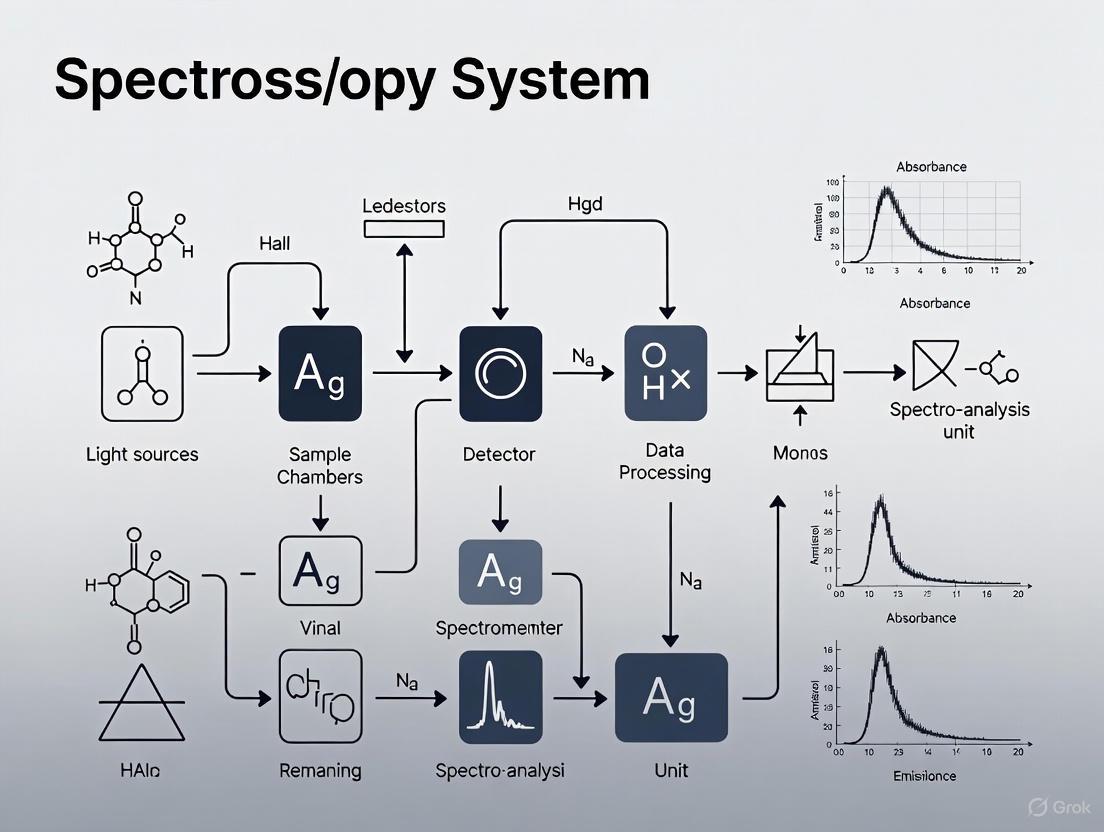
The process of conducting spectroscopic analysis and optimizing the system involves a logical sequence of steps, from sample preparation to data interpretation and system refinement. The workflow below visualizes this integrated process.
Diagram 1: Spectroscopy analysis workflow
The Scientist's Toolkit: Key Research Reagent Solutions
The following table details essential materials and software solutions used in advanced spectroscopic studies, particularly those involving novel fluorophores and microcavities as described in the protocols.
Table 4: Essential Research Reagents and Materials for Advanced Spectroscopic Studies
| Item Name | Function/Description | Application Example |
|---|---|---|
| Single Benzene Fluorophores (SBFs) | Donor-acceptor substituted benzene cores acting as highly emissive organic materials with high quantum yields in both solution and solid states [4]. | TGlu fluorophore for waveguiding and photocatalysis studies. |
| Dielectric Mirror Precursors | Polymer or colloidal solutions used to create highly reflective mirrors via spin-coating or dip-coating for microcavity fabrication [3]. | Building solution-processed optical microcavities. |
| Polariton Microcavity | A structure that confines light, enhancing its interaction with matter to form hybrid light-matter particles (polaritons) for quantum studies [3]. | Studying strong light-matter coupling and quantum phenomena. |
| Spectroscopy Software with AI/ML Modules | Software incorporating machine learning algorithms for automated spectral analysis, peak identification, and data interpretation from large datasets [5] [2]. | High-throughput analysis, spectral pattern recognition. |
| ICP-OES Vertical Plasma Systems | Spectrometers with vertical plasma orientation for enhanced matrix tolerance and lower detection limits for trace metal analysis [7]. | Environmental monitoring of heavy metals; semiconductor purity testing. |
Structural Thermal Optical Performance (STOP) Analysis Workflow
For high-power applications and systems operating in harsh environments (e.g., space telescopes, manufacturing lasers), it is critical to simulate how structural and thermal changes affect optical performance. STOP analysis is an engineering workflow used in the design stage to optimize systems for real-world conditions [8].
Diagram 2: STOP analysis for system robustness
Procedure for STOP Analysis:
Define Environmental Loads: In the simulation software (e.g., ANSYS Mechanical), specify the thermal and structural loads the system will encounter, such as in-orbit temperature variations for a CubeSat or heat generation from a high-power laser [8].
Perform Structural & Thermal Analysis: Run a Finite Element Analysis (FEA) to calculate the resulting structural deformations and temperature distributions throughout the optical system.
Map Data to Optical Model: Export the resulting surface deformations and refractive index gradient data from the FEA and map them onto the corresponding components in the optical design software (e.g., ANSYS Optical Studio).
Ray Tracing & Wavefront Analysis: Perform a ray trace through the deformed optical system. Analyze key metrics such as the wavefront error, spot diagram, and beam profile at the image or focal plane.
Evaluate System Performance: Assess whether the system still meets performance requirements (e.g., maintaining a specific beam size or focal point) under the applied environmental loads.
Optimize Design: If performance is degraded, iteratively adjust the mechanical design, material choices, or support structures and repeat the analysis until the system performs robustly in all expected conditions.
Outcome Metrics: STOP analysis prevents costly redesigns and failures by ensuring optical systems maintain their performance specifications after being exposed to real-world structural and thermal stresses, a critical step for manufacturability and reliability [8].
In modern spectroscopy, the journey from conceptual design to a functional, optimized system relies heavily on advanced optical simulation and analysis software. These tools enable researchers and engineers to bypass traditional, costly cycles of physical prototyping and testing, thereby accelerating development and enhancing performance. This Application Note provides a detailed comparison of three prominent software packages—Ansys Speos, TracePro, and Bruker OPUS—framed within the context of designing and optimizing spectroscopy systems for drug development and scientific research. While Speos and TracePro are powerful simulation tools for the design and virtual prototyping of optical systems, OPUS serves as the dedicated platform for operating spectroscopic instruments and analyzing acquired data [9] [10] [11]. This document will outline their distinct capabilities, provide protocols for their application, and illustrate their roles within the spectroscopy system lifecycle.
The table below summarizes the core attributes, primary strengths, and ideal application contexts for each software package, providing a high-level overview for selection.
| Software | Primary Function | Key Strengths | Typical Application Context in Spectroscopy |
|---|---|---|---|
| Ansys Speos [9] [12] | Optical system design & simulation | - Human Vision simulation- GPU acceleration (Live Preview)- Strong automotive & sensor (LiDAR) focus- Stray light analysis | - Design of illumination for sample analysis- Sensor (camera, LiDAR) integration and layout simulation- Assessing human-readable displays in spectroscopic instruments |
| TracePro [10] [13] [14] | Optical & illumination design & simulation | - Biomedical-specific features (tissue scattering, fluorescence)- Strong stray light analysis- Non-sequential ray tracing for complex systems | - Design and optimization of spectrometer optical trains (gratings, lenses, detectors)- Modeling light-tissue interaction for medical diagnostics- Minimizing noise via stray light analysis in sensitive systems |
| Bruker OPUS [11] [15] | Spectral data acquisition & analysis | - Direct instrument control for FT-IR, NIR, Raman- Validated for cGMP/GLP/GAMP- Multivariate quantification (QUANT3) & library search | - Operating Bruker spectrometers- Processing and quantifying spectral data (e.g., QUANT3 with SVR/LR algorithms)- Ensuring regulatory compliance in pharmaceutical labs |
For researchers, the choice between these tools is not mutually exclusive. Speos and TracePro are design and simulation tools used during the R&D and engineering phase to create and model the physical spectrometer. In contrast, OPUS is an operational and data analysis software used to run the instrument and interpret results after the hardware is built. The following visualization maps the logical workflow of a spectroscopy project, showing the complementary roles of simulation and operational software.
Detailed Capabilities for Spectroscopy
Ansys Speos
Speos excels in the design and validation of optical systems, with a strong emphasis on real-world performance and perception. Its capabilities are crucial for developing the optical components and sensor integrations often found in advanced spectroscopic instruments.
- Core Simulation Engine: Speos uses a ray tracing and ray propagation engine to predict light propagation within a 3D model. A key differentiator is its Human Vision capability, which physiologically models the human eye's response to light, allowing for high-fidelity visualization of illumination, crucial for designing user interfaces on spectroscopic devices [9] [12].
- GPU Acceleration: The Speos Live Preview function, powered by NVIDIA GPUs, allows for real-time interactive simulation. This drastically cuts iteration time, enabling designers to see results from the beginning of a simulation and make immediate adjustments to optical properties [9].
- Key Spectroscopy Features:
- Stray Light Analysis: Tools like Light Expert allow users to visualize interactions between light and geometry to identify causes of ghost images, reflections, and stray light, which is critical for maintaining signal-to-noise ratio [9].
- Sensor Simulation: Speos can assess camera and LiDAR raw signals, enabling the virtual validation of sensor layout on vehicles or other platforms, which can be pertinent for field-deployed spectroscopic systems [9] [16].
- Material and Surface Properties: It can model complex surface behaviors, including measured spectral 3D BxDFs, and volume behaviors like spectral absorption and scattering [9].
TracePro
TracePro is a dedicated optical engineering tool renowned for its precision in modeling light propagation in complex systems, making it particularly suited for the intricate optical trains of spectrometers and biomedical devices.
- Core Simulation Engine: Its foundation is a powerful non-sequential ray tracing engine, which is essential for simulating the complex paths of light in spectroscopy systems, including multiple reflections, refraction, scattering, and diffraction [10] [13].
- Biomedical and Spectroscopy Features:
- Material and Tissue Modeling: TracePro can model light scattering within biological tissues, a critical capability for designing medical diagnostic devices like those used in diffuse optical tomography or fluorescence-guided surgery [14].
- Diffractive Optical Elements (DOEs): It includes specialized tools for modeling holographic optical elements (HOEs) and computer-generated holograms (CGHs), which are essential for dispersing light in grating-based spectrometers [13].
- Comprehensive Stray Light Analysis: The software includes a dedicated Stray Light Analyzer to identify and eliminate ghost reflections and unwanted light paths, directly improving the signal-to-noise ratio in spectral measurements [13].
- Fluorescence and Polarization: It allows for detailed modeling of fluorescence effects (excitation and emission) and polarization effects, which are fundamental to techniques like fluorescence spectroscopy and polarization-sensitive imaging [10] [14].
Bruker OPUS
OPUS is not a system design tool but the operational software for Bruker's spectroscopy instruments. It is the platform for acquiring, processing, and evaluating spectral data, and is a standard in many industrial and research laboratories.
- Core Functionality: OPUS provides state-of-the-art measurement, processing, and evaluation of IR, NIR, and Raman spectra. It is a validated software prepared for operation in regulated environments compliant with cGMP/GLP/GAMP [11].
- Advanced Data Analysis Features:
- Multivariate Quantification (QUANT3): The latest version, OPUS 9.2, includes the QUANT3 package for developing multivariate calibrations. It introduces new algorithms like Support Vector Regression (SVR) and Local Regression (LR) to handle heterogeneous data sets and non-linearities more effectively than traditional PLS [15].
- Project-Based Design: QUANT3 uses a project-based structure, storing all models, spectra, and results in a single file to simplify data management and validation [15].
- Library Search and Identification: It offers advanced library search capabilities for the identification of unknown substances, including a new Autonomous Composition Identifier (A.I.D.) in OPUS-TOUCH for analyzing complex mixtures [11] [15].
Experimental Protocols
Protocol: Designing a Spectrometer Optical Train Using TracePro
This protocol outlines the methodology for designing and optimizing the core optical path of a Raman spectrometer using TracePro's non-sequential ray tracing capabilities [13] [14].
1. Objective: To model the excitation, scattering, and collection pathways of a Raman spectrometer to maximize signal collection efficiency and minimize stray light at the detector.
2. Research Reagent Solutions (Virtual Components):
| Component | Function in Simulation |
|---|---|
| Laser Source | Models the excitation wavelength, divergence, and spatial profile. |
| Sample Volume | Defines optical properties (absorption, scattering) to simulate Raman scattering and tissue interaction. |
| Collection Lenses/Mirrors | Guides scattered light onto the diffraction grating; performance is optimized for minimal aberration. |
| Diffraction Grating | Disperses collected light by wavelength; modeled as a diffractive optical element (DOE). |
| Detector | A virtual sensor that captures the dispersed spectrum and measures irradiance. |
3. Procedure:
- Step 1: Geometry Import/Creation. Import the CAD model of the spectrometer housing and optical components or create the geometry directly within TracePro.
- Step 2: Define Optical Properties. Assign precise surface and material properties to all components. For the diffraction grating, define its groove density and efficiency. For the sample, apply scattering and absorption coefficients representative of the target biological tissue [14].
- Step 3: Configure Light Source. Set up the laser source with the correct wavelength, power, and spatial characteristics. Define the Raman emission from the sample as a secondary, wavelength-shifted source.
- Step 4: Run Non-Sequential Ray Trace. Execute the ray trace simulation with a sufficient number of rays to achieve statistically significant results at the detector.
- Step 5: Stray Light Analysis. Use the Stray Light Analyzer tool to identify and trace paths of unwanted light (e.g., from ghost reflections or scatter) that reach the detector. Introduce baffles or apply anti-reflective coatings in the model to mitigate this noise [13].
- Step 6: Analyze and Optimize. Review the irradiance map on the detector. Evaluate signal strength and spectral resolution. Iteratively adjust the positions and curvatures of collection optics to maximize signal collection and uniformity.
The workflow for this design and optimization process is illustrated below.
Protocol: Validating Material Optical Properties with Ansys Speos
This protocol describes how to use Ansys Speos to validate the optical properties of a material used within a spectroscopic instrument, such as a housing coating to minimize stray light [9] [12].
1. Objective: To simulate and measure the reflectance and absorption properties of a material sample under controlled illumination to verify its suitability for reducing internal stray light.
2. Research Reagent Solutions (Virtual Components):
| Component | Function in Simulation |
|---|---|
| Standard Illuminant | Provides a controlled, spectrally defined light source (e.g., D65). |
| Material Sample | A virtual sample with assigned surface properties (e.g., BSDF) from a measured database. |
| Imaging Sphere Sensor | A simulated integrating sphere to capture hemispherical reflectance. |
| Luminance Camera Sensor | Provides a human-vision-based view of the material's appearance. |
3. Procedure:
- Step 1: Build Virtual Setup. In the Speos 3D environment, create a simple scene with the standard illuminant, the material sample plate, and the imaging sphere sensor.
- Step 2: Assign Material. Apply the material under test from the Speos custom materials library. This material should have pre-defined optical properties, such as a measured BSDF (Bidirectional Scattering Distribution Function).
- Step 3: Configure Simulation. Set up the simulation to run in the desired spectral range (e.g., Visible, NIR). Activate the Human Vision option if assessing visual appearance is required.
- Step 4: Run GPU-Accelerated Simulation. Execute the simulation using Speos Live Preview on an NVIDIA GPU for rapid iterative results.
- Step 5: Analyze Results. Examine the results in the post-processing tool. Quantify the total hemispherical reflectance from the imaging sphere sensor. Use the Light Expert tool to visualize specific light paths contributing to reflection and identify potential stray light contributors.
Protocol: Quantitative Analysis of Pharmaceutical Formulations using OPUS
This protocol details the steps for developing and using a multivariate calibration model in Bruker OPUS to quantify active pharmaceutical ingredient (API) concentration in a tablet [11] [15].
1. Objective: To create and validate a quantitative model (QUANT3) using NIR spectra to predict the concentration of an API in a solid dosage form.
2. Research Reagent Solutions:
| Component | Function |
|---|---|
| Bruker FT-NIR Spectrometer | Instrument for acquiring spectral data, controlled by OPUS. |
| Calibration Set Tablets | Tablets with known, varying API concentrations (reference values). |
| Validation Set Tablets | An independent set of tablets for testing the model's predictive accuracy. |
3. Procedure:
- Step 1: Spectral Acquisition. Using the OPUS software, measure the NIR spectra of all tablets in the calibration and validation sets under consistent operational parameters.
- Step 2: Data Preparation and Pre-processing. In the QUANT3 interface, load the spectra of the calibration set. Perform necessary spectral pre-processing (e.g., vector normalization, derivative) to enhance the spectral features related to the API.
- Step 3: Model Development. Assign the known reference values (API concentrations) to the corresponding spectra. Select an algorithm (PLS, SVR, or Local Regression) and allow OPUS to build the calibration model. The software will automatically handle dataset splitting (e.g., using the Kennard-Stone algorithm) to create training and test sets for internal validation [15].
- Step 4: Model Validation. Validate the model's performance using the independent validation set. OPUS will provide figures of merit such as the Root Mean Square Error of Prediction (RMSEP) and the coefficient of determination (R²).
- Step 5: Deploy for Prediction. Once validated, the model can be used within OPUS to predict the API concentration in unknown tablet samples routinely.
The workflow for this quantitative analysis is methodically outlined in the following diagram.
The effective design and optimization of modern spectroscopy systems require a suite of specialized software tools, each playing a distinct and critical role. Ansys Speos and TracePro are powerful allies in the virtual design and prototyping phase, enabling engineers to simulate optical performance, predict interactions, and eliminate costly errors before physical manufacturing. Speos brings strengths in human-centric visualization and sensor simulation, while TracePro offers unparalleled precision for modeling complex optical paths and biomedical interactions. Once a system is realized, Bruker OPUS takes the lead as a robust and compliant platform for instrument control, spectral acquisition, and advanced quantitative analysis, directly supporting research and quality control in demanding fields like pharmaceutical development. By understanding the capabilities and synergies between these platforms, researchers and scientists can make informed decisions that streamline the entire spectroscopy system lifecycle, from initial concept to final analytical results.
Optical spectroscopy software is a specialized tool designed to work with spectrometers for the collection, analysis, and interpretation of spectral data. It serves as the foundation of smart technologies that can determine the composition of any given material, enabling researchers to acquire data, gather information, and produce reports for better decision-making [17]. The global spectroscopy software market, valued at approximately USD 1.1 to 1.2 billion in 2024, is projected to grow at a compound annual growth rate (CAGR) of 9.1% to 9.2%, reaching around USD 2.5 billion by 2033-2034 [17] [1]. This growth is largely driven by increasing demand from the pharmaceutical industry, stringent environmental and food safety regulations, and continuous technological advancements [17].
For researchers, scientists, and drug development professionals, selecting the appropriate spectroscopy software is a critical decision that directly impacts data integrity, workflow efficiency, and regulatory compliance. This application note establishes a structured framework for evaluation based on three pivotal criteria: accuracy, CAD integration, and application-specific features, contextualized within the broader objective of designing and optimizing spectroscopy systems.
Core Selection Criteria and Evaluation Protocols
Accuracy and Performance Validation
Definition and Importance: Accuracy in spectroscopy software refers to the precision of data collection, processing, and interpretation. It ensures that spectral data reliably reflects the true composition and properties of the sample, which is non-negotiable in applications like drug development where decisions directly impact product safety and efficacy [6].
Quantitative Benchmarks: The following table summarizes key quantitative benchmarks for assessing software accuracy.
Table 1: Key Quantitative Benchmarks for Software Accuracy
| Performance Metric | Benchmark Value | Validation Method |
|---|---|---|
| Spectral Resolution | < 0.1 nm (UV-Vis) | Measurement of FWHM (Full Width at Half Maximum) of atomic emission lines [6]. |
| Peak Identification Accuracy | > 99.5% | Analysis of standard reference materials with known spectral peaks [6]. |
| Quantitative Analysis Error | < 1.0% RSD | Repeated measurement of standard concentrations for calibration curve validation [17]. |
| Algorithm Processing Speed | Millions of rays/sec (for optical simulation) | Ray tracing simulations on standardized hardware [18]. |
Experimental Protocol 1: Protocol for Validating Spectral Accuracy and Reproducibility
- Objective: To verify the software's accuracy in identifying known spectral features and its reproducibility across multiple measurements.
- Materials:
- Spectroscopy software under test (e.g., solutions from Thermo Fisher Scientific, Agilent Technologies, Bruker) [17].
- Calibrated spectrometer.
- Standard Reference Materials (SRMs): NIST-traceable holmium oxide filter (for wavelength accuracy) and a certified intensity standard.
- Procedure:
- System Calibration: Follow the software and instrument manufacturer's prescribed calibration procedure.
- Data Acquisition: Acquire spectra from the SRMs using three replicate measurements.
- Peak Analysis: Use the software's automated peak detection function to identify the characteristic peaks of the SRM.
- Data Comparison: Compare the software-identified peak positions (wavelengths) and intensities against the certified values from the SRM documentation.
- Statistical Analysis: Calculate the mean, standard deviation, and relative standard deviation (RSD) for the replicate measurements.
- Data Interpretation: The software is deemed to have passed the validation if the mean peak positions are within ±0.1 nm of the certified values and the RSD for intensity measurements is less than 1.0% [6].
Experimental Protocol 2: Protocol for Benchmarking Computational Performance
- Objective: To assess the software's efficiency in processing large spectral datasets, which is crucial for high-throughput screening in drug discovery [17].
- Materials:
- Spectroscopy software installed on a standardized workstation.
- A benchmark dataset comprising 10,000 spectral files.
- Procedure:
- Task Definition: Design a batch processing task that includes baseline correction, peak picking, and quantitative analysis.
- Execution: Execute the batch job and record the total processing time using the software's internal timer or an external stopwatch.
- Resource Monitoring: Use the operating system's resource monitor to track CPU and memory usage during the task.
- Data Interpretation: Compare the processing time and resource utilization against predefined project requirements or competing software solutions. Faster processing with stable resource usage indicates superior performance for high-throughput environments.
CAD and Software Ecosystem Integration
Definition and Importance: CAD integration refers to the software's ability to seamlessly interface with Computer-Aided Design (CAD) environments and other data management systems like LIMS (Laboratory Information Management Systems). This capability bridges the gap between mechanical design and optical analysis, enabling a cohesive workflow from component design to optical performance simulation [9] [18]. It reduces toolchain hand-offs, minimizes manual errors, and allows for early manufacturability evaluation, thereby accelerating the overall design cycle [19].
Evaluation Metrics: The table below outlines key metrics for evaluating integration capabilities.
Table 2: Metrics for Evaluating CAD and Ecosystem Integration
| Integration Feature | High-Quality Indicator | Application Benefit |
|---|---|---|
| Native CAD Plugin | Availability of a dedicated add-in (e.g., for SOLIDWORKS, Creo) [18]. | Allows application of optical properties and analysis directly within the CAD environment. |
| File Format Support | Robust import/export of STEP, SAT, IGES formats [18]. | Ensures compatibility and collaboration between mechanical and optical design teams. |
| LIMS/Data System Connectivity | Built-in connectors for automated data transfer to systems like LIMS [6]. | Streamlines data management, ensures traceability, and supports regulatory compliance (e.g., 21 CFR Part 11). |
| Scripting & Automation API | Access to a powerful macro or scripting environment (e.g., Scheme, Python) [18]. | Enables automation of repetitive tasks, creation of custom workflows, and extension of software capabilities. |
Experimental Protocol 3: Protocol for Testing CAD-to-Simulation Workflow Fidelity
- Objective: To validate the integrity and efficiency of transferring a CAD model into the spectroscopy or optical simulation software for analysis.
- Materials:
- CAD software (e.g., SOLIDWORKS).
- Spectroscopy/Optical software with claimed CAD integration (e.g., TracePro with its RayViz add-in for SOLIDWORKS) [18].
- Test model: A parametric CAD assembly of a simple optical mount or cuvette holder.
- Procedure:
- Model Preparation: Create or obtain the test model in the CAD environment.
- Export/Transfer: Use the software's integrated plugin or standard file format (e.g., STEP) to transfer the model.
- Fidelity Check: In the optical software, verify that all geometric features, dimensions, and assemblies are preserved and accurately represented.
- Optical Property Assignment: Apply material optical properties (e.g., refractive index, absorption) to the components within the optical software or via the CAD plugin.
- Simulation Execution: Run a basic ray-tracing or spectral simulation.
- Data Interpretation: A successful integration is demonstrated by a seamless transfer without geometry loss, the correct assignment and application of optical properties, and the successful execution of a simulation without errors attributable to the CAD model.
Application-Specific Features for Drug Development
Definition and Importance: Application-specific features are specialized functionalities that cater directly to the workflows, regulatory requirements, and analytical challenges of a particular sector. For pharmaceutical professionals, this includes capabilities for drug quality assurance, high-throughput screening, and regulatory compliance [17] [6].
Key Feature Analysis: The following table details critical application-specific features for the pharmaceutical industry.
Table 3: Essential Application-Specific Features for Pharmaceutical Drug Development
| Feature Category | Specific Software Capabilities | Impact on Pharmaceutical Workflows |
|---|---|---|
| Quantitative Analysis | Advanced chemometrics, multivariate calibration, and concentration prediction models [6]. | Enables precise determination of active pharmaceutical ingredient (API) concentration and impurity levels. |
| Compliance & Data Integrity | Audit trails, electronic signatures, user access controls, and compliance with 21 CFR Part 11 [6]. | Ensures data is reliable and traceable, meeting strict FDA and EMA regulatory standards for drug approval. |
| High-Throughput Screening | Automated batch processing, data visualization tools, and compatibility with microplate readers [17]. | Accelerates drug discovery by allowing rapid analysis of large compound libraries. |
| Material Identification & Purity | Spectral library searching, principal component analysis (PCA), and conformity tests [6]. | Verifies the identity and purity of raw materials and excipients, preventing defects and ensuring product safety. |
Experimental Protocol 4: Protocol for Evaluating a Pharmaceutical Quality Control Workflow
- Objective: To test the software's end-to-end capability in a simulated pharmaceutical quality control scenario for drug composition verification [6].
- Materials:
- Spectroscopy software with pharmaceutical analysis features.
- Spectrometer.
- Samples: API standard, excipient, and a batch of formulated tablets.
- Procedure:
- Method Development: Create an analytical method in the software. This includes building a calibration curve using the API standard at different concentrations.
- Library Management: Add reference spectra of the API and excipients to the software's spectral library.
- Sample Analysis: Acquire spectra from the tablet samples and run the pre-defined method.
- Automated Reporting: Use the software's reporting module to generate a compliance report that includes the identified components, quantified API concentration, and any spectral anomalies.
- Data Interpretation: The software is evaluated on its ability to correctly identify the API and excipients via library search, accurately quantify the API concentration against the calibration curve and flag any outliers or spectral mismatches that could indicate impurities or formulation errors.
The Scientist's Toolkit: Essential Research Reagent Solutions
The following table lists key materials and software solutions essential for experiments in this field.
Table 4: Key Research Reagent Solutions for Spectroscopy System Optimization
| Item | Function / Application |
|---|---|
| NIST-Traceable Standard Reference Materials (SRMs) | Provides an absolute benchmark for validating the wavelength and photometric accuracy of the spectroscopy system [6]. |
| Optical Spectroscopy Software (e.g., from Thermo Fisher, Agilent, Bruker) | Core platform for data acquisition, processing, analysis, and reporting; enables material characterization and quality control [17] [6]. |
| CAD-Integrated Optical Software (e.g., Ansys Speos, TracePro) | Facilitates the design and virtual validation of optical components and systems within a CAD environment, reducing prototyping needs [9] [18]. |
| Parametric CAD Model of Spectrometer Component | Serves as a digital twin for simulating optical paths, component integration, and performing virtual tolerance analysis [19] [18]. |
| Scripting Macro (e.g., Scheme, Python) | Automates repetitive software tasks, customizes analysis routines, and enhances workflow efficiency and reproducibility [18]. |
Workflow Visualization
The following diagram illustrates the logical workflow for selecting and validating spectroscopy software based on the key criteria discussed.
Software Selection and Validation Workflow
This diagram outlines a systematic, iterative process for selecting optical spectroscopy software. It begins with clearly defining system requirements, followed by concurrent evaluation of the three core criteria: Accuracy, CAD Integration, and Application-Specific Features. Each criterion is assessed through specific experimental protocols. The results feed into a final decision point; if the software fails any criterion, the process loops back to requirement definition, ensuring a rigorous and comprehensive selection process.
Defining System Requirements for Pharmaceutical and Clinical Applications
Core System Requirements for Pharmaceutical Spectroscopy
Designing spectroscopy systems for pharmaceutical and clinical applications requires a meticulous approach to ensure data integrity, regulatory compliance, and analytical precision. The core requirements span hardware, software, and operational protocols.
System Qualification & Compliance Requirements
All spectroscopic instruments intended for regulated environments must undergo a rigorous qualification and validation process. The requirements can be categorized as follows:
Table 1: System Qualification & Compliance Requirements
| Requirement Category | Description | Key Standards & Examples |
|---|---|---|
| System Qualification | A three-tiered process to verify instrument performance [20]. | Design Qualification (DQ): Verifies the instrument's design attributes are acceptable.Operational Qualification (OQ): Confirms adherence to intended use specifications.Performance Qualification (PQ): Defines instrument's intended performance for specific applications [20]. |
| Software Compliance | Software must ensure data integrity and security [21]. | 21 CFR Part 11 / EU Annex 11: Mandates electronic signatures, audit trails, and unique user log-ins. Software like Vision Air fulfills these technical requirements [21]. |
| Pharmacopoeia Compliance | Instruments must adhere to established testing protocols for their intended use [20]. | Adherence to USP, European, Japanese, or Chinese pharmacopoeias. Automated software tests adhering to NIST standards, such as the polystyrene standard in FTIR, are essential [20]. |
| Operator Training | Formalized processes are required to ensure operators are competent [20]. | Crucial for maintaining standardized operations and data credibility [20]. |
Application-Specific Technical Requirements
The technical specifications of a spectroscopy system are dictated by its specific application within the pharmaceutical workflow, from raw material inspection to final product quality assurance.
Table 2: Application-Specific Technical Requirements
| Application | Technology | Key System Requirements |
|---|---|---|
| Raw Material Identification | NIR Spectroscopy [21], Raman Spectroscopy [22] | Portability for use in warehouses [21]. Spatial resolution and molecular specificity for verifying API and excipient identity and purity [22]. |
| Polymorph & Crystallinity Characterization | Raman Spectroscopy [22] | High sensitivity and spectral resolution to differentiate between polymorphic forms that influence drug solubility and efficacy [22]. |
| Inline/Online Process Control | NIR Spectroscopy [21] | Real-time monitoring capability, fiber optic probes, ruggedized design for manufacturing environments, and software for real-time data analysis [21]. |
| Content Uniformity & Blend Homogeneity | NIR Spectroscopy [21], Raman Chemical Mapping [22] | For NIR: Rapid measurement of multiple tablets simultaneously [21]. For Raman: Confocal microscopy for detailed chemical mapping of API distribution within a tablet [22]. |
| Finished Product Quality Assurance | NIR Spectroscopy [21], FTIR Spectroscopy [20] | Non-destructive analysis, ability to analyze products in blisters, and determine multiple parameters (e.g., content, dissolution profile, hardness) [21]. FTIR must provide data on identity, purity, and quantity [20]. |
Experimental Protocols
Protocol: Raw Material Identity Verification using Handheld NIR Spectroscopy
This protocol outlines the procedure for the rapid, non-destructive identification of incoming raw materials (APIs, excipients) in a pharmaceutical warehouse or weighing area [21].
Workflow
The following workflow illustrates the procedural and data integrity steps for raw material verification.
Materials and Equipment
Table 3: Research Reagent Solutions & Essential Materials
| Item | Function |
|---|---|
| Handheld or Portable NIR Spectrometer | Allows for rapid, on-site analysis of materials without the need to transport samples to a central lab [21]. |
| 21 CFR Part 11 Compliant Software | Ensures data integrity through user authentication, electronic signatures, and a complete, uneditable audit trail [21]. |
| Qualified Spectral Library | A validated database of reference spectra for all approved raw materials, used by the software to compare and identify unknown samples [21]. |
| Vial or Bag of Raw Material | The sample to be tested, often analyzed directly in its container with minimal or no preparation [21]. |
Protocol: Tablet Content Uniformity and Chemical Mapping using Confocal Raman Microscopy
This protocol uses Confocal Raman Microscopy to non-destructively assess the distribution and identity of the Active Pharmaceutical Ingredient (API) within a solid dosage form, providing critical information for formulation development and quality control [22].
Workflow
The workflow details the steps from sample mounting to image generation for analyzing component distribution within a tablet.
Key Methodology Details
- Spatial Resolution: The confocal design enables chemical analysis with microscale spatial resolution, allowing visualization of individual API particles and excipients [22].
- Non-Destructive Analysis: The sample remains intact after analysis, allowing for further testing or archival, which is crucial for expensive APIs or limited-quantity samples [22].
- Polymorph Identification: The high molecular specificity of Raman spectroscopy allows it to differentiate between different crystalline forms (polymorphs) of the API, which is critical for predicting drug performance [22].
- Regulatory Compliance: Systems should include 21 CFR Part 11 compliant software to support method validation and data integrity requirements for use in regulated environments [22].
Protocol: Inline Process Monitoring of Granulation using NIR Spectroscopy
This protocol describes the use of an inline NIR probe to monitor a granulation process in real-time, enabling proactive control of Critical Process Parameters (CPPs) and supporting Quality by Design (QbD) and PAT initiatives [21].
Workflow
The workflow illustrates the continuous feedback loop of real-time data acquisition and process control.
Key Methodology Details
- Real-Time Monitoring: The NIRS XDS Process Analyzer fitted with a fiber optic probe can monitor parameters like residual solvent and water content in powders and granulates in real-time, reducing material loss and maximizing time efficiency [21].
- Multivariate Modeling: The system relies on pre-calibrated multivariate models (e.g., PLS regression) that correlate spectral data to reference values for moisture and concentration [21].
- PAT Integration: This methodology is a core component of the FDA's Process Analytical Technology (PAT) initiative, which encourages real-time quality control to ensure final product quality [21].
Building and Simulating Systems: From Raman to Hyperspectral Imaging
The design and optimization of modern spectroscopy systems rely on a tightly coupled workflow between virtual modeling and experimental validation. This integrated approach allows researchers and drug development professionals to predict optical performance, refine system parameters, and significantly reduce prototyping costs and development time. The process typically begins with computational modeling of the molecular system or optical setup, proceeds through virtual simulation of spectroscopic results, and culminates in experimental validation using advanced instrumentation. This methodology is particularly valuable in pharmaceutical applications where precision in material identification and quality assurance is critical [6] [9]. Advanced optical design software like Ansys Speos now enables researchers to simulate a system's optical performance and evaluate final illumination effects based on human vision capabilities, creating a seamless bridge between virtual prototyping and physical realization [9].
Computational Modeling and Molecular Dynamics
Molecular Environment Characterization
The foundation of accurate spectroscopic simulation begins with realistic modeling of molecular environments. Classical molecular dynamics (MD) simulations generate the atomic-level trajectories and configurations that represent the system's behavior over time. For complex molecular systems with nanoscopic heterogeneities—such as drug compounds in multi-component solutions—this step is crucial for capturing the intricate molecular arrangements that arise from diverse interactions among components [23].
The Instantaneous Frequencies of Molecules (IFM) method represents a significant advancement in this area. This parameter-free methodology couples with classical MD simulations to predict vibrational observables, including the Frequency Fluctuation Correlation Function (FFCF) and solvatochromic shifts. When applied to N-methylacetamide (NMA) in seven different chemical environments, the IFM method demonstrated strong agreement with experimental results for both NMA solvatochromism and FFCF dynamics, including characteristic times and amplitudes of fluctuations [23].
Table: Key Components for Computational Modeling
| Research Reagent/Component | Function in Workflow |
|---|---|
| Molecular Dynamics (MD) Simulation Software | Generates atomic trajectories and configurations of the molecular system over time |
| GFN2-xTB Semiempirical Method | Calculates vibrational frequencies with low computational cost while maintaining accuracy |
| Frequency Maps | Transforms molecular coordinates into spectroscopic observables like instantaneous frequencies |
| N-methylacetamide (NMA) | Model compound for validating computational methodologies via its sensitive amide I vibrational mode |
| Solvent Environments (D2O, DMSO, etc.) | Provide varied chemical environments for testing computational method transferability |
Computational Protocol
Protocol 1: Molecular Dynamics with Instantaneous Frequency Calculation
- System Preparation: Construct initial coordinates of the solute molecule (e.g., N-methylacetamide) and solvent boxes representing the chemical environments of interest. Energy-minimize the initial structure to remove steric clashes [23].
- Force Field Parameterization: Apply appropriate classical force fields to all components. Ensure the force field accurately describes non-covalent interactions, which are critical for simulating spectroscopic observables [23].
- Equilibration Phase: Run the MD simulation under the desired thermodynamic conditions (NPT or NVT ensemble) until system properties (density, potential energy) stabilize. This typically requires 1-5 nanoseconds depending on system complexity [23].
- Production Phase: Execute a multi-nanosecond MD simulation, saving molecular coordinate snapshots at regular intervals (e.g., every 100 fs) for subsequent frequency analysis.
- Instantaneous Frequency Calculation: For each saved snapshot, extract the solute molecule and its surrounding solvation shells. Use the GFN2-xTB semiempirical method to compute the vibrational spectrum and extract the frequency of the specific vibrational mode of interest [23].
- Data Analysis: Calculate the average frequency (for linear IR) and construct the frequency-frequency time correlation function to obtain the FFCF for comparison with 2DIR experiments [23].
Optical System Simulation
Monte Carlo Methods for Light Transport
For simulating how light propagates through biological samples or optical components, Monte Carlo (MC) methods provide a powerful stochastic approach to solving the radiative transfer equation. These simulations model key light-tissue interaction mechanisms including absorption, elastic scattering, fluorescence, and Raman scattering. A recently developed spectroscopic MC package enables researchers to simulate all these competing phenomena simultaneously, providing a comprehensive platform for predicting depth-resolved spectroscopic signals [24].
MC methods are particularly valuable for designing and optimizing fiber-optic probes used in biomedical Raman spectroscopy. These simulations can establish rigorous relationships between Raman sensing depth and tissue optical properties, which is essential for developing clinically viable systems. For instance, MC simulations have demonstrated that for a realistic Raman probability of 10⁻⁶, the sensing depth ranges between 10 and 600 μm for absorption coefficients of 0.001 to 1.4 mm⁻¹ and reduced scattering coefficients of 0.5 to 30 mm⁻¹ [24].
Table: Quantitative Analysis of Raman Sensing Depth via Monte Carlo Simulation
| Absorption Coefficient (mm⁻¹) | Reduced Scattering Coefficient (mm⁻¹) | Raman Sensing Depth (μm) |
|---|---|---|
| 0.001 | 1 | 105-225 |
| 0.001-1.4 | 0.5-30 | 10-600 |
| Values obtained for a realistic Raman probability of 10⁻⁶ [24] |
Optical Simulation Protocol
Protocol 2: Monte Carlo Simulation of Spectroscopic Signals
- Optical Property Definition: Specify the absorption coefficient (μₐ), scattering coefficient (μₛ), anisotropy factor (g), and refractive index (n) for all materials in the simulation domain [24].
- Source Configuration: Define the light source parameters including wavelength, beam diameter, numerical aperture, and incident angle. For Raman simulations, incorporate the appropriate Raman probability (typically 10⁻⁶ for biological tissues) [24].
- Geometry Construction: Create a digital model of the sample geometry. This can range from simple layered structures to complex voxel-based representations of heterogeneous tissues [24].
- Photon Launching: Simulate photon propagation through the medium using stochastic sampling of interaction probabilities. Track photon weight, position, and direction after each scattering event [24].
- Interaction Handling: At each step, determine whether absorption, elastic scattering, fluorescence, or Raman scattering occurs based on the relative probabilities of each process [24].
- Signal Collection: Implement virtual detectors to record the desired spectroscopic signals (e.g., Raman photons within a specific wavelength shift) based on their position and trajectory [24].
- Data Analysis: Process the collected photons to generate predicted spectra or spatial maps of the spectroscopic signal, including depth-resolved information [24].
Experimental Validation and Instrumentation
Spectroscopic Instrumentation for Validation
The final phase of the workflow involves validating computational predictions using advanced spectroscopic instrumentation. Recent innovations in this domain show a distinct trend toward field-portable devices and specialized laboratory systems with enhanced capabilities. The 2025 review of spectroscopic instrumentation highlights several cutting-edge technologies relevant to pharmaceutical and research applications [25].
Fluorescence instrumentation has seen specialized developments like the Veloci A-TEEM Biopharma Analyzer from Horiba, which simultaneously collects absorbance, transmittance, and fluorescence excitation-emission matrix (A-TEEM) data. This provides an alternative to traditional separation methods for characterizing monoclonal antibodies, vaccines, and protein stability [25].
In Raman spectroscopy, new systems include the PoliSpectra rapid Raman plate reader designed for fully automated measurement of 96-well plates, addressing the needs of pharmaceutical and biopharmaceutical markets with high-throughput screening tools. For hazardous materials identification, the TaticID-1064ST handheld Raman spectrometer offers analysis guidance with onboard documentation features [25].
Mid-infrared spectroscopy continues to advance with systems like the Bruker Vertex NEO platform, which incorporates a vacuum ATR accessory that maintains samples at normal pressure while keeping the entire optical path under vacuum. This effectively removes atmospheric interference, which is particularly beneficial for protein studies and far-IR research [25].
Experimental Validation Protocol
Protocol 3: Experimental Validation of Simulated Results
- Sample Preparation: Prepare standardized samples of the material system under investigation. For pharmaceutical applications, this may include drug compounds, excipients, or biological macromolecules in controlled solvent environments [25] [23].
- Instrument Calibration: Perform standard calibration procedures using reference materials specific to the spectroscopic technique being employed (e.g., polystyrene for IR, cyclohexane for Raman) [25].
- Data Acquisition: Collect spectroscopic data using the appropriate instrument configuration. For comparison with dynamics simulations, 2DIR spectroscopy may be employed to measure the FFCF directly [23].
- Spectral Processing: Apply necessary preprocessing steps including baseline correction, normalization, and noise reduction to the experimental spectra [6].
- Quantitative Comparison: Compare experimental results with computational predictions using statistical metrics. For IR spectroscopy, this includes analyzing solvatochromic frequency shifts and FFCF parameters (characteristic times and amplitudes) [23].
- Model Refinement: If discrepancies exist between simulation and experiment, iteratively refine the computational models (e.g., force field parameters, optical properties) to improve agreement [23].
- Validation Reporting: Document the degree of agreement between simulated and experimental results, including uncertainty estimates and limitations of both approaches.
Table: Selected Advanced Spectroscopic Instrumentation (2024-2025)
| Instrument | Technique | Key Features | Applications |
|---|---|---|---|
| Veloci A-TEEM Biopharma Analyzer | Fluorescence (A-TEEM) | Simultaneous absorbance, transmittance, fluorescence EEM | Monoclonal antibodies, vaccine characterization |
| Vertex NEO Platform | FT-IR | Vacuum ATR accessory, multiple detector positions | Protein studies, far-IR research |
| PoliSpectra | Raman | Automated 96-well plate reading, liquid handling | High-throughput screening in pharma |
| SignatureSPM | Raman/Photoluminescence | Integrated scanning probe microscope | Semiconductors, nanotechnology |
| BrightSpec MRR | Microwave | Broadband chirped pulse microwave spectrometer | Molecular structure determination |
Non-Sequential Ray Tracing for Complex Optical Paths and Stray Light Analysis
Non-sequential ray tracing is a powerful simulation methodology that allows optical engineers to model the behavior of light without requiring rays to follow a predefined sequence of optical surfaces [26]. Unlike sequential ray tracing, where rays are confined to propagate from one defined surface to the next in a specific order, non-sequential modeling enables rays to interact with optical components in any order, with the capability to hit objects multiple times or not at all [26]. This fundamental characteristic makes it particularly valuable for analyzing complex optical phenomena where light paths are not easily predictable, such as stray light analysis, ghost reflections, and illumination system design.
Within optical design software like Zemax OpticStudio, non-sequential ray tracing operates by modeling optical components as true three-dimensional objects, including both surfaces and solid volumes [26]. Each object is positioned globally with independent x, y, z coordinates and orientation, allowing for accurate representation of real-world optical systems. This approach is essential for modeling complex components that cannot be accurately represented by single surfaces, including prisms, corner cubes, light pipes, and CAD-imported geometries [26]. For spectroscopy system optimization, this capability provides critical insights into light behavior throughout the entire optical path, enabling researchers to identify and mitigate performance-degrading effects before physical prototyping.
Fundamentals of Stray Light Analysis
Stray light refers to unwanted light in an optical system that can significantly degrade performance by introducing noise and reducing contrast [27]. In the context of spectroscopy systems used for drug development, stray light can compromise measurement accuracy, leading to unreliable data and potentially affecting research outcomes. Stray light manifests through several physical mechanisms, each with distinct characteristics and mitigation requirements.
- Reflections: These occur when light bounces off surfaces not intended to contribute to the signal. In spectroscopic instruments, internal surface reflections can create flare and ghosting effects that interfere with accurate spectral measurements, particularly in high-contrast scenarios [27].
- Scattering: This phenomenon results from light interacting with surface imperfections, contaminants, or roughness. Scattering causes a diffuse spread of light, potentially obscuring fine spectral features and reducing the system's overall signal-to-noise ratio [27]. This is particularly problematic in spectroscopy systems requiring high sensitivity.
- Diffraction: Diffraction occurs when light bends around edges or through small apertures, creating unwanted patterns that reduce spectral sharpness and clarity [27]. In spectrometers, diffraction from aperture edges can limit resolution and cause spectral cross-talk between adjacent channels.
The combined effects of these stray light sources can lead to reduced measurement contrast, false spectral signals, and decreased signal-to-noise ratio [27]. For pharmaceutical researchers relying on spectroscopic data for drug development, effective stray light control is not merely an optimization concern but a fundamental requirement for data integrity.
Software Tools and Implementation
Non-Sequential Ray Tracing in OpticStudio
Zemax OpticStudio provides two distinct modes for non-sequential analysis: Pure Non-Sequential Mode and Mixed Sequential/Non-Sequential Mode [26]. In Pure Non-Sequential Mode, all optical components reside in a single non-sequential group where sources and detectors are configured to launch and record rays. This mode offers comprehensive source modeling capabilities, allowing complex three-dimensional source distributions beyond the point sources available in sequential mode [26]. The software's ray tracing engine can handle ray splitting, scattering, and diffraction at phase surfaces, with analysis outputs including radiometric detector data and ray history databases.
Mixed Mode combines sequential and non-sequential capabilities, where non-sequential groups are embedded within a larger sequential system [26]. Sequentially traced rays enter the non-sequential group through an entrance port, interact with the three-dimensional components inside, then exit through an exit port to continue propagating through the sequential system. This approach is particularly valuable for spectroscopy systems that are fundamentally sequential but contain components better modeled as 3D volumes, such as complex sample cells, integrating spheres, or specialized filters.
Table 1: Non-Sequential Ray Tracing Modes in OpticStudio
| Mode Type | Key Features | Best Applications in Spectroscopy |
|---|---|---|
| Pure Non-Sequential | All components in non-sequential group; comprehensive source modeling; ray splitting and scattering | Illumination uniformity studies; complex component analysis; stray light mapping |
| Mixed Mode | Non-sequential groups embedded in sequential system; entrance and exit ports; sequential performance metrics | Systems with both imaging and non-sequential elements; spectrometers with complex sample compartments |
Specialized Stray Light Analysis Tools
TracePro stands as a specialized software solution for stray light analysis, employing Monte Carlo ray tracing to simulate light paths with high statistical accuracy [27]. Originally developed for NASA, TracePro includes advanced features such as path sorting and ray visualization tools essential for identifying significant stray light contributions in complex systems [27]. The software offers robust CAD integration capabilities, allowing users to import and analyze intricate mechanical geometries that might contribute to stray light through scattering or unintended reflections.
For spectroscopy systems, these software tools enable researchers to quantify stray light performance through metrics such as Point Source Normalized Irradiance Transmittance (PSNIT) and to identify critical surfaces contributing to stray light through path analysis. This capability is particularly valuable during the design phase of spectroscopic instruments for pharmaceutical applications, where regulatory requirements often demand rigorous characterization of measurement accuracy.
Table 2: Stray Light Analysis Software Capabilities
| Software Tool | Key Stray Light Features | Strengths for Spectroscopy Applications |
|---|---|---|
| Zemax OpticStudio | Non-sequential ray tracing; detector objects; ray database files; path analysis | Integration with sequential optical design; parametric optimization; sensitivity analysis |
| TracePro | Monte Carlo ray tracing; CAD integration; advanced path sorting; NASA-developed algorithms | Handling complex mechanical assemblies; statistical accuracy; specialized stray light visualization |
Quantitative Analysis and Performance Metrics
Effective stray light analysis requires quantifying performance through standardized metrics that enable objective comparison between design alternatives. The most common metric is the Point Source Normalized Irradiance Transmittance (PSNIT), which measures the system's response to an off-axis bright source relative to the in-axis signal. For spectroscopy systems, this is particularly important when measuring weak spectral features in the presence of strong nearby lines or when the instrument must operate with bright sources in its field of view.
In non-sequential ray tracing software, these quantitative assessments are typically performed using detector objects that capture irradiance distributions [26]. The detectors support various data types including incoherent irradiance, coherent irradiance, radiant intensity, and true color photometric results [26]. For spectroscopic applications, the spectral response can be characterized by configuring sources with specific wavelength distributions and analyzing detector response across wavelength bands.
Table 3: Key Stray Light Performance Metrics
| Metric | Definition | Application in Spectroscopy Systems |
|---|---|---|
| PSNIT (Point Source Normalized Irradiance Transmittance) | Ratio of stray light irradiance to input irradiance as a function of field angle | Quantifies susceptibility to off-axis light sources; critical for fluorescence spectroscopy |
| BSDF (Bidirectional Scattering Distribution Function) | Angular distribution of scattered light from a surface | Characterizes scattering from optical components; essential for low-light-level Raman spectroscopy |
| Ghost Reflection Intensity | Relative strength of unwanted reflections compared to primary signal | Important for high-dynamic-range absorption spectroscopy |
Experimental Protocols for Stray Light Analysis
Protocol 1: Baseline Stray Light Characterization
This protocol establishes a standardized methodology for quantifying stray light performance in spectroscopy systems using non-sequential ray tracing.
Materials and Equipment:
- Optical modeling software with non-sequential ray tracing capability (OpticStudio or TracePro)
- Complete system optical model including mechanical surfaces
- Computational resources adequate for Monte Carlo simulations
Procedure:
- Model Preparation: Ensure the optical model includes all significant optical and mechanical surfaces with appropriate optical properties assigned. Mechanical surfaces should have measured or estimated scatter properties based on surface finish.
- Source Definition: Configure a collimated source representing the input light to the spectroscopy system. For full system characterization, define multiple field points across the input aperture.
- Detector Placement: Position detector objects at key system locations, including the focal plane where the spectral dispersion occurs. Additional detectors may be placed at intermediate image planes and at critical mechanical surfaces to identify scattering sources.
- Ray Tracing: Execute a ray trace with sufficient rays to achieve statistical significance (typically 1,000,000+ rays for initial analysis). Use importance sampling if available to improve efficiency.
- Path Analysis: Utilize path sorting tools to identify the most significant stray light paths contributing to noise at the detector plane. Filter ray databases to isolate paths that involve multiple bounces or scattering events.
- Quantification: Calculate stray light metrics including PSNIT values for critical field angles and the total stray light contribution as a percentage of the primary signal.
Interpretation: Paths contributing more than 1% of the primary signal intensity should be flagged for mitigation. The analysis should prioritize paths that directly reach the detector plane over those that terminate elsewhere in the system.
Protocol 2: Scattering Surface Analysis
This protocol specifically characterizes the impact of surface roughness and contamination on stray light performance, critical for maintaining spectroscopy system reliability in pharmaceutical research environments.
Materials and Equipment:
- Surface scatter measurement data (if available)
- ABg scatter model parameters for typical surface finishes
- Software supporting bidirectional scattering distribution function (BSDF) models
Procedure:
- Surface Property Assignment: Apply appropriate scatter models to optical and mechanical surfaces based on their material properties and manufacturing specifications. Use measured BSDF data when available or industry-standard ABg parameters for typical surface finishes.
- Parametric Analysis: Vary surface roughness parameters across expected manufacturing tolerances to establish sensitivity of system performance to finish quality.
- Contamination Modeling: Introduce representative contaminant particles (dust, fingerprints) at critical surfaces with appropriate scattering properties to simulate real-world operating conditions.
- Comparative Ray Tracing: Execute identical ray traces for clean and contaminated states, maintaining constant ray counts for valid comparison.
- Detector Analysis: Quantify the increase in stray light noise at the detector plane attributable to surface scatter and contamination.
Interpretation: Surfaces contributing more than 0.1% additional stray light when contaminated should be identified for special handling procedures or design modification. The results inform cleaning protocols and tolerance specifications for critical surfaces.
Mitigation Strategies and System Optimization
Based on the identification of problematic stray light paths through non-sequential analysis, several mitigation strategies can be implemented to optimize spectroscopy system performance.
Optical Design Optimization
Surface treatments and optical design modifications represent the first line of defense against stray light. Anti-reflection coatings can be optimized for specific wavelength ranges used in pharmaceutical spectroscopy applications to reduce surface reflections that might otherwise contribute to ghost images [27]. Baffles and light traps can be strategically placed to intercept stray light paths before they reach critical components, with their effectiveness validated through non-sequential simulation before implementation.
For spectroscopy systems specifically, field stops and apertures can be positioned at image planes to limit the propagation of unwanted light, while pupil stops can control the range of ray angles proceeding through the system [28]. The historical effectiveness of these approaches is demonstrated by their continued use since Euler's recommendations in the 18th century for controlling "extraneous light" in optical systems [28].
Material and Surface Selection
The selection of appropriate materials and surface treatments plays a crucial role in stray light control. Black surface treatments with low reflectance properties should be applied to mechanical surfaces within the optical path, with specific attention to surfaces that are directly visible from the detector or from critical optical elements [28]. The performance of these treatments should be characterized by their Bidirectional Reflectance Distribution Function (BRDF) across the relevant wavelength range.
For spectroscopic instruments requiring the highest sensitivity, such as those used for detecting low-concentration analytes in drug development, specialized low-reflectance materials such as black anodized coatings, proprietary black paints, or structured black surfaces may be necessary for critical baffles and mounts. The effectiveness of these materials can be evaluated through non-sequential simulation by incorporating measured BRDF data into the optical model.
The Scientist's Toolkit: Essential Research Reagents and Materials
Table 4: Essential Tools for Stray Light Analysis and Control
| Tool Category | Specific Examples | Function in Stray Light Management |
|---|---|---|
| Software Solutions | Zemax OpticStudio, TracePro, CODE V | Non-sequential ray tracing simulation; path analysis; performance prediction |
| Surface Characterization | BRDF measurement instruments; surface profilometers; scatterometers | Quantify surface scattering properties; validate manufacturing quality |
| Optical Coatings | Anti-reflection coatings; metallic mirrors; protective coatings | Control surface reflections; enhance desired transmissions; protect vulnerable surfaces |
| Black Surface Treatments | Black anodize; Martin Black; Acktar Fractal Black; proprietary paints | Absorb stray light; prevent scattered light from reaching detector |
| Baffle Materials | Aluminum baffles with black treatment; 3D-printed light traps; serrated edges | Block direct paths for stray light; reduce scattering from baffle edges |
| CAD Software | SolidWorks, CATIA, Creo | Design mechanical housing; create geometries for import into optical software |
Non-sequential ray tracing provides an indispensable methodology for analyzing and mitigating stray light in spectroscopy systems critical to pharmaceutical research and drug development. By enabling comprehensive simulation of complex light paths that traditional sequential methods cannot capture, this approach allows optical designers to identify problematic stray light contributions early in the design process, reducing costly design iterations and performance compromises. The structured protocols and quantitative metrics outlined in this application note provide researchers with a validated framework for characterizing and optimizing spectroscopic instrumentation, ultimately supporting the development of more reliable and accurate analytical systems for the pharmaceutical industry. As spectroscopy continues to evolve toward higher sensitivity and greater precision, the role of non-sequential analysis in ensuring measurement integrity will only increase in importance.
The design of high-performance spectroscopy systems hinges on the effective integration of three core optical components: lenses, diffraction gratings, and detectors. For researchers and drug development professionals, optimizing these elements is critical for achieving reliable data in applications ranging from raw material identification to final product quality control [20]. The contemporary design process is increasingly reliant on advanced optical simulation software, which allows for precise modeling and optimization before physical prototyping, saving significant time and cost [13]. This application note details the function, selection criteria, and integration strategies for these key components within a modern, software-driven development framework.
The Crucial Dispersive Element: Diffraction Gratings
Fundamental Principles and Types
Diffraction gratings are the primary components for dispersing light into its constituent wavelengths in most spectrometers. They operate on the principle of diffraction, where a periodic microstructure of grooves causes light to interfere constructively at specific angles dependent on its wavelength [29] [30]. This is described by the grating equation: ( m\lambda = d(\sin\alpha + \sin\beta) ), where (m) is the diffraction order, (\lambda) is the wavelength, (d) is the groove spacing, (\alpha) is the incident angle, and (\beta) is the diffracted angle [29].
Gratings are broadly categorized by their physical operation and manufacturing method, each with distinct advantages as shown in Table 1.
Table 1: Comparison of Primary Diffraction Grating Types for Spectrometer Design
| Grating Type | Core Principle | Typical Groove Profile | Advantages | Common Applications |
|---|---|---|---|---|
| Ruled/Blazed Reflection [29] [30] | Light reflects off a grooved surface with a triangular profile. | Blazed (Triangular) | Superior efficiency at a specific "blaze" wavelength [29] [31]. | Monochromators, laser tuning [31] [30]. |
| Holographic Reflection [29] [30] | Grooves formed via an optical interference pattern (photolithography). | Sinusoidal | Reduced stray light and ghosts [29] [31]. | High-fidelity spectrographs, optical communications [31]. |
| Transmission [29] [31] | Light is diffracted while passing through a grooved substrate. | Blazed or Sinusoidal | Insensitive to polarization; enables compact, in-line optical paths [29] [31]. | Compact spectrometers, in-line process control. |
| Echelle [29] | Operates at high angles and orders with lower groove density. | Coarse, Blazed | Very high resolving power and dispersion [29]. | High-resolution astronomy, atomic spectroscopy [29]. |
Selection Criteria and Experimental Protocol
Protocol 2.1: Methodology for Selecting a Diffraction Grating
Objective: To systematically choose an optimal diffraction grating based on the spectroscopic application's requirements.
Materials:
- Light source (e.g., laser, broadband lamp)
- Sample holder and cell
- Optical breadboard and mounts
- Power meter or spectrometer for validation
Procedure:
- Define Spectral Range: Identify the wavelength range of interest (e.g., UV, Vis, NIR). Ensure the grating is coated for high efficiency across this range [30].
- Determine Required Resolution: Calculate the necessary resolving power ((R = \lambda / \Delta\lambda)). Use Equation 2, (R = mN), where (m) is the order and (N) is the number of illuminated grooves, to guide grating selection [29].
- Choose Grating Type: Based on Table 1:
- For high efficiency in a narrow band (e.g., laser line), select a blazed ruled grating.
- For broad spectral analysis with minimal stray light (e.g., Raman), choose a holographic grating.
- For a simple, linear spectrometer layout, consider a transmission grating.
- For ultimate resolution where order overlap can be managed, an Echelle grating is suitable [29].
- Specify Groove Density: Select groove frequency (e.g., 300-2400 grooves/mm). Higher density provides greater angular dispersion but narrows the free spectral range [30].
- Optimize Efficiency: For reflection gratings, select a blaze wavelength near the center of your spectral range of interest [29].
- Validate Performance: Simulate the chosen grating in optical software (see Section 5) and confirm performance with standard reference materials in the final system.
Lenses and Detectors: Controlling and Capturing Light
Lenses for Light Management
Lenses in spectroscopy systems serve two primary functions: illumination and collection. Illumination lenses focus the source light onto the sample, while collection lenses gather the resulting light (e.g., transmitted, scattered, or emitted) and direct it onto the entrance slit of the spectrometer or onto the detector. The choice of lens material (e.g., fused silica for UV, glass for Vis-NIR) is critical to ensure high transmission across the operational wavelength range. In imaging spectrometers, lens design must also minimize chromatic and spherical aberrations to maintain image quality and spectral fidelity across the field of view. Software like OSLO is specifically designed for optimizing such diffraction-limited lens systems [13].
Detectors for Signal Acquisition
Detectors convert the dispersed optical signal into an electrical signal for data analysis. Key specifications for detectors include sensitivity, dynamic range, noise characteristics, and spectral response. Modern spectrometry, especially in portable and handheld devices, often utilizes detector arrays [25]. This allows for the simultaneous capture of an entire spectrum without moving parts, as used in spectrographs where different wavelengths are focused onto different pixels of the array [29]. The choice between a photomultiplier tube (PMT), a silicon CCD/CMOS array (for UV-Vis-NIR), or an InGaAs array (for NIR) depends heavily on the target wavelength and required sensitivity.
System Integration and Compliance in Pharmaceutical Development
Workflow for Spectrometer Integration
Integrating lenses, gratings, and detectors into a coherent system requires a structured workflow that balances optical performance with practical constraints. The following diagram outlines the key stages in this integration process.
Diagram 1: Spectrometer system integration workflow.
Compliance in Regulated Environments
For scientists in drug development, adherence to regulatory standards is paramount. Spectroscopy solutions used for raw material qualification, in-process checks, and finished goods testing must undergo rigorous qualification [20]. This process includes:
- Design Qualification (DQ): Verifying the instrument's design specifications are fit for purpose.
- Operational Qualification (OQ): Confirming the instrument operates according to its specifications in the intended environment.
- Performance Qualification (PQ): Demonstrating the instrument consistently performs correctly for its specific application [20].
Software controlling these instruments must also be compliant with regulations such as 21 CFR Part 11, which sets rules for electronic records and signatures, and should support automated pharmacopoeia testing protocols (e.g., USP, European Pharmacopoeia) [20].
Essential Software Tools for Research and Development
Advanced optical design software is indispensable for the modeling, analysis, and optimization of spectroscopy systems, enabling a shift from costly physical prototyping to virtual design. Key tools and their applications are summarized in Table 2.
Table 2: Key Optical Software for Spectroscopy System Design and Optimization
| Software Tool | Primary Function | Key Features for Spectroscopy | Example Use Case |
|---|---|---|---|
| TracePro [13] | Non-sequential ray tracing & system-level analysis. | Stray light analysis, material property libraries, CAD integration, diffractive optical element (DOE) modeling. | Modeling a full Raman spectrometer path to optimize signal collection and minimize stray light [13]. |
| OSLO [13] [32] | Design and optimization of imaging optics. | Creating diffraction-limited lenses, minimizing aberrations in spectrometer imaging optics. | Designing the focusing lens pair for a hyperspectral imaging system [13]. |
| RSoft Device Suite [32] | Photonic device simulation. | Rigorous coupled-wave analysis (RCWA) for gratings (DiffractMOD, GratingMOD), FDTD simulation. | Designing and simulating the performance of a custom holographic grating. |
| Meep [32] | Electromagnetic simulation via FDTD. | Free, open-source; simulates light propagation in complex structures, including photonic crystals and waveguides. | Modeling light interaction with nanoscale structures in a sensor. |
| SNLO [32] | Nonlinear optics modeling. | Models nonlinear processes (e.g., SHG, SFG); includes data for >50 crystals. | Designing a laser frequency-doubling unit for a spectroscopy source. |
The Scientist's Toolkit: Research Reagent Solutions
The following table lists essential materials and software tools referenced in this note that are critical for conducting spectroscopy research and development.
Table 3: Essential Research Reagents and Tools for Spectroscopy R&D
| Item Name | Function / Application |
|---|---|
| Polystyrene Standard [20] | A standardized material used for performance qualification (PQ) and calibration of FTIR instruments, ensuring wavelength accuracy and resolution. |
| NIST-Traceable Standards [20] | Reference materials certified to National Institute of Standards and Technology (NIST) standards, used for validating instrument performance across various spectroscopic techniques. |
| 21 CFR Part 11 Compliant Software [20] | Software that meets FDA regulations for electronic records and electronic signatures, essential for ensuring data integrity in pharmaceutical and clinical applications. |
| Ultrapure Water System (e.g., Milli-Q SQ2) [25] | Provides ultrapure water required for sample preparation, buffer and mobile phase creation, and sample dilution to prevent contamination in sensitive analyses. |
| Spectroscopic Software with QCheck [20] | A specialized software algorithm for comparative analysis between a test material and an established standard, used for rapid purity verification and identity testing. |
Optimizing Raman Spectroscopy Systems
SERS Substrate Optimization for Pesticide Detection
Surface-Enhanced Raman Spectroscopy (SERS) has emerged as a powerful technique for trace-level detection, particularly in food safety applications. A recent study demonstrated the optimization of a SERS substrate composed of reduced graphene oxide/silver nanoparticles (rGO/AgNPs) for detecting pesticide residues on food peels [33].
Table 1: Quantitative Performance of Optimized SERS Substrate
| Optimization Parameter | Performance Metric | Value |
|---|---|---|
| SERS Signal Enhancement | Compared to conventional Raman | ~21,500-fold |
| SERS Signal Enhancement | Compared to non-optimized synthesis | 8-fold |
| Detection Limit for Ametryn | On apple and potato peels | 1.0 × 10⁻⁷ mol L⁻¹ |
| Optimization Strategy | Experimental design | Multivariate (Factorial and Box-Behnken) |
Experimental Protocol: SERS Substrate Synthesis and Optimization [33]
- Substrate Synthesis: Prepare rGO/AgNPs thin films via liquid-liquid interfacial route.
- Multivariate Optimization: Employ factorial and Box-Behnken experimental designs to systematically optimize synthesis parameters.
- Hyperspectral Imaging: Perform wide-area imaging to minimize SERS variability and improve detection reliability.
- Signal Acquisition: Collect SERS spectra with minimal sample preparation directly from food peels.
- Data Analysis: Process spectral data using chemometric techniques to identify characteristic pesticide fingerprints.
Deep Learning Advancements in Raman Analysis
Deep learning has revolutionized Raman spectral analysis by overcoming limitations of traditional chemometric techniques. Convolutional Neural Networks (CNNs) can process raw spectra directly, eliminating the need for manual preprocessing steps that traditionally required expert intervention [34].
Table 2: Deep Learning Applications in Raman Spectroscopy
| Application Area | Deep Learning Model | Performance Advantage |
|---|---|---|
| Spectral Preprocessing | Convolutional Neural Networks (CNN) | Eliminates manual preprocessing; handles raw spectra directly |
| Classification Tasks | Various Deep Neural Networks | Superior performance in pattern recognition and spectrum identification |
| Quantitative Prediction | Artificial Neural Networks (ANNs) | Enhanced accuracy in component concentration determination |
| Biomedical Diagnostics | CNN with Linear Discriminant Analysis | 93.3% classification accuracy for cancer-derived exosomes |
Experimental Protocol: Deep Learning-Based Raman Analysis [34]
- Data Collection: Acquire Raman spectra using standard instrumentation with appropriate laser excitation sources.
- Data Preparation: Compile raw spectral data without preprocessing for deep learning applications.
- Model Selection: Implement Convolutional Neural Networks (CNNs) for classification tasks or preprocessing.
- Training: Train neural networks using large, heterogeneous datasets to establish robust spectral-feature relationships.
- Validation: Validate model performance with independent test datasets to ensure generalizability and accuracy.
Research Reagent Solutions for Raman Spectroscopy
- rGO/AgNPs Substrate: Reduced graphene oxide/silver nanoparticle composite providing ~21,500-fold SERS enhancement for trace pesticide detection [33].
- Cancer-Derived Exosomes: Lipid-rich biomarkers for cancer classification via Raman spectroscopy, showing distinct spectral signatures in 700-900 cm⁻¹, 1000-1200 cm⁻¹, and 2800-3000 cm⁻¹ regions [35].
- Deep Learning Algorithms: CNNs and other neural networks that process raw Raman spectra, eliminating manual preprocessing and enhancing classification accuracy [34].
Advancements in Absorption Spectroscopy Systems
Quantum Dot Optimization for IR Spectroscopy
Quantum Dots (QDs) have shown significant potential for infrared photodetection, which is crucial for absorption spectroscopy. Recent research has focused on optimizing the optical absorption coefficient of InAs/GaAs self-assembled quantum dots specifically for the fingerprint IR region (500-1500 cm⁻¹) [36].
Table 3: Quantum Dot Structures and Optimization Parameters
| QD Structure | Optimization Parameters | Target Wavenumbers | Enhancement Achieved |
|---|---|---|---|
| Semi-spherical QD | Radius (R) | 600 and 800 cm⁻¹ | Considerable absorption enhancement |
| Conical QD | Radius (R) and Height (H) | 600 and 800 cm⁻¹ | Considerable absorption enhancement |
| Truncated Conical QD | Top/Bottom Radii (R₁, R₂) and Height (H) | 600 and 800 cm⁻¹ | Considerable absorption enhancement |
| All Structures | Basic cell radius (rb) and height (hb) | Fingerprint region | Enhanced IR photodetection |
Experimental Protocol: QD Absorption Coefficient Optimization [36]
- Structure Design: Model different QD structures (semi-spherical, conical, truncated conical) with varying geometric parameters.
- Hamiltonian Calculation: Compute bounded states estimation using effective mass Hamiltonian diagonalization for each structure.
- Absorption Calculation: Determine bound-to-bound absorption coefficient based on transition rates between energy states.
- Algorithm Optimization: Apply Nelder-Mead simplex algorithm to maximize optical absorption coefficient at target wavenumbers.
- Sensitivity Analysis: Perform 5% parameter variation tests to evaluate design robustness and manufacturing tolerance effects.
Machine Learning Framework for XAS Analysis
The XASDAML (X-ray Absorption Spectroscopy Data Analysis based on Machine Learning) framework represents a significant advancement in absorption spectroscopy, providing a comprehensive platform for processing large-scale XAS datasets [37].
Experimental Protocol: XASDAML Workflow Implementation [37]
- Dataset Calculation: Simulate XAS spectra and structural descriptors from 3D atomic structures of materials.
- Dataset Optimization: Reconcile spectral data through interpolation, outlier filtering, and dataset standardization.
- ML Modeling: Build and train machine learning models (MLP, CNN, Random Forests) using prepared datasets.
- Prediction & Analysis: Apply trained models to predict structural descriptors from experimental XAS data.
- Validation: Evaluate predictive performance through statistical analysis and visualization tools.
Research Reagent Solutions for Absorption Spectroscopy
- InAs/GaAs Quantum Dots: III-V compound nanostructures with tunable absorption for IR photodetection in the fingerprint region (500-1500 cm⁻¹) [36].
- XASDAML Framework: Machine learning platform integrating 12 Python modules for automated XAS data processing and structural descriptor prediction [37].
- Hybrid Dataset Approach: Combines classical least squares and partial least squares for optimized mid-IR absorption spectroscopy analysis [38].
Optical System Optimization for Head-Up Displays (HUD)
Optical Components and Simulation in HUD Design
Head-Up Displays have evolved from military aerospace applications to automotive systems, with optical simulation software playing a crucial role in optimizing performance and addressing design challenges [39] [40].
Table 4: Optical Components in Aerospace HUD Systems
| Optical Component | Function in HUD System | Specific Types | Performance Considerations |
|---|---|---|---|
| Projection Lenses | Magnify and shape virtual images | Planoconvex, Biconvex, Aspheric Lenses | Thermal stability, dimensional precision |
| Collimation Optics | Convert diverging light to parallel beams | Planoconvex, Aspheric, Achromatic Lenses, Concave Mirrors | Minimize spherical and chromatic aberration |
| Beamsplitters | Redirect imagery to user's field of view | Plate Beamsplitters with dichroic/ broadband coatings | Selective wavelength reflection, durability |
| Fold Mirrors | Redirect light path to minimize device footprint | Plane Mirrors, Cold Mirrors | Thermal management, compact design |
Experimental Protocol: HUD Optical Simulation and Optimization [40]
- System Modeling: Import CAD files into optical simulation software (CODE V, LightTools) for visualization and ray tracing.
- Optical Optimization: Utilize global and local optimization features to simultaneously optimize eye box, virtual image distance, and distortions while considering packaging constraints.
- Ghost Image Analysis: Perform aberration and ghost image analysis to predict anomalies caused by windshield geometry and coatings.
- Illumination Analysis: Employ non-sequential ray tracing with advanced scattering models to achieve uniform brightness and color distribution.
- Tolerancing Simulation: Simulate manufacturing variations to predict production yields and modify designs early in development.
Research Reagent Solutions for HUD Systems
- CODE V Software: Optical design and optimization tool enabling global optimization of HUD systems, ghost image analysis, and manufacturing tolerancing [40].
- LightTools Platform: Non-sequential illumination and stray light analysis software with image processor and solar source simulation capabilities [40].
- Achromatic Lenses: Correct chromatic aberration across different wavelengths in full-color HUD systems [39].
- Dichroic Coatings: Selective wavelength reflection for monochromatic or full-color displays on combiner surfaces [39].
Integrated Software Solutions and Market Trends
The spectroscopy software market is experiencing significant growth, valued at approximately USD 1.1-1.2 billion in 2024 and projected to reach USD 2.5 billion by 2033-2034, with a compound annual growth rate (CAGR) of 9.1-9.2% [17] [1]. Key trends include the integration of artificial intelligence and machine learning algorithms, cloud-based deployment options, and development of user-friendly interfaces for non-specialists [17].
The optimization approaches detailed across Raman, absorption, and HUD systems demonstrate how computational methods and advanced materials are transforming optical system design, enabling higher performance, greater reliability, and broader application across scientific and industrial domains.
Solving Common Problems and Enhancing System Performance
Troubleshooting Simulation Convergence and Geometric Errors
Within the design and optimization of modern spectroscopy systems, optical simulation software is an indispensable tool. It allows researchers and engineers to model the interaction of light with matter in a virtual environment, predicting instrument performance and identifying potential design flaws before costly physical prototypes are built [13]. This capability is crucial for developing advanced systems like Raman spectrometers, hyperspectral imagers, and surface plasmon resonance (SPR) biosensors [13] [41]. However, the fidelity of these virtual models is entirely dependent on achieving simulation convergence and avoiding geometric errors. Non-convergent simulations produce unreliable, often physically impossible results, while geometric errors—arising from inaccurate component placement, improper surface definitions, or faulty intersections—can corrupt the optical path entirely. This application note provides a structured framework for diagnosing and resolving these critical issues, framed within the context of spectroscopic system design.
Understanding Convergence and Geometric Errors
What is Simulation Convergence?
In computational optics, convergence refers to the state where a simulation's key output metrics stabilize within a predefined tolerance as the calculation iterates or refines its model. A converged result is considered self-consistent and reliable. The primary types of convergence in optical simulation are:
- Energy Convergence: The total energy tracked through the system stabilizes.
- Ray Convergence: The traced paths of light rays no longer significantly alter the predicted irradiance or intensity distribution.
- Parameter Convergence: Key performance metrics, such as spectral resolution or signal-to-noise ratio, become stable.
Common Geometric Errors in Spectroscopy System Modeling
Geometric errors disrupt the physical realism of a simulation. In spectroscopy systems, which often comprise complex assemblies of lenses, mirrors, gratings, and detectors, these errors can be catastrophic [13]. Common issues include:
- Floating Point Precision Errors: Minute gaps or overlaps between components that are invisible in a CAD model but cause rays to be lost or incorrectly traced.
- Surface Normal Inversions: Incorrectly defined surfaces that cause reflection or refraction in the wrong direction.
- Imperfect Intersections: Faulty Boolean operations when combining optical elements, leading to small, unseen voids or protrusions that scatter light.
- Coordinate System Misalignments: Misalignment between components defined in different coordinate systems, a common issue when importing parts from multiple CAD libraries.
Protocols for Troubleshooting Simulation Convergence
The following protocol provides a systematic methodology for diagnosing and resolving convergence issues in spectroscopic simulations.
Diagnostic Workflow for Non-Convergence
The logical flow for diagnosing non-convergence begins with the most common and easily addressable issues. Figure 1 below outlines this structured workflow.
Figure 1. A logical workflow for diagnosing simulation non-convergence.
Quantitative Convergence Criteria and Settings
Different simulation tasks require specific convergence thresholds. The table below summarizes quantitative criteria, adapted from computational chemistry best practices for geometry optimization, which are highly relevant to converging on stable optical configurations [42].
Table 1: Standard Convergence Quality Settings and Thresholds
| Convergence Quality | Energy Threshold (Ha) | Gradient Threshold (Ha/Å) | Coordinate Step Threshold (Å) | Typical Use Case in Spectroscopy |
|---|---|---|---|---|
| VeryBasic | 10⁻³ | 10⁻¹ | 1.0 | Initial, rapid system layout |
| Basic | 10⁻⁴ | 10⁻² | 0.1 | Rough optimization of non-critical components |
| Normal | 10⁻⁵ | 10⁻³ | 0.01 | Default for most system-level analyses [42] |
| Good | 10⁻⁶ | 10⁻⁴ | 0.001 | High-precision lens and grating design |
| VeryGood | 10⁻⁷ | 10⁻⁵ | 0.0001 | Modeling subtle effects (e.g., polarization, interference) |
Detailed Experimental Protocol: Achieving Convergence in a Raman Spectrometer Model
Aim: To achieve a converged simulation for the signal collection path in a Raman spectroscopy system, ensuring accurate prediction of signal-to-noise ratio at the detector [13].
Materials:
- Optical Simulation Software (e.g., TracePro [13])
- CAD model of the Raman spectrometer
- Material property files for all optical components
Method:
- Initial Setup:
- Import the spectrometer geometry. Define all material properties (refractive indices, absorption coefficients) and surface properties (coatings, roughness).
- Configure the laser source (wavelength, polarization, beam profile) and the Raman signal source (wavelength range, isotropic emission profile).
Preliminary Low-Precision Run:
- Set convergence criteria to "Basic" (see Table 1). Launch the simulation with a low number of rays (e.g., 10,000 - 50,000).
- The goal is not accuracy but to verify that the model executes without fatal errors and that light correctly propagates from the source to the detector.
Iterative Refinement:
- Increase the ray count by a factor of 10. Run the simulation again and record key outputs (e.g., total power on detector, spot diagram size).
- Repeat this process, each time comparing the current results with the previous run. Calculate the percent change for key metrics.
Convergence Check:
- Convergence is achieved when the percent change for all key metrics falls below 1% between successive iterations. For higher precision, a threshold of 0.1% may be used.
- If results oscillate without stabilizing, proceed to the diagnostic workflow in Figure 1. This often involves tightening the "Gradient" and "Step" convergence criteria to "Good" or "VeryGood" [42].
Stray Light Analysis:
- Once the primary signal is converged, use specialized tools like the "Stray Light Analyzer" in TracePro to identify and eliminate ghost reflections and scattered light paths that can degrade spectral accuracy [13].
Protocols for Diagnosing and Resolving Geometric Errors
Geometric errors often manifest as sudden ray terminations, unexpected drops in transmission efficiency, or non-physical artifacts in the irradiance pattern.
Classification and Resolution of Geometric Errors
The diagram below categorizes common geometric errors and their respective fixes, forming a diagnostic tree for developers.
Figure 2. A diagnostic tree for classifying and resolving common geometric errors in optical simulations.
Detailed Experimental Protocol: Validating Geometry for an SPR Biosensor
Aim: To ensure a geometrically accurate model of a gold-film-based Surface Plasmon Resonance (SPR) biosensor for reliable simulation of sensitivity and figure of merit (FoM) [41].
Materials:
- Optical simulation software with finite-difference time-domain (FDTD) or finite-element method (FEM) solver.
- "SPR-Soft" or similar specialized biosensor simulation software [41].
Method:
- Layer Structure Definition:
- Precisely define the multi-layer stack: prism, adhesion layer (e.g., chromium, 1-2 nm), gold film (~50 nm), and fluidic channel.
- In the CAD model, ensure each layer is a separate "solid" with perfectly coincident interfaces. Use a micro-gap (0.1 µm) between the fluid channel and the gold surface to prevent Boolean operation errors.
Geometric Integrity Check:
- Visually inspect the model in cross-section. Use the software's "ray-drawing" mode to fire a single ray at the incident angle and verify it travels through all layers as expected.
- Check for "ghost surfaces" or residual fragments from the Boolean operations used to create the fluid cell. Delete any unnecessary objects.
Mesh Convergence Analysis:
- This is critical for wavelength-scale phenomena like SPR. Run a simulation with a coarse mesh and note the computed resonance angle and minimum reflectivity (Rmin).
- Systematically refine the mesh, especially at the metal-dielectric interfaces, and re-run the simulation.
- The simulation is geometrically and numerically converged when the resonance angle shifts by less than 0.01° and Rmin changes by less than 0.001 between successive mesh refinements.
Validation Against Analytical Model:
- Validate the simulated output against a well-established analytical method, such as the Transfer Matrix Method (TMM), which is a core algorithm in tools like SPR-Soft [41].
- A discrepancy greater than 5% in sensitivity or FoM typically indicates a persistent geometric or material definition error in the full 3D model.
The Scientist's Toolkit: Essential Research Reagents and Software
Table 2: Key Software and Computational Tools for Spectroscopy System Simulation
| Tool Name | Type | Primary Function in Spectroscopy Design | Relevance to Convergence/Geometry |
|---|---|---|---|
| TracePro [13] | Non-Sequential Ray Tracer | Models light propagation in complex optical systems | Critical for stray light analysis and system-level performance validation. |
| OSLO [13] | Sequential Ray Tracer | Optimizes imaging optics (lenses, mirrors) | Provides optimized, aberration-corrected lens designs for spectrometers. |
| SPR-Soft [41] | Specialized Biosensor Simulator | Simulates and optimizes SPR biosensor performance | Benchmarks and validates the accuracy of more complex 3D FDTD models. |
| AMS Geometry Optimization [42] | Computational Chemistry Tool | Finds stable molecular geometries | Provides the foundational theory and quantitative criteria for convergence settings. |
| Stark / Color Oracle [43] | Color Accessibility Tool | Checks color contrast in data visualization | Ensures diagnostic charts and graphs are interpretable by all team members. |
Strategies for Stray Light Reduction and Signal-to-Noise Improvement
The performance of modern spectroscopy systems is fundamentally limited by two key factors: stray light and poor signal-to-noise ratio (SNR). Stray light, defined as any unintended light that reaches the system's sensor, degrades image quality and measurement accuracy by creating artifacts, reducing contrast, and obscuring critical spectral details [44]. Simultaneously, a low SNR, particularly prevalent in techniques with inherently weak signals like Raman spectroscopy, limits detection sensitivity and quantitative accuracy [45]. This application note details integrated strategies—leveraging advanced optical software and robust experimental protocols—to mitigate these issues, thereby enabling the design and optimization of high-performance spectroscopy systems for pharmaceutical research and development.
Understanding Stray Light
Types and Impact of Stray Light
Stray light originates from external or internal light sources interacting in unintended ways with optical and mechanical components. Its effects are a critical concern across industries, from compromising diagnostic accuracy in medical imaging to impeding object detection in automotive safety systems [44]. The table below categorizes common types of stray light and their consequences.
Table 1: Common Types of Stray Light in Optical Systems
| Type | Description | Common Impact on System |
|---|---|---|
| Lens Flare | Internal reflections within the system caused by bright light sources [44]. | Appears as streaks or orbs on an image; can impede camera-based analysis in ADAS [44]. |
| Light Leakage | Unintended light entry through gaps or openings in the system housing [44]. | Reduces image contrast and creates artifacts; common in displays and optical benches [44]. |
| Scattering | Light disperses due to surface irregularities, particles, or mechanical components [44]. | Causes a hazy image and noise; critical in telescopes and microscopes [44]. |
| Ghosting | A specific scattering effect where light bounces between surfaces, creating a faint duplicate image [44]. | Affects measurement accuracy in medical imaging (e.g., X-rays) and diagnostics [44]. |
| Veiling Glare | A loss of contrast that occurs when an extended light source masks image details [44]. | Obscures environmental perception for industrial robotics and can affect pilot HUD readability [44]. |
Software-Based Stray Light Analysis
Modern optical simulation software allows engineers to proactively identify and remediate stray light issues long before building a physical prototype, saving significant time and cost [44]. A systematic workflow for this analysis is visualized below.
Figure 1: A systematic workflow for virtual stray light analysis and design optimization using optical simulation software.
Key software capabilities include:
- Optical and Opto-mechanical Design Software: Models the entire system, including lenses, apertures, and mechanical housing, to evaluate performance under various conditions [44].
- Ray Tracing Software: Simulates the path of millions of light rays as they travel through the system, enabling precise analysis of how light interacts with components and contributes to stray light effects [44].
- Image Analysis Software: Assesses the final image or data output for artifacts, contrast loss, and other quality metrics degraded by stray light [44].
Tools like Ansys Speos and Ansys Zemax OpticStudio are industry standards that integrate these capabilities, providing workflows for robust stray light analysis [46] [44]. For instance, within a SOLIDWORKS environment, software like Photopia allows designers to assign measured optical material properties and model scattering using BSDF (Bidirectional Scattering Distribution Function) data, which is critical for accurate simulation [47].
Strategies for Signal-to-Noise Ratio (SNR) Improvement
Fundamentals of SNR
The Signal-to-Noise Ratio is a critical metric of spectrometer performance, calculated as the ratio of the mean signal level to the root mean squared (RMS) noise [48]. The formula is expressed as:
SNRρ = (S – D)/σρ
Where:
- S = mean intensity of the samples (with light)
- D = mean intensity of the dark (no light)
- σ = standard deviation of samples (with light)
- ρ = pixel number [48]
A low SNR, often resulting from inherently weak signals like Raman scattering, degrades measurement accuracy and limits the detection of low-concentration analytes [45].
Experimental and Computational SNR Enhancement
Improving SNR involves a combination of hardware optimization, signal processing techniques, and strategic data acquisition.
Hardware and Acquisition Optimization:
- Increase Light Throughput: Use higher-intensity light sources or larger-diameter optical fibers to deliver more light to the sample [48].
- Optimize Integration Time: Lengthening the detector's integration time increases the collected signal. A caveat is that without proper cooling, this can also increase detector noise [48].
- Leverage Hardware-Averaging: The High-Speed Averaging Mode (HSAM) available in spectrometers like the Ocean SR2 uses hardware-accelerated signal averaging to dramatically boost SNR per unit time. By performing thousands of rapid scans and averaging them, HSAM can improve SNR by a factor of 3x per second compared to single scans, which is vital for time-critical applications [48].
Computational and Data-Driven Techniques:
- Low-Rank Estimation (LRE): Raman spectral data matrices possess a inherent low-rank property due to the high correlation among spectral signatures. The LRE method leverages this property as a constraint to denoise spectra. Using the Frank-Wolfe algorithm, it seeks an optimal low-rank approximation of the raw data matrix, significantly improving the accuracy of subsequent chemometric models like PLS and SVM for pharmaceutical quantitative analysis [45].
- Wavelet Transform (WT): This conventional method splits signals into different frequency components to simultaneously remove low-frequency background and high-frequency noise [45].
Table 2 provides a quantitative comparison of these denoising methods in a pharmaceutical context.
Table 2: Quantitative Performance of Denoising Methods on Raman Spectra of Pharmaceuticals [45]
| Pharmaceutical | Chemometric Model | Method | Coefficient of Determination (R²) | Root Mean Square Error (RMSE) |
|---|---|---|---|---|
| Norfloxacin | PLS | Raw Spectra | 0.7504 | 0.0780 |
| Wavelet Transform | 0.8598 | 0.0642 | ||
| Low-Rank Estimation (LRE) | 0.9553 | 0.0259 | ||
| Penicillin Potassium | PLS | Raw Spectra | 0.8692 | 0.1218 |
| Wavelet Transform | 0.9548 | 0.0974 | ||
| Low-Rank Estimation (LRE) | 0.9848 | 0.0522 | ||
| Sulfamerazine | PLS | Raw Spectra | 0.7323 | 0.0608 |
| Wavelet Transform | 0.8862 | 0.0376 | ||
| Low-Rank Estimation (LRE) | 0.9609 | 0.0225 |
Integrated Experimental Protocols
Protocol 1: Virtual Stray Light Analysis for System Design
This protocol uses optical simulation software to identify and mitigate stray light in the design phase, corresponding to Figure 1.
Research Reagent Solutions: Essential Software Tools
| Software/Tool | Primary Function |
|---|---|
| Ansys Zemax OpticStudio | Complex optical system design, robust ray tracing, and STOP analysis [46]. |
| Ansys Speos | Optical simulation with 3D environments, human vision modeling, and GPU acceleration [46]. |
| Photopia for SOLIDWORKS | Stray light analysis within a CAD environment, with a library for assigning optical material properties [47]. |
| Synopsys OptSim | Design and simulation of optical communication and sensor systems at the signal propagation level [49]. |
Methodology:
- System Modeling: Create a digital twin of the entire spectroscopic system. This includes optical elements (lenses, mirrors, filters) and all non-optical mechanical components (lens barrels, mounts, baffles, housing) using opto-mechanical design software [44].
- Material Property Assignment: Assign accurate optical properties to all surfaces. Use built-in material libraries or define custom materials with precise BSDF data, refractive indices, and coating specifications to model real-world scattering and reflections [47].
- Source Definition and Ray Tracing: Define the characteristics of the light source (wavelength, intensity, angular distribution). Run a non-sequential ray tracing simulation, launching millions of rays to model their interaction with the entire system [44].
- Path Identification and Analysis: Use software tools to filter and identify rays that reach the detector via unintended paths. Analyze these paths to determine their root cause (e.g., scattering from a specific surface, reflection from a lens barrel) [44].
- Design Optimization and Validation: Implement mitigation strategies in the model. This can include:
- Adding baffles or light traps to block or absorb stray light.
- Applying anti-reflection coatings on optical surfaces.
- Adjusting the mechanical design to eliminate gaps or reflective surfaces in critical paths. Re-run the simulation to validate the improvement in system performance [44].
Protocol 2: SNR Enhancement for Pharmaceutical Raman Spectroscopy
This protocol outlines the experimental and computational steps for obtaining high-quality Raman spectra from low-concentration pharmaceutical samples, integrating methods from the literature [45] [48].
Methodology:
- Sample Preparation: Prepare three-component pharmaceutical tablets (e.g., containing norfloxacin, penicillin potassium, and sulfamerazine) with varying proportions. For liquid samples, prepare mixtures with solvents like methanol and ethanol. Ensure consistent physical properties (density, tablet dimensions) to minimize variance [45].
- Data Acquisition with Optimized SNR:
- Use a Raman spectrometer (e.g., Renishaw inVia) with a 785 nm laser.
- Set a short integration time (e.g., 0.1 to 0.5 seconds) to simulate low-SNR conditions.
- To boost the raw SNR, employ the High-Speed Averaging Mode (HSAM) if available. Acquire a large number of spectra (e.g., 4,558 scans as demonstrated) in a short time frame for hardware-level averaging [48].
- Data Processing with Low-Rank Estimation (LRE):
- Organize the training and testing spectral data into matrices.
- Apply the LRE algorithm (Table 3) to the raw data matrix
Ato obtain a denoised, low-rank matrixX. - The algorithm uses the Alternating Least Squares (ALS) method to find the largest singular values, with the Frank-Wolfe optimization efficiently seeking the solution under a low-rank constraint (
m) [45].
Table 3: Algorithm for the Low-Rank Estimation (LRE) Method [45]
| Step | Action |
|---|---|
| 1. Input | Raw Raman spectral data matrix A; max iterations N; low-rank constraint m. |
| 2. Initialize | Set initial solution X₀ = 0. |
| 3. Iterate | For i = 0 to N: a. Compute search direction sᵢ₊₁ = ALS(A − Xᵢ) b. Compute step length rᵢ₊₁ = argmin(r ∈ [0,1]) (A - (Xᵢ + r(sᵢ₊₁ - Xᵢ))) c. Update solution Xᵢ₊₁ = (1 − rᵢ₊₁)Xᵢ + rᵢ₊₁sᵢ₊₁ d. Check stopping criterion: ALS(Xᵢ₊₁)sᵢ₊₁ > m |
| 4. Output | The final iteration X is the denoised spectral data. |
- Quantitative Modeling and Validation:
- Split the denoised data into training and testing sets (e.g., 85/15 split via Kennard-Stone algorithm).
- Build chemometric models (PLS, SVM) on the low-rank training set to predict pharmaceutical concentration.
- Validate model performance on the low-rank testing set using the coefficient of determination (R²) and Root Mean Square Error (RMSE) as key metrics [45].
The following diagram illustrates the complete experimental and computational workflow for this protocol.
Figure 2: Integrated workflow for enhancing SNR in pharmaceutical Raman spectroscopy, from sample preparation to quantitative analysis.
The synergistic application of advanced optical software and sophisticated signal processing algorithms provides a powerful framework for overcoming the pervasive challenges of stray light and noise. By integrating virtual prototyping and stray light analysis into the early design stages, engineers can dramatically improve system robustness and image fidelity. Concurrently, leveraging hardware acceleration for signal averaging and computational methods like Low-Rank Estimation enables researchers to extract clean, high-SNR spectral data from even the noisiest acquisitions. For scientists in drug development and other fields requiring precise spectroscopic measurements, adopting these integrated strategies is key to designing optimized systems and achieving reliable, high-throughput quantitative analysis.
In the design and optimization of spectroscopy systems, the integrity of physical instrument components is as critical as the optical design itself. Issues related to vacuum systems, surface contamination, and probe alignment directly influence signal-to-noise ratios, measurement reproducibility, and data fidelity. Contamination on optical surfaces can scatter incident light and reduce throughput, while inadequate vacuum conditions introduce atmospheric interference, particularly in infrared and mass spectrometry applications. Similarly, improper probe alignment leads to inconsistent sampling and positional errors. This document provides application notes and experimental protocols, framed within spectroscopic optimization research, to address these persistent challenges. The methodologies are designed for researchers, scientists, and drug development professionals who require the highest levels of analytical precision.
Vacuum Systems: Selection, Operation, and Contamination Control
Technology Selection and Performance Metrics
Maintaining a contamination-free vacuum environment is fundamental for operations like FT-IR, where atmospheric water vapor and CO2 can obscure critical spectral regions. The choice of vacuum pump technology directly impacts system cleanliness, maintenance frequency, and ultimate pressure attainment.
Table 1: Comparative Analysis of Vacuum Pump Technologies for Spectroscopic Applications
| Pump Type | Lubrication | Key Advantage | Primary Limitation | Ideal Spectroscopic Application |
|---|---|---|---|---|
| Rotary Vane [50] | Oiled/Wet | Low initial cost, good ultimate vacuum | Oil contamination risk, high maintenance | General purpose; not recommended for clean or solvent-heavy processes |
| Scroll Pump [50] | Oil-Free/Dry | Cleaner than rotary vane | Wear parts (tip seals) generate particulates, requires maintenance | Medium-vacuum applications with low vapor load |
| Dry Screw Pump [50] | Oil-Free/Dry | No internal contact, maintenance-free for ~60k hours, high chemical resistance | Higher initial investment | High-vacuum MS, clean applications, high solvent loads |
The global vacuum pump market, valued at USD 6.9 billion in 2025, is increasingly shifting toward oil-free/dry technologies, projected to grow at a CAGR of 5.3% through 2034, driven by demands from the semiconductor and pharmaceutical industries where contamination control is paramount [51].
Protocol: Mitigating Hydrocarbon Contamination in Vacuum Systems
Problem: Backstreaming of hydrocarbon lubricants from traditional oil-sealed vacuum pumps contaminates optical chambers and sample surfaces, leading to spurious spectral peaks and reduced signal intensity.
Solution: Implementation of a state-of-the-art dry screw vacuum pump (e.g., VACUU·PURE 10/10C) to eliminate the oil contamination pathway [50].
Experimental Procedure:
- System Isolation and Baseline: Isolate the vacuum chamber and obtain a background spectrum using the FT-IR or mass spectrometer under high vacuum. Note the presence and intensity of characteristic hydrocarbon peaks (e.g., C-H stretches around 2900 cm⁻¹ in IR).
- Pump Replacement: Replace the existing oil-lubricated pump with a dry screw pump. Ensure all fittings and connections are vacuum-tight.
- Performance Validation:
- Activate the new pump and allow the system to reach its ultimate base pressure.
- Record a new background spectrum using the same instrumental parameters as the baseline.
- Quantitative Analysis: Compare the two spectra. A successful implementation will show a significant reduction or complete elimination of the hydrocarbon absorption peaks.
- Long-Term Monitoring: Log pump operational hours and periodically check background spectra to confirm the sustained absence of hydrocarbon contamination over time, verifying the maintenance-free claim.
Contamination Control and Cleaning of Optical Components
Advanced Cleaning Techniques for Optical Coatings
Optical components with specialized chemical coatings (anti-reflective, high-reflective) are highly susceptible to irreversible damage from organic contaminants under intense laser irradiation, which can reduce the laser damage threshold by approximately 60% [52]. Low-pressure plasma cleaning has emerged as a superior, non-destructive technique for in-situ cleaning of large-aperture optics.
Mechanism of Action: Low-pressure radio-frequency (RF) capacitive coupling discharge ionizes a working gas (e.g., oxygen, argon), generating a diffuse plasma. The created reactive species (ions, radicals) interact with organic contaminants on the surface, breaking them down into volatile byproducts that are evacuated by the vacuum system [52]. Molecular dynamics simulations reveal that this process involves the breaking of C-C and C-H bonds in the contaminant layer by energetic plasma particles [52].
Protocol: Low-Pressure Plasma Cleaning of Fused Silica Optics
Problem: Organic contamination on sol-gel SiO₂ chemical coatings of fused silica substrates reduces optical transmittance and compromises performance in intense laser systems.
Solution: Utilize an oxygen-based low-pressure plasma to reactively remove hydrocarbon layers [52].
Table 2: Key Reagent Solutions for Plasma Cleaning
| Research Reagent/Material | Function in the Protocol |
|---|---|
| Oxygen (O₂) Gas | Primary process gas; reactive oxygen species oxidize organic contaminants into CO₂ and H₂O. |
| Argon (Ar) Gas | Used for physical sputtering or as a secondary gas in a mixture to enhance plasma stability. |
| Langmuir Probe | Diagnostic tool for in-situ measurement of plasma parameters (ion density, electron temperature). |
| Sol-Gel SiO₂ Coated Sample | The optical component targeted for cleaning (e.g., 355 nm anti-reflective coating). |
| Spectrometer | Device to quantitatively measure sample transmittance pre- and post-cleaning. |
Experimental Workflow:
Detailed Procedure:
- Baseline Transmittance Measurement: Use a UV-Vis-NIR spectrometer to measure the initial transmittance spectrum of the contaminated optical component. Record the value at the key operational wavelength (e.g., 355 nm).
- Chamber Evacuation: Place the component in the plasma cleaning chamber and evacuate to a low base pressure (e.g., 10⁻² to 10⁻³ mbar).
- Gas Introduction: Admit high-purity oxygen gas into the chamber, maintaining a constant working pressure (e.g., 0.1 - 1.0 mbar).
- Plasma Ignition & Cleaning: Apply RF power (e.g., 13.56 MHz) to generate a capacitive-coupled plasma. Maintain the discharge for a predetermined time (e.g., several minutes to an hour), which can be optimized via single-factor or orthogonal experiments [52].
- Process Termination & Venting: Turn off the RF power and vent the chamber with clean, dry nitrogen or air.
- Efficacy Validation: Re-measure the transmittance spectrum of the component. Successful cleaning is indicated by a significant recovery of transmittance towards the theoretical maximum for the coating.
Automated Probe Station Alignment for High-Throughput Spectroscopy
The Role of Automation in Photonic Integrated Circuit Testing
Precise optical alignment is critical for coupling light into and out of photonic integrated circuits (PICs) and micro-spectroscopic devices. Manual probe alignment is time-consuming, susceptible to human error, and not viable for high-throughput applications. Automated probe stations integrated with specialized software platforms address these challenges by enabling rapid, repeatable, and highly accurate positioning.
Technology Overview: Systems like the OPAL-SD single-die automated probe station utilize software such as EXFO Pilot, which orchestrates the complete test flow [53]. This software platform manages test preparation, fully automated navigation, alignment, measurement execution, and subsequent data analysis and management. The system is linked to a relational database that acts as a repository for all results and experimental conditions, ensuring data traceability and scalability [53].
Protocol: Automated Alignment for Waveguide Loss Measurement
Problem: Manual alignment of optical probe fibers to a PIC waveguide is slow and leads to inconsistent coupling efficiency, introducing significant error in propagation loss measurements.
Solution: Implement a scripted, automated alignment routine to find and maintain the optimal coupling position.
Experimental Workflow:
Detailed Procedure:
- Test Definition (EXFO Pilot): In the software, define the test structure coordinates on the PIC or wafer. Create a measurement sequence that includes the automated alignment routine and the subsequent power measurement.
- Coarse Navigation: The system uses its high-precision stages to move the optical probe to the pre-defined X, Y, and Z coordinates near the input grating coupler or waveguide facet.
- Activation & Peak Search: Enable the laser source and the photodetector measuring the output power. Execute the software's "peak search" algorithm. This algorithm typically performs a raster scan in the X-Y plane and a Z-search to find the position that maximizes the detected optical power, ensuring optimal coupling.
- Data Collection & Management: Once aligned, the system executes the measurement script (e.g., measuring output power for a series of waveguide lengths in the cut-back method). All data—including power readings, probe positions, and timestamps—are automatically saved to the central database [53].
- Repeatability: The system then retracts the probes, moves to the next test site, and repeats the alignment and measurement process with identical precision. This ensures a high degree of consistency across all measurements on a wafer.
- Analysis: The collected dataset is used with standard methods (e.g., linear regression from the cut-back method) to calculate the waveguide's propagation loss with high accuracy and low standard deviation.
Leveraging GPU Acceleration and Cloud HPC for Faster Results
The design and optimization of modern spectroscopy systems are increasingly reliant on sophisticated computational methods, particularly for applications in drug development and materials science. High-Performance Computing (HPC) infrastructures, especially those leveraging Graphics Processing Unit (GPU) acceleration, have revolutionized the speed and scale at which researchers can perform spectroscopic simulations and data analysis. Traditional CPU-based computational approaches often become bottlenecks when dealing with the complex mathematical models required for spectroscopic data processing, especially for large molecular systems or high-resolution spectral analysis.
The integration of GPU acceleration allows researchers to overcome these limitations by performing thousands of parallel computations simultaneously, dramatically reducing computation time for mathematically intensive tasks such as Density Functional Theory (DFT) calculations and spectral simulations. When combined with the elastic scalability of cloud HPC resources, scientific teams can access unprecedented computational power on-demand without substantial capital investment in local infrastructure. This paradigm shift enables researchers to iterate more rapidly on spectroscopic system designs, explore larger parameter spaces, and accelerate the translation of spectroscopic insights into developmental pipelines.
Quantitative Performance Analysis of GPU-Accelerated Computations
Computational Speedup Across Molecular Systems
Recent benchmarking studies demonstrate the substantial performance advantages of GPU-accelerated computational workflows for spectroscopic applications. The following table summarizes comparative performance data for GPU4PySCF, a leading GPU-accelerated computational chemistry package, against established CPU-based implementations for Density Functional Theory calculations:
Table 1: Time (seconds) for r2SCAN/def2-TZVP Single Point Energy Calculations on Linear Alkanes [54]
| Number of Carbon Atoms | Psi4 (CPU) | GPU4PySCF (A100) | GPU4PySCF (H200) | Speedup (H200 vs CPU) |
|---|---|---|---|---|
| 10 | 8.5 | 1.2 | 0.9 | 9.4x |
| 20 | 45.2 | 3.8 | 2.1 | 21.5x |
| 30 | Out of memory | 8.5 | 4.3 | >10x |
| 40 | Not feasible | 16.2 | 7.9 | >20x |
The performance advantage of GPU acceleration becomes particularly pronounced as molecular system size increases. CPU-based methods quickly encounter memory limitations, failing to complete calculations for systems beyond 30 carbon atoms on standard compute nodes, while GPU implementations continue to scale efficiently [54]. This capability enables researchers to study larger, more complex molecular systems relevant to pharmaceutical development, such as protein-ligand interactions and complex natural products.
Economic Considerations in Cloud HPC Deployment
While raw performance is crucial, the economic efficiency of computational methods determines their practical viability for research teams. The following analysis compares the cost-effectiveness of various computing platforms for spectroscopic computations:
Table 2: Cost Analysis for DFT Calculations (r2SCAN/def2-TZVP) on AWS [54]
| Hardware Platform | Relative Cost per Hour | Time for 40-Carbon Calculation (sec) | Total Cost per Calculation | Cost Efficiency vs CPU |
|---|---|---|---|---|
| c7a.4xlarge (CPU) | 1.0x | Not feasible | Not feasible | Baseline |
| A100-40GB | 4.2x | 22.5 | 0.026 | 5.8x |
| A100-80GB | 5.1x | 16.2 | 0.023 | 6.9x |
| H200 | 5.5x | 7.9 | 0.012 | 12.1x |
Despite higher hourly costs, GPU instances complete calculations so much faster that they provide significantly better cost-efficiency overall. The H200 GPU emerges as particularly economical for larger systems due to its massive memory bandwidth (141 GB) and computational throughput, completing calculations nearly twice as fast as the A100-80GB while costing only marginally more per hour [54]. This economic profile makes GPU-accelerated cloud HPC increasingly accessible for research teams with limited budgets.
Spectrometer Design Fundamentals for Computational Optimization
Optical Design Considerations for Computational Spectroscopy
The performance of computational spectroscopy begins with proper optical system design. Traditional spectrometer designs often incorporate optical aberrations that degrade spectral data quality and complicate computational analysis. Lens-Grating-Lens (LGL) spectrometer architectures represent a foundational design approach that separates polychromatic light into constituent wavelengths through a systematic optical path [55].
In a basic LGL configuration, polychromatic light enters through an entrance pinhole, creating a divergent beam. A collimator lens generates parallel rays that illuminate a diffraction grating, which angularly disperses light as a function of wavelength according to the grating equation:
d(sinα ± sinβ) = mλ
Where d is the grating period, α is the angle of incidence, β is the diffraction angle, m is the diffraction order, and λ is the wavelength [55]. This fundamental relationship governs how optical systems spatially separate wavelengths, creating the spectral patterns that detectors capture and computational systems analyze.
Specialized spectroscopic applications such as Optical Coherence Tomography (OCT) require particularly optimized optical designs to minimize performance degradation factors like roll-off, which represents the loss of sensitivity with imaging depth. Custom spectrometer optics like the Wasatch Photonics Cobra design demonstrate significantly better performance compared to off-the-shelf optical components, achieving >80% modulation transfer function (MTF) at the Nyquist frequency compared to approximately 60% for standard designs [56]. This optical optimization directly enhances computational outcomes by providing higher quality input data.
Computational Workflow for Spectrometer-Enabled Research
The complete research pipeline integrating spectrometer design with GPU-accelerated computation involves multiple interconnected stages, as illustrated in the following workflow:
This integrated workflow demonstrates how optimized optical design directly enables more effective computational analysis. The quality of optical data acquisition fundamentally constrains what computational methods can extract from spectroscopic measurements, making proper spectrometer design a prerequisite for successful computational spectroscopy.
Experimental Protocols for GPU-Accelerated Spectroscopic Analysis
Protocol 1: Molecular System Setup and Preparation
Purpose: To properly prepare molecular systems for spectroscopic simulation using GPU-accelerated computational methods.
Materials:
- Molecular Structure Files: XYZ coordinate files or similar structural representations
- Computational Chemistry Software: GPU4PySCF or equivalent GPU-accelerated package
- Basis Set Specifications: def2-SVP, def2-TZVP, or other appropriate basis sets
- Molecular Visualization Tool: For structure verification and analysis
Procedure:
- Initial Structure Acquisition: Obtain molecular structures from experimental data (crystallography, NMR) or generate optimized structures using molecular mechanics methods.
- Structure Optimization: Perform initial geometry optimization using semi-empirical methods (GFN2-xTB recommended) to ensure reasonable starting structures [54].
- Format Conversion: Prepare input files in appropriate format for GPU-accelerated computational package (e.g., Python input scripts for GPU4PySCF).
- Basis Set Selection: Choose appropriate basis set considering accuracy requirements and computational constraints (see Table 3).
- Method Selection: Specify computational method (DFT functional, Hartree-Fock, MP2, etc.) based on spectroscopic property of interest.
Validation Steps:
- Verify molecular structure合理性 through bond length and angle analysis
- Confirm basis set availability for all elements in system
- Perform test calculation on small subsystem to validate methodology
Protocol 2: GPU-Accelerated DFT Calculation for Spectral Prediction
Purpose: To execute GPU-accelerated quantum chemical calculations for predicting spectroscopic properties.
Materials:
- HPC Environment: Cloud-based GPU instances (NVIDIA A100, H200, or equivalent)
- GPU-Accelerated Software: GPU4PySCF, TeraChem, or equivalent
- Computational Resources: Appropriate CPU-GPU configuration with sufficient memory
Procedure:
- Environment Configuration: Provision cloud HPC instance with appropriate GPU resources based on system size (see Table 1 for guidance).
- Software Initialization: Load GPU4PySCF or equivalent software environment and dependencies.
- Input File Preparation: Create calculation input file specifying:
- Molecular structure and charge/multiplicity
- DFT functional (e.g., r2SCAN, ωB97M-V, B3LYP)
- Basis set specification
- Property calculations (vibrational frequencies, NMR chemical shifts, electronic spectra)
- Job Execution: Launch calculation using appropriate execution command for selected software.
- Progress Monitoring: Monitor calculation progress and resource utilization.
- Output Extraction: Collect results files including:
- Total energies and molecular orbitals
- Property-specific outputs (vibrational frequencies, chemical shifts)
- Performance metrics and timing data
Troubleshooting:
- For memory allocation errors, reduce basis set size or utilize calculation batching
- For convergence failures, adjust SCF convergence algorithms or initial guess strategies
- For performance issues, verify GPU utilization and memory bandwidth
Table 3: Basis Set Performance Characteristics for GPU-Accelerated Calculations [54]
| Basis Set | Zeta (ζ) Quality | Angular Momentum | Relative Computation Time | Recommended Use Cases |
|---|---|---|---|---|
| sto-3g | 1 | s, p | 1.0x | Initial scans, very large systems |
| def2-SVP | 2 | s, p, d | 3.5x | Geometry optimization, preliminary analysis |
| def2-TZVP | 3 | s, p, d, f | 8.2x | Most production calculations, spectral prediction |
| def2-QZVP | 4 | s, p, d, f, g | 22.7x | High-accuracy energetics, benchmark studies |
Protocol 3: Integration of Computational and Experimental Spectroscopic Data
Purpose: To correlate computational predictions with experimental spectroscopic measurements for validation and interpretation.
Materials:
- Experimental Spectroscopic Data: FT-IR, Raman, NMR, or MS spectra
- Data Processing Software: Spectral analysis and visualization tools
- Statistical Analysis Package: For quantitative correlation analysis
Procedure:
- Spectral Alignment: Scale computational frequencies to match experimental references using established scaling factors.
- Peak Assignment: Correlate computational predictions with experimental spectral features.
- Intensity Comparison: Compare calculated and experimental relative intensities.
- Uncertainty Quantification: Calculate root-mean-square deviations between calculated and experimental values.
- Spectral Interpretation: Use computational results to assign spectral features to specific molecular vibrations, electronic transitions, or nuclear environments.
Validation Metrics:
- Frequency scaling factors consistent with established values for methodology
- Statistical correlation coefficients (R²) for linear regressions
- Mean absolute deviations within expected ranges for methodology
The Scientist's Computational Toolkit
Successful implementation of GPU-accelerated spectroscopic research requires careful selection of computational tools and resources. The following table details essential components of the modern computational spectroscopy toolkit:
Table 4: Essential Research Tools for GPU-Accelerated Spectroscopic Computation
| Tool Category | Specific Examples | Key Functionality | Performance Considerations |
|---|---|---|---|
| GPU-Accelerated Quantum Chemistry | GPU4PySCF, TeraChem | DFT calculations, spectral property prediction | Supports high-angular momentum basis functions, meta-GGA functionals [54] |
| Optical Design Software | Zemax OpticStudio, Ansys Speos | Spectrometer optical design, performance simulation | Paraxial design capabilities, diffraction modeling [55] |
| Molecular Visualization | GaussView, Avogadro, VMD | Molecular structure preparation, result analysis | Integration with computational packages |
| HPC Cloud Platforms | AWS EC2, Google Cloud, Azure HPC | GPU resource provisioning, scalable computation | Instance selection based on memory and computational needs |
| Spectral Analysis Tools | OPUS, SpecUtils | Experimental spectral processing, data management | Support for various spectral file formats [11] |
| Data Management Systems | Custom solutions, electronic lab notebooks | Mass spectral data storage, metadata management | Petabyte-scale capabilities for large datasets [57] |
Advanced Implementation Strategies
Performance Optimization Techniques
Maximizing the benefits of GPU acceleration requires implementation of specific performance optimization strategies:
Memory Management: GPU4PySCF implements sophisticated memory batching techniques that allow calculations to proceed efficiently even when the entire problem does not fit in GPU memory simultaneously [54]. This approach creates distinct scaling regimes where smaller systems benefit from complete data residence in fast memory, while larger systems utilize strategic data movement.
Algorithm Selection: The use of Rys quadrature for two-electron repulsion integral computation in GPU4PySCF provides superior performance for high-angular-momentum basis functions compared to earlier GPU implementations [54]. This mathematical approach enables more accurate calculations with larger basis sets that include d, f, and g functions essential for spectroscopic accuracy.
Hardware Matching: Selection of appropriate GPU architecture based on problem size characteristics dramatically affects computational efficiency. The H200's substantial memory (141 GB) provides particular advantages for large basis set calculations (def2-QZVP) where memory saturation occurs at smaller molecular sizes [54].
Data Management and Reproducibility
The substantial data volumes generated by GPU-accelerated spectroscopic computations necessitate careful data management strategies. As mass spectrometric datasets approach petabyte scales in metabolomics and sequencing applications [57], implementation of standardized data formats such as mzML for mass spectrometry data becomes essential for reproducibility and data sharing.
Modern research workflows should incorporate comprehensive data management plans that address the entire research lifecycle from conception through dissemination [57]. This includes appropriate metadata capture, version control for computational methods, and artifact description appendices as promoted by initiatives like the SC Conference reproducibility program [58]. These practices ensure that GPU-accelerated results remain interpretable and reproducible by the broader scientific community.
The strategic integration of GPU acceleration with cloud HPC resources represents a transformative advancement for spectroscopic research and drug development. By leveraging the computational performance detailed in this work, research teams can achieve order-of-magnitude improvements in calculation throughput while maintaining high accuracy standards. The protocols and methodologies presented provide a practical framework for implementation, enabling researchers to overcome traditional computational bottlenecks and explore larger, more complex spectroscopic problems.
As GPU architectures continue to evolve and cloud HPC platforms become increasingly sophisticated, these performance advantages will likely expand further. The ongoing development of specialized algorithms that effectively exploit massive parallelism will unlock new possibilities for spectroscopic prediction and analysis. Researchers who adopt these methodologies position themselves at the forefront of computational spectroscopy, with the potential to dramatically accelerate discovery timelines in pharmaceutical development and materials science.
Ensuring Accuracy and Selecting the Right Tool
Benchmarking Against Known Standards and CIE Validation
For researchers and scientists designing spectroscopy systems, ensuring computational models accurately predict real-world performance is paramount. Benchmarking optical software against known standards and undergoing validation by recognized bodies like the International Commission on Illumination (CIE) is a critical step in this process. This process transforms a digital design from a theoretical concept into a trusted, predictive tool. CIE validation provides an independent, objective assessment of a software's ability to simulate the complex interaction of light and matter, which is the foundational principle of spectroscopy.
Validation against CIE test cases offers a significant competitive and practical advantage. It demonstrates a commitment to accuracy and reliability, which is crucial in regulated fields like drug development. For instance, Ansys Speos optical system design software has been formally assessed by the CIE against CIE 171:2006 test cases, which are specifically designed to assess the accuracy of light modeling software [9]. This independent verification gives users confidence that their simulation results for system throughput, stray light, and spectral response will correlate highly with physical experimental data, thereby reducing dependency on costly and time-consuming prototype iterations.
CIE Standards and Validation Framework
The CIE establishes technical standards and procedures to ensure consistency, reliability, and accuracy in optical science and illumination engineering. The validation framework provided by the CIE offers a structured methodology for evaluating the predictive capabilities of optical simulation software against a set of well-defined, reproducible test cases. These test cases are designed to challenge the software's core physics engines, including its algorithms for ray tracing, material modeling, and sensor response.
The CIE 171:2006 standard, titled "Test Cases to Assess the Accuracy of Lighting Computer Programs," is a key benchmark for software like Ansys Speos [9]. This standard provides a suite of scenarios that test a software's ability to correctly simulate fundamental optical phenomena. Successfully passing these tests indicates that the software's mathematical models for light transport align closely with physical reality. For spectroscopy system designers, this means the software can be reliably used for critical tasks such as predicting the illuminance, luminance, and intensity distribution of a new optical design, or for performing sophisticated stray light analysis to minimize noise in spectral measurements [9] [13].
Experimental Protocols for Software Benchmarking
A rigorous, methodical approach is essential to effectively benchmark your optical software. The following protocol provides a detailed workflow for validating software performance, ensuring your spectroscopy system designs are based on a reliable digital prototype.
Workflow for Software Benchmarking
The following diagram illustrates the comprehensive workflow for benchmarking optical software, from preparation to final validation reporting.
Protocol 1: CIE Test Case Validation
This protocol outlines the steps for validating optical software against established CIE test cases.
- Objective: To verify that the optical simulation software produces results consistent with CIE reference data for standardized scenarios.
- Materials & Software:
- Methodology:
- Test Case Selection: Identify and select relevant test cases from the CIE 171:2006 standard. These often include simulations of simple geometries with known analytical solutions to test fundamental accuracy [9].
- Software Configuration: Recreate the exact geometry, source definitions, and material properties as specified in the test case within the software.
- Simulation Execution: Run a non-sequential ray trace. For accuracy, use a high number of rays (e.g., millions to billions) to minimize stochastic noise [59]. Enable polarization and spectral effects if required.
- Data Comparison: Extract simulation results (e.g., illuminance at defined points, intensity distributions) and compare them directly to the CIE-provided reference data.
- Error Quantification: Calculate the relative error or root-mean-square error (RMSE) between the simulated and reference values. Successful validation typically requires errors to fall below an acceptable threshold defined by the standard or your internal quality controls.
Protocol 2: Spectroscopy System Stray Light Benchmarking
This protocol describes a practical benchmark for evaluating a software's ability to model stray light, a critical performance factor in spectroscopy.
- Objective: To assess the software's capability to identify and quantify stray light paths in a spectroscopic instrument design.
- Materials & Software:
- Methodology:
- Model Preparation: Import or create the CAD model of the spectroscopy system. Assign accurate spectral surface properties (e.g., reflectance, scatter models) and bulk material properties to all components [59].
- Source Definition: Define a light source that represents a typical use case. For a spectrometer, this could be a collimated beam at a specific wavelength of interest.
- Path Analysis: Use the software's stray light analysis tools (e.g., Path Sorting in TracePro) to trace unwanted light paths that could reach the detector without following the intended optical path [59]. This helps identify potential causes of ghost images or reduced signal-to-noise ratio [13].
- Contribution Analysis: Utilize tools like Result Layering to separate and quantify the contribution of different optical sequences or specific faces of the geometry to the total signal at the detector [9].
- Mitigation & Re-simulation: Introduce baffles, optical coatings, or absorptive materials into the model to mitigate identified stray light paths. Re-run the simulation to validate the improvement in system performance.
Key Research Reagent Solutions
The following table details essential "research reagents" – the core software tools and functionalities – required for effective benchmarking and validation of spectroscopy systems.
Table 1: Essential Research Reagent Solutions for Optical Software Benchmarking
| Item Name | Function & Application | Key Features |
|---|---|---|
| CIE 171:2006 Test Cases | Independent validation standard for assessing software accuracy in modeling fundamental optical phenomena [9]. | Provides benchmark problems with reference data for illuminance, luminance, and intensity. |
| Stray Light Analyzer | Identifies and quantifies unwanted light paths (ghost reflections, scatter) that degrade spectral accuracy [13] [59]. | Features path sorting, ray visualization, and contribution analysis tools. |
| Spectral Properties Database | Library of predefined materials and coatings with accurate wavelength-dependent behavior (transmission, reflection, absorption) [59]. | Enables precise modeling of system performance across the operational wavelength range. |
| Monte Carlo Ray Tracer | Engine for simulating light propagation through complex optical paths, accounting for reflection, refraction, and scattering [13]. | Uses non-sequential ray tracing for high accuracy; supports millions to billions of rays. |
| Optimization Toolkit | Automates design improvement by varying parameters to meet targets (e.g., uniformity, efficiency) [9] [59]. | Employs algorithms to optimize system performance based on defined operands and constraints. |
Data Presentation and Analysis
Presenting benchmarking data clearly is crucial for evaluating software performance and making informed design decisions. Quantitative results should be summarized in structured tables for easy comparison.
Table 2: Example CIE Test Case Benchmarking Results
| CIE Test Case ID | Reference Value | Simulated Result | Relative Error (%) | Validation Status |
|---|---|---|---|---|
| TC-01: Illuminance | 150.5 Lux | 149.8 Lux | 0.47% | Pass |
| TC-07: Luminance | 85.2 cd/m² | 86.1 cd/m² | 1.06% | Pass |
| TC-15: Intensity | 120.0 Cd | 118.1 Cd | 1.58% | Pass |
Table 3: Stray Light Analysis Results for a Spectrometer Design
| Analysis Step | Signal at Detector (Arb. Units) | Signal-to-Noise Ratio (SNR) | Key Observation |
|---|---|---|---|
| Initial Design | 10.5 | 25:1 | Significant ghost image from housing. |
| After Adding Baffles | 10.2 | 45:1 | 80% reduction in stray light from housing. |
| After Applying ARC* | 10.4 | 60:1 | Further reduction in surface reflections. |
| *Anti-Reflective Coating |
Conducting Pilot Projects for Method Verification
Method verification is a critical process in analytical chemistry, confirming that a validated procedure performs as intended when transferred to a new laboratory or implemented on a new system [6]. For researchers and drug development professionals, conducting robust pilot projects is indispensable for demonstrating that spectroscopy methods are suitable for their intended purpose, from drug quality assurance to material identification [6]. This application note details a structured framework for designing and executing these verification studies for spectroscopy systems, with particular emphasis on the role of modern optical software in enhancing accuracy, efficiency, and compliance.
The integration of advanced optical design and spectroscopy software has transformed traditional verification workflows. These tools enable predictive simulation, data integrity, and automated analysis, reducing reliance on physical prototypes and accelerating development cycles [9] [6]. For instance, software like Ansys Speos allows for high-fidelity optical simulations that can predict system performance before manufacturing, while specialized spectroscopy platforms incorporate AI for enhanced data interpretation [9] [6]. This document provides detailed protocols and practical guidance for leveraging these technological advancements to ensure successful method verification.
Key Verification Parameters and Acceptance Criteria
A successful pilot project for method verification must demonstrate that the analytical method meets predefined performance standards across multiple parameters. The following table summarizes the essential characteristics, their calculation methodologies, and typical acceptance criteria for pharmaceutical spectroscopy applications.
Table 1: Key Analytical Performance Parameters for Method Verification
| Parameter | Calculation Methodology | Typical Acceptance Criteria (Pharmaceutical Context) |
|---|---|---|
| Accuracy | Comparison of measured values to known reference standards; expressed as % recovery [6]. | % Recovery: 98-102% |
| Precision | Measurement of standard deviation (SD) and relative standard deviation (RSD) from repeated analysis of homogeneous samples [6]. | RSD ≤ 2.0% |
| Linearity | Regression analysis (e.g., least-squares) of analyte response across a specified range [6]. | Correlation coefficient (R²) ≥ 0.998 |
| Range | The interval between the upper and lower levels of analyte that has been demonstrated to be determined with suitable precision, accuracy, and linearity [6]. | Established from linearity data |
| Specificity | Ability to assess unequivocally the analyte in the presence of expected components such as impurities, degradants, or matrix [6]. | No interference from blank or matrix components |
Experimental Protocol: A Structured Workflow
This section outlines a detailed, phase-based protocol for conducting a pilot project to verify a UV-Vis spectroscopy method for drug substance quantification.
Phase I: Pre-Verification Planning and System Configuration
Objective: To define the scope of the verification and ensure the spectroscopy system—both hardware and software—is properly configured and qualified.
- Define Verification Scope and Acceptance Criteria: Based on the method's intended use, formally document which parameters from Table 1 will be verified and their specific acceptance limits. For a drug substance assay, this typically includes accuracy, precision, linearity, and specificity.
- Software and Hardware Setup:
- Instrument Calibration: Perform initial calibration of the UV-Vis spectrometer according to the manufacturer's specifications using traceable standards.
- Optical Software Configuration: Configure the spectroscopy software (e.g., from vendors like Agilent, Thermo Fisher, or PerkinElmer) with the correct method parameters: wavelength, slit width, integration time, and data processing settings (e.g., baseline correction) [6].
- Data Integrity Checks: Enable audit trails and user access controls within the software to comply with electronic record regulations (e.g., 21 CFR Part 11) [6].
Phase II: Execution of Verification Experiments
Objective: To generate empirical data demonstrating the method's performance against the predefined criteria.
- Specificity: Inject a blank (solvent), a placebo matrix, and a standard solution of the analyte. The method is specific if there is no interference at the retention time or analytical wavelength of the analyte.
- Linearity and Range: Prepare and analyze a minimum of five standard solutions across the specified range (e.g., 50% to 150% of the target concentration). Plot the instrument response versus concentration and perform linear regression analysis.
- Accuracy: Prepare and analyze replicate samples (n=3) at three concentration levels (e.g., 80%, 100%, 120%) within the range. Calculate the mean recovery for each level and the overall mean recovery.
- Precision:
- Repeatability: Analyze six independent samples at 100% of the test concentration by the same analyst on the same day. Calculate the RSD.
- Intermediate Precision: Perform the same analysis on a different day, with a different analyst, or on a different instrument. The combined RSD from both experiments should meet the acceptance criterion.
Phase III: Data Analysis and Reporting
Objective: To interpret the collected data and formally document the verification outcome.
- Statistical Analysis: Use the tools within the spectroscopy software or a validated statistical package to calculate summary statistics (mean, SD, RSD, regression statistics).
- Comparative Assessment: Compare all calculated results against the acceptance criteria defined in Phase I.
- Report Generation: Compile a comprehensive verification report that includes the protocol, raw data, results summary, and a final conclusion on the method's suitability for its intended use.
The Scientist's Toolkit: Essential Research Reagent Solutions
The following reagents and materials are critical for executing the verification protocol for a spectroscopy-based analytical method.
Table 2: Essential Materials and Reagents for Method Verification
| Item | Function / Purpose |
|---|---|
| High-Purity Analytical Reference Standard | Serves as the benchmark for quantifying the analyte and establishing accuracy and linearity. Its known purity and composition are fundamental [6]. |
| Specified Grade Solvents | Used for sample dissolution, dilution, and as mobile phases. Consistent solvent quality is vital for maintaining baseline stability and preventing interference. |
| Placebo Matrix | Contains all components of the sample except the active analyte. Used to demonstrate the specificity of the method by confirming no analytical interference [6]. |
| Certified Blank Solution | A solvent without the analyte used to establish the instrumental baseline and confirm the absence of system contamination. |
| Stable Control Sample | A homogeneous sample with a known concentration of the analyte, used to assess precision (repeatability and intermediate precision) over time. |
Workflow Visualization and Software Integration
The logical flow of a pilot project for method verification, highlighting the integration of optical software, is depicted below. The diagram illustrates the iterative nature of the process, where failures at any stage require investigation and protocol refinement.
Diagram 1: Method Verification Workflow
Modern optical spectroscopy software is integrated throughout this workflow. In the planning phase, it ensures data integrity and configures acquisition parameters [6]. During execution, it automates data collection and initial processing. In the analysis phase, advanced software can leverage AI and machine learning for peak identification, baseline correction, and complex data interpretation, enhancing the reliability and speed of the verification [6].
Validation and Compliance Framework
Adhering to regulatory guidelines is paramount in drug development. The verification activities and documentation must align with standards such as the FDA's guidelines on analytical procedures and methods. Furthermore, the software systems themselves must be validated, and electronic records must comply with regulations like 21 CFR Part 11, which mandates features like audit trails and electronic signatures [6].
The use of optical design software like Ansys Speos, which has been assessed against international standards such as CIE 171:2006, provides an additional layer of confidence [9]. These tools allow for the virtual validation of optical system performance, predicting outcomes like illuminance and luminance with high accuracy, thereby de-risking the physical verification process [9].
A meticulously designed pilot project is the cornerstone of reliable analytical method verification. By adopting the structured protocol, clear acceptance criteria, and integrated software tools outlined in this application note, researchers and scientists in drug development can ensure their spectroscopy methods are robust, reproducible, and compliant. The strategic use of advanced optical and spectroscopy software not only streamlines the verification process but also introduces a new level of predictive power and data integrity, ultimately contributing to the delivery of safe and effective pharmaceutical products.
Comparative Analysis of Software Performance in Specific Use-Cases
In the design and optimization of modern spectroscopy systems, the selection and application of specialized software are as critical as the hardware components. This analysis examines the performance of various software platforms across specific, high-value use-cases in pharmaceutical research and development. By evaluating real-world applications—from drug quality assurance to advanced food safety protocols—we provide a structured framework for researchers to select and implement software solutions that enhance analytical accuracy, operational efficiency, and regulatory compliance. The integration of advanced data analysis techniques, including machine learning and chemometrics, now serves as a key differentiator in software performance, enabling more predictive and automated spectroscopic systems [60] [61].
Performance Analysis in Pharmaceutical Quality Assurance
Use-Case Definition and Software Requirements
In pharmaceutical quality assurance (QA), optical spectroscopy software must perform non-destructive, rapid verification of drug composition during manufacturing to ensure active ingredients meet strict specifications. The primary software requirements for this use-case include real-time data processing, high spectral resolution for accurate molecular fingerprinting, regulatory compliance features (such as 21 CFR Part 11 and EMA compliance), and robust data security protocols [60] [6]. The software must also integrate seamlessly with existing laboratory information management systems (LIMS) and production line controls to enable immediate quality decisions.
Comparative Software Performance Metrics
Table 1: Pharmaceutical QA Software Performance Comparison
| Software Platform | Analysis Speed | Regulatory Compliance | Spectral Database Matching | Integration Capabilities |
|---|---|---|---|---|
| Thermo Fisher Scientific Solutions | Real-time (Hz/kHz rates) | Full FDA/EMA compliance with audit trails | Extensive pharmaceutical spectral libraries | Native LIMS, ERP integration |
| Bruker OPUS PAT | High-speed acquisition | PAT Framework, ICH Q2(R1) validation | Customizable library with chemometrics | Process analytical technology (PAT) integration |
| Agilent Vaya | Rapid screening | 21 CFR Part 11 electronic records | Targeted excipient identification | Cloud-based data sharing |
| PerkinElmer Spectrum Touch | Medium-fast operation | ISO 17025 calibration standards | Basic pharmacopeia methods | Simplified workflow connectivity |
Performance data indicates that software enabling real-time feedback can reduce batch approval times by up to 50% while cutting error rates significantly through automated spectral verification against reference standards [6]. Platforms with advanced chemometric capabilities, such as partial least squares (PLS) regression and support vector machines (SVM), demonstrate superior performance in quantifying active pharmaceutical ingredients (APIs) amidst complex excipient matrices [60].
Experimental Protocol: Tablet Composition Verification
Objective: To verify the uniformity and composition of pharmaceutical tablets using near-infrared (NIR) spectroscopy coupled with advanced analysis software.
Materials and Reagents:
- NIR spectrometer with diffuse reflectance probe
- Pharmaceutical QA software (e.g., Thermo Fisher TQ Analyst, Bruker OPUS)
- Reference standard tablets with certified API concentration
- Production batch tablets for testing
- Calibration standards (0%, 50%, 80%, 100%, 120% of target API)
Methodology:
- System Calibration: Acquire NIR spectra of calibration standards using the software's method development wizard. Develop a multivariate calibration model using PLS regression with cross-validation.
- Data Acquisition: Position the spectrometer probe perpendicular to tablet surface at a fixed distance. Acquire triplicate spectra per tablet across multiple production batches.
- Spectral Processing: Apply software preprocessing routines including Standard Normal Variate (SNV) scatter correction, first derivative Savitzky-Golay filtering (9-point window), and mean centering.
- Quantitative Analysis: Execute the calibrated PLS model within the software to predict API concentration in unknown tablets.
- Statistical Validation: Compare software-generated results to reference HPLC values using paired t-test (acceptance criteria: p > 0.05).
Performance Validation: Software should achieve API quantification with R² > 0.95 for calibration models and root mean square error of prediction (RMSEP) < 2.0% of target concentration across validation samples [60].
Advanced Applications in Food Safety Screening
Use-Case Definition: Multi-Contaminant Detection
Food safety screening presents a complex use-case requiring simultaneous detection of multiple contaminant classes (foreign materials, molds, insect damage, toxins) in agricultural products. Effective software must combine data from multiple spectroscopic techniques (UV-VIS-NIR reflection, fluorescence) and employ sophisticated classification algorithms to distinguish between acceptable products and various defect types with high accuracy [61].
Machine Learning-Enhanced Software Performance
Table 2: Food Safety Screening Software Algorithm Performance
| Software/Algorithm | Detection Accuracy | Multi-Contaminant Capability | Processing Speed | Feature Selection |
|---|---|---|---|---|
| Traditional PLS-DA | 85-92% | Limited (single defect focus) | Fast | Full spectrum |
| Support Vector Machines (SVM) | 94-97% | Moderate (2-3 defect types) | Medium | Kernel-based |
| Cascade ML with SFS | 98-99% | High (4+ simultaneous defects) | Medium-Slow | Optimal wavelength selection |
| Extreme Learning Machine | 93-96% | Moderate | Very Fast | Random projection |
Research on walnut contamination detection demonstrates that a machine learning cascade approach combining multiple classifiers with Sequential Forward Search (SFS) for feature selection achieves superior performance (99% accuracy) compared to individual algorithms. This software architecture successfully distinguishes good walnuts from foreign objects, shells, insect damage, and molds using a minimized set of 12-15 optimal wavelengths from combined reflection and fluorescence spectra [61].
Experimental Protocol: Multi-Contaminant Classification in Nuts
Objective: To implement a cascade machine learning methodology within spectroscopy software for simultaneous detection of multiple contaminants in nut products.
Materials and Reagents:
- UV-VIS-NIR spectrometer (300-1100 nm range)
- Fluorescence spectrometer (excitation: 365 nm, emission: 400-700 nm)
- Software with machine learning capabilities (Python/scikit-learn, MATLAB, or commercial equivalents)
- Sample sets: Good walnuts (n=200), foreign objects (n=50), walnut shells (n=50), insect-damaged walnuts (n=50), mold-infected walnuts (n=50)
Methodology:
- Spectral Acquisition: Collect both reflection and fluorescence spectra from all samples using standardized measurement geometry.
- Data Preprocessing: Normalize spectra, extract features, and divide dataset into training (70%) and validation (30%) subsets.
- Feature Selection: Implement Sequential Forward Search (SFS) algorithm to identify optimal wavelength combinations that maximize classification accuracy while minimizing dimensionality.
- Cascade Classifier Training:
- First stage: Train Quadratic Discriminant Analysis (QDA) classifier to separate "good" vs. "unwanted" products
- Second stage: Train Support Vector Machine (SVM) with radial basis function kernel to classify "unwanted" products into specific categories
- Performance Validation: Evaluate using k-fold cross-validation (k=10), reporting precision, recall, F1-score, and overall accuracy.
Software Requirements: The experimental software must provide flexibility for custom algorithm implementation, efficient handling of high-dimensional data, and visualization tools for interpreting classification results [61].
Diagram: Food Safety ML Cascade Workflow
Software Architectures for Drug Discovery Pipelines
Use-Case Definition: High-Throughput Compound Screening
In drug discovery, spectroscopy software must enable high-throughput screening of compound libraries through efficient virtual screening, molecular fingerprinting, and structure-activity relationship (SAR) analysis. The critical software requirements include handling large chemical libraries (>10^6 compounds), providing diverse fingerprinting algorithms, enabling rapid similarity searches, and integrating with other computational chemistry tools for ADMET (Absorption, Distribution, Metabolism, Excretion, Toxicity) prediction [62] [63].
Cheminformatics Platform Performance Comparison
Table 3: Drug Discovery Software Capability Assessment
| Software Platform | Virtual Screening | Fingerprinting Algorithms | SAR Analysis | ADMET Prediction | Licensing Model |
|---|---|---|---|---|---|
| RDKit | Ligand-based (2D/3D similarity) | Morgan, RDKit, Atom Pair, Topological Torsion | MMPA, Murcko scaffolds | Limited (descriptor calculation only) | Open-source (BSD) |
| ChemAxon Suite | Ligand & structure-based | Extended Connectivity, Molecular Holograms | Bioisosteric replacement, R-group analysis | Built-in models with customization | Commercial |
| Atomwise | AI-powered structure-based | Convolutional neural networks | Deep learning SAR | Integrated toxicity prediction | Commercial/SaaS |
| BIOiSIM | AI-driven predictive modeling | Machine learning features | QSAR modeling | Comprehensive ADMET platform | Commercial |
Open-source platforms like RDKit provide robust core functionality for molecular fingerprinting and similarity searching, with performance comparable to commercial algorithms for many applications. RDKit's PostgreSQL cartridge enables efficient substructure and similarity queries on large compound databases, making it suitable for academic and early-stage discovery research. Commercial platforms typically offer more specialized capabilities, with Atomwise demonstrating particularly strong performance in AI-powered structure-based screening using convolutional neural networks [62] [63].
Experimental Protocol: Virtual Screening Workflow
Objective: To implement a comprehensive virtual screening workflow for identifying potential drug candidates from large compound libraries.
Materials and Reagents:
- Cheminformatics software (RDKit, ChemAxon, or equivalent)
- Compound library (ZINC, Enamine, or corporate collection)
- Target protein structure (PDB format)
- Known active compounds for validation
- Computing infrastructure (multi-core CPU, adequate RAM)
Methodology:
- Library Preparation:
- Standardize molecular structures (neutralize charges, remove duplicates)
- Generate tautomers and protonation states at physiological pH
- Calculate molecular descriptors (MW, logP, HBD, HBA)
- Filter using Lipinski's Rule of Five and PAINS removal
2D Similarity Screening:
- Generate Morgan fingerprints (radius=2, equivalent to ECFP4)
- Perform Tanimoto similarity search against known active compounds
- Retain top 10% of compounds based on similarity scores
3D Pharmacophore Screening:
- Generate multiple conformers for each compound
- Align compounds to pharmacophore model derived from protein active site
- Score and rank compounds based on pharmacophore fit
Molecular Docking:
- Prepare protein structure (add hydrogens, assign charges)
- Define binding site and generate grid
- Dock preselected compounds using AutoDock Vina or similar
- Analyze binding poses and interaction patterns
Hit Selection and Validation:
- Apply consensus scoring from multiple approaches
- Select diverse chemotypes for experimental testing
- Validate with known actives and decoys to determine enrichment
Software Performance Metrics: Successful implementation should achieve >20% enrichment of known active compounds in the top 1% of screened library, with processing capability of >100,000 compounds per day on standard computing hardware [62].
Essential Research Reagent Solutions
Table 4: Key Research Reagents for Spectroscopy Applications
| Reagent/Material | Function | Application Context |
|---|---|---|
| NIR Calibration Standards | Instrument performance verification | Pharmaceutical QA, method validation |
| ATR Crystals (Diamond, ZnSe) | Internal reflection element | FT-IR sample analysis |
| Spectralon Reference Panels | Reflectance standard calibration | UV-VIS-NIR field measurements |
| Quartz Cuvettes | Low-UV transmission sample holder | Fluorescence and UV-VIS spectroscopy |
| HPLC-grade Solvents | Sample preparation and dilution | Maintaining spectral purity |
| Stable Isotope Labels | Internal standards for quantification | Mass spectrometry applications |
| Certified Reference Materials | Method validation and accuracy verification | Regulatory compliance across industries |
Integrated System Design Recommendations
Software Selection Framework
The optimal software platform for spectroscopic systems depends heavily on the specific application requirements, scale of operation, and regulatory environment. For regulated pharmaceutical environments, commercial solutions with comprehensive compliance features (21 CFR Part 11, electronic audit trails) provide necessary validation support. For research applications requiring customization and algorithm development, open-source platforms like RDKit offer greater flexibility when combined with appropriate programming expertise [60] [62] [6].
Emerging Trends and Future Capabilities
The spectroscopy software market is increasingly influenced by artificial intelligence and cloud-based solutions. By 2025, AI-enhanced software is expected to provide more automated data interpretation, with neural networks directly embedded in analytical instruments for real-time decision making [17] [25] [6]. The integration of machine learning algorithms enables not just classification but predictive analytics for process optimization—a key capability for Industry 4.0 implementation in pharmaceutical and chemical manufacturing [61] [64].
Cloud-based spectroscopy platforms are facilitating greater collaboration across geographically dispersed teams while providing scalable computing resources for data-intensive analysis. This trend is particularly valuable for drug discovery applications where research teams increasingly operate across multiple sites and require access to centralized compound libraries and analytical results [17] [6].
Diagram: Spectroscopy Software Selection Framework
This comparative analysis demonstrates that software performance varies significantly across different spectroscopic use-cases, with optimal selection depending on specific application requirements ranging from regulatory-compliant pharmaceutical QA to high-throughput drug discovery. The integration of machine learning and AI capabilities is emerging as a critical performance differentiator, enabling more automated, accurate, and predictive analytical systems. As spectroscopy software continues evolving toward greater intelligence and connectivity, researchers should prioritize platforms that offer both current operational efficiency and a clear pathway to incorporating emerging analytical technologies.
Integrating with cGMP/GLP/GAMP for Regulatory Compliance
In the highly regulated life sciences industry, adherence to Current Good Manufacturing Practices (cGMP), Good Laboratory Practices (GLP), and the Good Automated Manufacturing Practice (GAMP) framework is paramount for ensuring product quality, safety, and efficacy. For researchers and drug development professionals designing spectroscopy systems, integrating these principles from the earliest stages of optical software research is not merely a regulatory hurdle but a fundamental component of robust system design. These frameworks provide the structure necessary to ensure that spectroscopic data is reliable, reproducible, and defensible in regulatory submissions.
The cGMP regulations, enforced by agencies like the FDA, contain the minimum requirements for the methods, facilities, and controls used in manufacturing, processing, and packing of a drug product [65]. Their core mandate is to ensure a product is safe for use and possesses the ingredients and strength it claims to have. GLP, in contrast, is a quality system concerned with the non-clinical safety testing of substances, aiming to ensure the reliability, integrity, and traceability of laboratory data generated during preclinical research [66] [67]. The GAMP framework provides a structured approach to ensuring computerized systems, including the software that controls spectroscopic instruments, are fit for their intended use and compliant with regulations.
The cGMP/GLP Regulatory Landscape
Understanding the distinct focuses of cGMP and GLP is critical for their correct application. The following table outlines their key differences, which shape how spectroscopy systems are designed and validated for different stages of the product lifecycle.
Table 1: Key Differences Between GMP and GLP
| Aspect | Good Manufacturing Practice (GMP) | Good Laboratory Practice (GLP) |
|---|---|---|
| Primary Focus | Process-oriented; ensures consistent production and quality of the final product [67]. | Data-oriented; ensures the integrity, reliability, and reproducibility of non-clinical study data [66] [67]. |
| Application Scope | Governs commercial manufacturing, processing, packaging, and storage [67]. | Applies to non-clinical laboratory studies for safety assessment (e.g., toxicology) [66]. |
| Documentation Emphasis | Batch records, process validation reports, Standard Operating Procedures (SOPs) for production [66]. | Detailed study plans, raw data, final reports, and SOPs for laboratory operations [66] [67]. |
| Facility & Equipment | Requirements for manufacturing facilities and equipment maintenance [66]. | Requirements for laboratory facilities, equipment calibration, and data integrity [66]. |
| Regulatory Goal | To ensure that products are consistently produced and controlled to quality standards [65]. | To ensure that submitted safety study data is credible and verifiable [67]. |
For spectroscopy systems used in quality control (governed by GMP) or in preclinical safety studies (governed by GLP), compliance requires a foundation of comprehensive documentation, personnel training, rigorous equipment qualification, and a robust quality assurance program [66]. The principles of GLP, for instance, demand meticulous apparatus management, including the documented cleaning, maintenance, and calibration of all equipment to guarantee data accuracy [66].
Spectroscopy in Regulated Environments: Applications and Trends
Optical spectroscopy plays a critical role across the drug development lifecycle, from early research to final quality control. Its non-destructive nature and ability to provide real-time analysis make it an ideal technique for both laboratory and clinical settings [68]. The market for spectroscopy software is experiencing rapid growth, projected to increase from $1.49 billion in 2025 to $2.33 billion in 2029, driven by the need for quality control in pharmaceuticals and the adoption of automated laboratory solutions [69].
Recent advancements highlighted at the 2025 Pittcon conference showcase instrumentation designed with regulatory needs in mind. For example:
- The Veloci A-TEEM Biopharma Analyzer (Horiba) is specifically targeted for the biopharmaceutical market, providing an alternative to traditional separation methods for analyzing monoclonal antibodies and vaccine characterization [25].
- Protein Mentor (Protein Dynamic Solutions) is a QCL-based microscopy system designed from the ground up for protein analysis in biopharmaceuticals, providing capabilities for product impurity identification and stability monitoring [25].
A significant trend is the move towards portable and handheld field instruments, which brings the analytical power of spectroscopy directly to the production line or sample source, necessitating designs that maintain data integrity outside the traditional laboratory [25]. Furthermore, the integration of cloud-based data storage, AI-driven analysis, and interactive reporting tools is enhancing data accessibility, processing speed, and informed decision-making, all of which must be balanced with cGMP/GLP data integrity requirements [69].
Optical Software Design for Regulatory Compliance
The design and optimization of spectroscopy systems using optical software research is a critical step in building compliance into the instrument itself. Software tools like TracePro enable the simulation and analysis of illumination and optical systems through Monte Carlo ray tracing, allowing engineers to address performance criteria before physical prototyping [59]. This proactive simulation is crucial for meeting cGMP demands for process validation and control.
Key software capabilities that support a cGMP/GLP framework include:
- Stray Light Analysis: Originally developed for NASA, this capability in tools like TracePro helps create optical systems with minimal unwanted light interference, a potential source of analytical error [59].
- Spectroscopy Analysis: Advanced features allow for precise wavelength-dependent simulations, enabling the analysis of transmission, reflection, and absorption characteristics of optical components across various wavelengths [59].
- Wavelength-Specific Optical Analysis: This ensures reliable system performance across diverse applications, which is fundamental for methods that require specific wavelength accuracy [59].
The integration of a Sequence Editor in modern software brings sequential ray tracing and analysis tools (e.g., Spot Diagrams, Point Spread Function) into the design environment, facilitating the development of more accurate and reliable optical systems [59]. When these software tools are used to model and optimize systems—such as a self-calibrating fiber-optic probe for smart biopsy applications—they lay the groundwork for a system that is inherently more capable of meeting the stringent requirements of cGMP and GLP [70] [68].
The Scientist's Toolkit: Essential Research Reagent Solutions
The following table details key materials and components essential for developing and deploying spectroscopy systems in a regulated environment.
Table 2: Essential Materials and Components for Compliant Spectroscopy
| Item | Function in Spectroscopy Systems |
|---|---|
| AvaSpec Series Spectrometers (Avantes) | High-sensitivity or high-speed array spectrometers used in applications from smart biopsies (DRS) to blood gas analysis, requiring low stray light and thermal stability [68]. |
| Optically Scattering Phantoms | Calibration standards with known optical properties used to measure and remove the system's Optical Transform Function (OTF), ensuring data accurately reflects sample intrinsic properties [70]. |
| Spectral Black Foil | A specialized black absorbing material (e.g., from Acktar) used in background calibration fixtures to absorb >99.99% of incident light, enabling accurate background subtraction [70]. |
| Ultrapure Water Purification System | Systems like the Milli-Q SQ2 series deliver ultrapure water for sample preparation, buffer and mobile phase preparation, and sample dilution, critical for reproducible results and preventing contamination [25]. |
| FT-IR Microscope Systems | Systems like the Bruker LUMOS II or PerkinElmer Spotlight Aurora, which incorporate automated workflows and adaptive focus for the analysis of contaminants and smaller samples in pharmaceutical quality control [25]. |
| fNIRSOFT / HOMER3 | Specialized software packages for processing, analyzing, and visualizing functional near-infrared spectroscopy (fNIRS) data, supporting scripting for automation and standardized processing streams [71]. |
Experimental Protocols for System Validation and Calibration
Protocol: Automated Calibration of a Fiber-Optic Spectroscopy System
1. Purpose: To provide a standardized, operator-independent method for calibrating a fiber-optic spectroscopic system, ensuring the removal of extrinsic instrument properties and yielding data sensitive only to the intrinsic sample properties [70].
2. Scope: Applicable to the initial qualification and routine calibration of fiber-optic spectroscopy systems used for in vivo or in vitro measurements in GLP studies or GMP environments.
3. Materials and Equipment:
- Automated calibration tool with motorized stage [70].
- Customized fixture holding: Background fixture, White reflectance standard (Spectralon), Flat-fielding standard, Wavelength calibration lamp (e.g., HgAr), Two optically scattering phantoms with known properties [70].
- Fiber-optic probe and spectroscopy system with in-line shutter.
- Control computer.
4. Procedure:
- System Setup: Insert the fiber-optic probe into the top of the automated calibration fixture until it contacts the stopper, ensuring a 0.2 mm gap to prevent damage to calibration substrates [70].
- Background and Bias Measurement:
- The motorized stage moves the black background cone fixture under the probe.
- A measurement is acquired to capture the internal reflection and background signal.
- Close the in-line shutter and capture a second measurement to account for detector dark noise and external light [70].
- White Reference Measurement: The stage moves a white reflectance standard (Spectralon) into position. Acquire a measurement to normalize the sample signal and remove the effect of the illumination source spectral shape and intensity [70].
- Flat-Field Correction: The stage moves a flat-fielding standard into position. Acquire a measurement to normalize the throughput response and quantum efficiency of each collection channel and detector [70].
- System Performance Check: The stage moves one or two optically scattering phantoms with known and stable optical properties into position. Acquire measurements to monitor the state of the system and verify calibration robustness over time and across multiple systems [70].
- Data Processing: The software automatically processes the calibration data. The sample measurement ( S{\text{tissue}} ) is derived from the raw measured signal ( S{\text{measured}} ) using the relationship: [ S{\text{tissue}} = \frac{ (S{\text{measured}} - B) }{ L \times T{\text{illumination}} \times T{\text{collection}} } ] where ( B ) is the background, ( L ) is the illumination source spectrum, and ( T ) terms are throughput responses [70].
Protocol: Real-Time Probe Calibration Correction During In Vivo Measurement
1. Purpose: To correct for changes in the optical transform function (OTF) of a fiber-optic probe induced by bending or twisting during in vivo signal acquisition, standardizing signal acquisition technique [70].
2. Principle: A real-time method measures each collection fiber's relative throughput during tissue measurement acquisition. This is often achieved by incorporating a dedicated calibration channel into the probe design or using the signal from the source fiber itself [70].
3. Procedure:
- Probe Design: Utilize a fiber-optic probe that integrates a mechanism for real-time throughput monitoring, such as a dedicated calibration channel or a beam splitter to sample the source light [70].
- Data Acquisition: During tissue measurement, simultaneously acquire data from the tissue-sensing channels and the calibration/reference channel.
- Signal Correction: In software, normalize the signal from each tissue-sensing channel by the signal from the real-time calibration channel. This corrects for fluctuations in fiber throughput caused by probe movement.
- Pressure Monitoring (Optional): Integrate an optical pressure sensor into the probe tip. The system can be configured to only acquire data when the probe pressure against the tissue falls within a predefined, physiologically relevant range, minimizing user-induced variability [68].
Workflow Visualization for System Integration
The following diagram illustrates the integrated workflow for designing, validating, and deploying a spectroscopy system within a cGMP/GLP framework.
Diagram 1: System Integration Workflow
The integration of cGMP, GLP, and GAMP principles into the very fabric of spectroscopy system design is not merely a regulatory checkbox but a fundamental enabler of scientific excellence and patient safety. By leveraging optical software research for proactive system optimization, implementing automated and standardized calibration protocols, and maintaining unwavering data integrity, researchers and drug development professionals can build systems that are not only compliant but also robust, reliable, and capable of producing the high-quality data necessary to bring safe and effective therapies to market. A holistic approach that combines technological innovation with a deep understanding of regulatory frameworks is the cornerstone of success in the modern life sciences landscape.
Conclusion
Optical simulation software is indispensable for modern spectroscopy system design, enabling researchers to move from concept to validated instrument with unprecedented speed and accuracy. By mastering foundational principles, applying robust methodological workflows, proactively troubleshooting, and rigorously validating results, scientists can develop highly optimized systems tailored to the stringent demands of biomedical and clinical research. The future points towards greater integration of AI-driven data analysis, cloud-based simulation, and multi-physics modeling, which will further accelerate drug development and enhance the capabilities of diagnostic tools. Adopting these software-driven approaches will be key to innovating in pharmaceutical analysis and personalized medicine.
References
- 1. Optical Spectroscopy Software Market by Application [https://www.linkedin.com/pulse/optical-spectroscopy-software-market-size-application-yi2ac/]
- 2. Intelligent nanophotonics: when machine learning sheds light [https://elight.springeropen.com/articles/10.1186/s43593-025-00085-x]
- 3. Could Revolutionize Development of Emerging Technologies [https://www.sciencedaily.com/releases/2025/05/250514181646.htm]
- 4. Elucidating the molecular structural origin of efficient ... [https://www.nature.com/articles/s41467-025-60316-0]
- 5. Spectroscopy Software Market Report 2025 [https://www.researchandmarkets.com/reports/6168438/spectroscopy-software-market-report?srsltid=AfmBOooCTtut_waE3LulHEqnLGBaGEfilRchqUfNA2j3X9ltn6XIw9ws]
- 6. Optical Spectroscopy Software in the Real World: 5 Uses ... [https://www.linkedin.com/pulse/optical-spectroscopy-software-real-world-5-td1le/]
- 7. Optical Emission Spectroscopy Market Size & Share Analysis [https://www.mordorintelligence.com/industry-reports/optical-emission-spectroscopy-market]
- 8. SPIE Optics + Photonics 2025: Analyzing from above the ... [https://optics.org/news/16/8/11]
- 9. Ansys Speos | Optical System Design Software [https://www.ansys.com/products/optics/ansys-speos]
- 10. TracePro Simulation Software for Medical Device Design [https://lambdares.com/medical-device-design-software]
- 11. OPUS - Spectroscopy Software [https://www.bruker.com/en/products-and-solutions/infrared-and-raman/opus-spectroscopy-software.html]
- 12. Ansys Speos [https://edrmedeso.com/products/ansys-speos/]
- 13. Designing & Optimizing the Spectroscopy Systems in ... [https://lambdares.com/news/spectroscopy-simulation-using-tracepro]
- 14. Improving Medical Imaging Systems with TracePro's ... [https://lambdares.com/news/improving-medical-imaging-systems-with-tracepros-biomedical-features]
- 15. OPUS: Latest Release [https://www.bruker.com/en/products-and-solutions/infrared-and-raman/opus-spectroscopy-software/latest-release.html]
- 16. Ansys SPEOS [https://www.randsim.com/software-solutions/optics-and-photonics/ansys-speos/]
- 17. Spectroscopy Software Market: 2025-2034 Growth ... [https://www.gminsights.com/industry-analysis/spectroscopy-software-market]
- 18. What Makes TracePro the Leading Non-Imaging Optical ... [https://lambdares.com/news/leading-non-imaging-optical-design-tool]
- 19. Development of a CAD–FEA Integrated Automation Add-In ... [https://www.mdpi.com/2076-3417/15/22/12341]
- 20. Compliance Requirements for Spectroscopy Solutions [https://www.thermofisher.com/blog/materials/compliance-requirements-for-spectroscopy-solutions/]
- 21. Near Infrared Spectroscopy in Compliance with Pharma ... [https://blog.metrohmusa.com/near-infrared-spectroscopy-compliance-pharma-regulations]
- 22. Raman Spectroscopy for Pharmaceutical Applications [https://barnett-technical.com/confocal-raman-apps/pharmaceutical-applications-of-raman-spectroscopy/]
- 23. A new computational methodology for the characterization of ... [https://pubs.rsc.org/en/content/articlehtml/2024/sc/d4sc03219e]
- 24. Experimental validation of a spectroscopic Monte Carlo light ... [https://pmc.ncbi.nlm.nih.gov/articles/PMC7720906/]
- 25. 2025 Review of Spectroscopic Instrumentation [https://www.spectroscopyonline.com/view/2025-review-of-spectroscopic-instrumentation]
- 26. Exploring Non-Sequential Mode in OpticStudio [https://optics.ansys.com/hc/en-us/articles/42661670424851-Exploring-Non-Sequential-Mode-in-OpticStudio]
- 27. What is Stray Light Analysis? – Definition & Examples [https://lambdares.com/news/what-is-stray-light-analysis]
- 28. Stray Light Analysis and Control [https://www.spiedigitallibrary.org/ebooks/PM/Stray-Light-Analysis-and-Control/eISBN-9780819493262/10.1117/3.1000980]
- 29. All About Diffraction Gratings [https://www.edmundoptics.com/knowledge-center/application-notes/optics/all-about-diffraction-gratings/?srsltid=AfmBOoodOBNsjoEHaAjgYJm4o1q8LnTHtnvsnIdc2TvAZPJshs87uVpe]
- 30. Diffraction Gratings - The Crucial Dispersive Component [https://www.newport.com/a/the-crucial-dispersive-component]
- 31. Applications of Diffraction Gratings - Envin Scientific [https://www.envinsci.co.uk/applications-of-diffraction-gratings/]
- 32. Useful Optics Tools - Institute for Optical Science [https://opticalscience.osu.edu/becoming-member-institute-optical-science/useful-optics-tools]
- 33. Optimization of a surface-enhanced Raman spectroscopy ... [https://pubmed.ncbi.nlm.nih.gov/41237731/]
- 34. Advances in deep learning-based applications for Raman ... [https://www.sciencedirect.com/science/article/abs/pii/S0026265X25000463]
- 35. An Interview with 2025 Emerging Leader in Molecular ... [https://www.spectroscopyonline.com/view/harnessing-raman-spectroscopy-and-machine-learning-for-liquid-biopsy-classification-an-interview-with-2025-emerging-leader-in-molecular-spectroscopy-award-winner-lingyan-shi]
- 36. Optimization of absorption coefficient of quantum dot ... [https://www.nature.com/articles/s41598-025-19607-1]
- 37. (IUCr) A new framework for X-ray absorption spectroscopy ... [https://journals.iucr.org/s/issues/2025/05/00/rv5192/]
- 38. Optimizing data analysis for broadband mid-infrared ... [https://www.sciencedirect.com/science/article/pii/S000326702500697X]
- 39. Head-Up Display (HUD) Optics: How Lenses ... [https://www.knightoptical.com/application/head-up-display-hud-optics/]
- 40. Revolutionizing HUD Design with Optical Simulation [https://edstechnologies.com/blog/eyes-on-the-horizon-revolutionizing-hud-design-with-optical-simulation/]
- 41. Development of a Standalone Software Application for the ... [https://www.sciencedirect.com/science/article/pii/S2666351125000270]
- 42. Geometry optimization — AMS 2025.1 documentation - SCM [https://www.scm.com/doc/AMS/Tasks/Geometry_Optimization.html]
- 43. Color Vision Simulators for inclusive digital design [https://www.skynettechnologies.com/blog/color-vision-simulators]
- 44. What is Stray Light and How is it Analyzed? [https://www.ansys.com/simulation-topics/what-is-stray-light]
- 45. Raman Spectroscopy for Pharmaceutical Quantitative ... [https://pmc.ncbi.nlm.nih.gov/articles/PMC6139353/]
- 46. Optical Simulation and Design Software [https://www.ansys.com/products/optics]
- 47. Optical design software for stray light analysis. [https://ltioptics.com/en/stray-light-analysis.html]
- 48. High Speed Averaging Mode Boosts SNR Performance [https://www.oceanoptics.com/blog/high-speed-averaging-mode-boosts-snr-performance/]
- 49. Synopsys OptSim - Photonic System Tools [https://www.synopsys.com/photonic-solutions/optsim.html]
- 50. State-of-the-art dry vacuum pump cuts costs and ... [https://www.selectscience.net/article/state-of-the-art-dry-vacuum-pump-cuts-costs-and-contamination]
- 51. Vacuum Pump Market Size & Share | Growth Forecast ... [https://www.gminsights.com/industry-analysis/vacuum-pump-market]
- 52. Low-pressure plasma cleaning of organic contamination from ... [https://pubs.rsc.org/en/content/articlehtml/2025/ra/d5ra05699c?page=search]
- 53. OPAL-SD: single-die automated probe station [https://www.exfo.com/en/products/lab-manufacturing-testing/pic-automated-probe-stations/opal-sd/]
- 54. GPU-Accelerated DFT with GPU4PySCF - Rowan Scientific [https://www.rowansci.com/blog/gpu4pyscf]
- 55. How to build a spectrometer - theory [https://optics.ansys.com/hc/en-us/articles/42661659061779-How-to-build-a-spectrometer-theory]
- 56. Optimizing OCT Spectrometer Performance [https://wasatchphotonics.com/applications/optimizing-oct-spectrometer-performance/]
- 57. Managing Mass Spectrometric Data [https://www.spectroscopyonline.com/view/managing-mass-spectrometric-data]
- 58. Papers - SC25 - SC Conference [https://sc25.supercomputing.org/program/papers/]
- 59. TracePro [https://lambdares.com/tracepro]
- 60. Comparison of Optical Spectroscopy Techniques for ... [https://www.americanpharmaceuticalreview.com/Featured-Articles/618205-Comparison-of-Optical-Spectroscopy-Techniques-for-Pharmaceutical-Analysis/]
- 61. Combining optical spectroscopy and machine learning to ... [https://www.sciencedirect.com/science/article/pii/S0956713521004801?dgcid=rss_sd_all#!]
- 62. A Comparative Analysis of Cheminformatics Platforms [https://intuitionlabs.ai/articles/cheminformatics-platforms-comparison]
- 63. 17 Best Drug Discovery Software for 2025 [https://www.softwaresuggest.com/drug-discovery-software]
- 64. North America Process Spectroscopy Market Size to Hit ... [https://www.precedenceresearch.com/north-america-process-spectroscopy-market]
- 65. Current Good Manufacturing Practice (CGMP) Regulations [https://www.fda.gov/drugs/pharmaceutical-quality-resources/current-good-manufacturing-practice-cgmp-regulations]
- 66. GMP vs. GLP: Understanding the Key Differences for ... [https://sosinventory.com/blog/gmp-vs-glp/]
- 67. GMP vs. GLP: Key Differences and How They Impact Your ... [https://www.cfpie.com/gmp-vs-glp-key-differences-and-how-they-impact-your-organization]
- 68. Life Science Applications for Optical Spectroscopy [https://www.avantes.com/applications/cases/life-science-applications-for-optical-spectroscopy/]
- 69. Spectroscopy Software Market Report 2025 [https://www.researchandmarkets.com/reports/6168438/spectroscopy-software-market-report?srsltid=AfmBOorcD6D2r15ZggYNj-B2gLybQJq1Z9W1yOoEm-fm-jyUiwAVdjgG]
- 70. Fully automated fiber-based optical spectroscopy system ... [https://pmc.ncbi.nlm.nih.gov/articles/PMC8357326/]
- 71. Software [https://fnirs.org/resources/data-analysis/software/]