Diagnosing Spectral Interference in LIBS Imaging: A Comprehensive Guide for Biomedical Researchers
Spectral interference is a critical challenge in Laser-Induced Breakdown Spectroscopy (LIBS) imaging that can significantly bias elemental distribution maps and compromise analytical results, especially in complex biomedical samples.
Diagnosing Spectral Interference in LIBS Imaging: A Comprehensive Guide for Biomedical Researchers
Abstract
Spectral interference is a critical challenge in Laser-Induced Breakdown Spectroscopy (LIBS) imaging that can significantly bias elemental distribution maps and compromise analytical results, especially in complex biomedical samples. This article provides a comprehensive framework for researchers and drug development professionals to diagnose, correct, and validate LIBS data affected by spectral interferences. Covering foundational principles to advanced chemometric solutions, we explore practical methodologies using Principal Component Analysis (PCA) and Multivariate Curve Resolution-Alternating Least Squares (MCR-ALS) for interference diagnosis within restricted spectral ranges. The guide also addresses troubleshooting matrix effects in biological tissues, optimization strategies for improved sensitivity and reproducibility, and validation protocols comparing LIBS performance with established techniques like LA-ICP-MS and ICP-OES. With emerging applications in cancer diagnostics and toxicology, mastering spectral interference management is essential for unlocking LIBS's full potential in biomedical research and clinical applications.
Understanding Spectral Interference in LIBS: Fundamentals and Impact on Biomedical Analysis
FAQs: Understanding Spectral Interference in LIBS
What is spectral interference in LIBS? Spectral interference occurs when the emission line of an element of interest overlaps with an emission line from another element or species present in the sample. In LIBS imaging, this leads to biased elemental distribution maps, showing over-concentrations or even false presence of an element in certain areas [1].
What is the "matrix effect" and how does it differ from simple emission line overlap? The matrix effect refers to the phenomenon where the signal from a specific analyte atom depends on the overall chemical and physical composition of the sample matrix (the surrounding material). This is more complex than simple line overlap, as it affects the entire plasma formation, ablation process, and excitation conditions, ultimately changing the emission intensity of analytes even without direct spectral overlap [2].
Why is spectral interference particularly problematic for LIBS imaging? In LIBS imaging, the classical approach for generating chemical maps involves integrating the signal from a wavelength assumed to be specific to a single element. Any spectral interference within that spectral range directly creates a biased distribution image, misrepresenting the elemental composition across the sample surface [1].
How can I diagnose whether my LIBS data is affected by spectral interference? Principal Component Analysis (PCA) applied to a restricted spectral range around your element's emission line can diagnose potential spectral interference. The presence of multiple significant components in this narrow window suggests that more than one chemical species is contributing to the signal, indicating interference [1].
What are the main methods for correcting spectral interference? Beyond using alternative, non-overlapping emission lines, advanced chemometric methods like Multivariate Curve Resolution-Alternating Least Squares (MCR-ALS) can mathematically resolve and separate the mixed signals from overlapping species, leading to corrected elemental distribution images [1].
Troubleshooting Guides
Problem 1: Biased or Inaccurate Elemental Maps
Symptoms:
- Elemental maps show plausible distributions but contradict known sample chemistry or other analytical techniques.
- "Hot spots" or apparent elemental concentrations correlate strangely with sample morphology in a way that suggests an artifact.
- Different emission lines for the same element produce conflicting distribution patterns.
Solutions:
- Diagnose with PCA: Apply Principal Component Analysis to the narrow spectral window used for map generation. If multiple principal components are significant, it indicates spectral interference is present [1].
- Correct with MCR-ALS: Use Multivariate Curve Resolution-Alternating Least Squares on the interfered spectral range to resolve the pure contributions of the overlapping species. This generates a corrected, less biased image for your element of interest [1].
- Validate with Agnostic Processing: Use spatial information analysis in the Fourier space to identify all relevant spectral ranges containing structured spatial information, which can reveal if your chosen line is not the most informative one [3].
Problem 2: Poor Quantitative Results Due to Matrix Effects
Symptoms:
- Calibration curves generated with standard reference materials perform poorly when applied to your real-world samples.
- Signal intensity for an analyte varies significantly between sample types with different bulk compositions, even at similar concentrations.
- Poor pulse-to-pulse reproducibility and signal fluctuation.
Solutions:
- Employ Signal Optimization Methods: Use experimental methods like spatial confinement, dual-pulse laser excitation, or magnetic confinement to enhance signal stability and reduce matrix-related fluctuations [4].
- Leverage Chemometric Normalization: Implement internal standard normalization or more advanced normalization techniques using plasma-induced current signals, which can correlate with ablated mass and help correct for matrix effects [5].
- Move Towards Calibration-Free LIBS (CF-LIBS): For highly variable matrices, explore CF-LIBS approaches, which determine elemental concentration based on spectral line intensities and plasma properties without requiring matrix-matched standards [2].
Experimental Protocols & Methodologies
Protocol 1: Diagnosing and Correcting Spectral Interference in LIBS Imaging
Objective: To identify and correct for spectral interference in a LIBS hyperspectral imaging dataset, ensuring accurate elemental distribution maps.
Materials and Equipment:
- LIBS imaging instrument capable of hyperspectral data acquisition.
- Complex sample (e.g., complex rock section, biological tissue).
- Computer with data processing software (e.g., MATLAB, Python) and chemometric tools.
Procedure:
- Data Acquisition: Perform a LIBS imaging mapping of the sample surface, acquiring a full spectrum at each pixel with a high spatial resolution (e.g., 10 µm) [1].
- Initial Map Generation: Generate a preliminary elemental map for your target element (e.g., Silicon) by integrating the signal around its characteristic emission line (e.g., Si I at 288.158 nm).
- Interference Diagnosis via PCA:
- Extract all spectra from the dataset and isolate a restricted spectral range (e.g., ± 0.1 nm) centered on the emission line of interest.
- Perform Principal Component Analysis (PCA) on this restricted data matrix.
- Interpretation: Examine the scores of the first few principal components. If the first component (PC1) alone does not sufficiently describe the spatial distribution of the signal, and subsequent components (PC2, etc.) also show structured spatial patterns, this diagnoses the presence of spectral interference from other element(s) within the selected window [1].
- Interference Correction via MCR-ALS:
- Apply Multivariate Curve Resolution-Alternating Least Squares (MCR-ALS) to the same restricted spectral range.
- Constrain the model appropriately (e.g., non-negativity for spectra and concentrations).
- The algorithm will resolve the pure emission spectrum and the corresponding distribution map for each contributing species.
- Identify the resolved spectrum that matches the expected profile for your target element.
- Use the corresponding concentration profile from MCR-ALS as the corrected elemental distribution map [1].
- Validation: Compare the initial (integrated) map and the corrected (MCR-ALS) map. The corrected map should provide a more accurate representation, free from the biases introduced by the overlapping species.
Protocol 2: Matrix Effect Correction using Emission/Current Correlation
Objective: To suppress signal fluctuation and correct for matrix effects in the analysis of liquid droplets.
Materials and Equipment:
- Pulsed Nd:YAG laser (e.g., 355 nm wavelength).
- Spectrometer with gated detector.
- Electrospray ionization system for generating uniform microdroplets.
- Current detection system with a biased electrode.
Procedure:
- Sample Preparation: Prepare solutions of the analyte (e.g., NaCl) with and without the addition of potential interfering matrix salts (e.g., KCl, KNO₂, KH₂PO₄) [5].
- Setup: Generate a stable stream of microdroplets from the solution using the electrospray needle. Apply a bias voltage to the needle. Focus the laser to ablate the droplets.
- Simultaneous Data Acquisition:
- For each laser shot, acquire the time-resolved LIBS emission spectrum of the analyte (e.g., Na emission line).
- Simultaneously, measure the plasma-induced current pulse generated from the same laser shot [5].
- Data Processing:
- Integrate the intensity of the analyte's LIB emission line for each single shot.
- Integrate the intensity of the corresponding current pulse for the same shot.
- Plot the integrated LIB emission intensity against the integrated current intensity for a large number of single shots (e.g., 200 shots).
- Analysis:
- A linear correlation is typically observed between the LIB signal and the current.
- The slope of this correlation is proportional to the analyte concentration but is independent of the type of matrix salt added.
- Use this slope for constructing a calibration curve that is robust to matrix effects, improving the Limit of Detection (LOD) [5].
Data Presentation
| Source of Uncertainty | Impact on Signal | Potential Solution |
|---|---|---|
| Laser Pulse Fluctuation | Shot-to-shot variation in plasma energy and ablated mass [4] | Laser energy monitoring, current signal normalization [5] |
| Matrix Effect | Analyte signal depends on bulk sample composition [2] | Calibration-free LIBS (CF-LIBS), advanced normalization [2] [5] |
| Spectral Interference | Overlap of emission lines from different elements [1] | Chemometric resolution (MCR-ALS), use of alternative lines [1] |
| Self-Absorption Effect | Re-absorption of emitted radiation by cooler plasma periphery, distorting line shape [4] | Signal optimization at low concentrations, modeling |
| Plasma Instability | Unstable plasma position and temperature [2] | Spatial confinement, signal averaging over multiple shots [4] |
Table 2: Comparison of Signal Optimization Methods in LIBS
| Optimization Method | Principle | Key Outcome |
|---|---|---|
| Spatial Confinement [4] | Using physical barriers to confine the plasma, increasing plasma temperature and density. | Enhanced signal intensity, improved stability. |
| Dual-Pulse LIBS [4] | Using two laser pulses (or a laser pulse + spark discharge) to re-heat and re-excite the plasma. | Significant signal enhancement (up to 20x), improved LOD. |
| Nanoparticle-Enhanced LIBS (NELIBS) [2] | Depositing nanoparticles on the sample surface to enhance local electromagnetic field and ablation efficiency. | Greatly improved sensitivity and LOD. |
| Magnetic Confinement [4] | Applying a magnetic field to confine the plasma, prolonging its lifetime. | Increased signal intensity and persistence. |
| Femtosecond LIBS [2] [6] | Using ultra-short pulses to reduce thermal effects and plasma-laser interaction. | Reduced matrix dependence, more reproducible spectra. |
| Emission/Current Correlation [5] | Normalizing the LIB emission signal by the laser-induced current from microdroplets. | Suppressed signal fluctuation, correction of matrix effect. |
Visualized Workflows
Diagram 1: Spectral Interference Diagnosis & Correction
Diagram 2: Matrix Effect Correction via Current Correlation
The Scientist's Toolkit: Key Research Reagent Solutions
Table 3: Essential Materials for Advanced LIBS Experiments
| Item | Function / Application |
|---|---|
| Standard Reference Materials (SRMs) | Crucial for quantitative calibration (CC-LIBS) and method validation. Examples: NIST 1411 (borosilicate glass), low-alloyed steel standards [7]. |
| Electrospray Ionization System | Generation of uniform microdroplets for liquid analysis, enabling matrix effect studies and signal normalization via plasma-induced current [5]. |
| Nanoparticles (e.g., Au, Ag) | Used in Nanoparticle-Enhanced LIBS (NELIBS) to significantly boost signal intensity and improve sensitivity by enhancing the local electromagnetic field on the sample surface [2]. |
| Spatial Confinement Apparatus | Physical chambers or walls placed around the plasma to confine its expansion, increasing plasma temperature and density, leading to signal enhancement and stabilization [4]. |
| Chemometric Software Packages | Essential for implementing advanced data analysis techniques like Principal Component Analysis (PCA) and Multivariate Curve Resolution-Alternating Least Squares (MCR-ALS) for diagnosing and correcting spectral interferences [1]. |
FAQs: Understanding and Diagnosing Spectral Interference
Q1: What is spectral interference in LIBS, and why is it a critical concern for creating accurate elemental maps? Spectral interference occurs when the emission line of one element overlaps with the emission line of another. This is a critical concern because LIBS can detect nearly 100 elements, each with hundreds of potential spectral lines [8]. In imaging, where thousands of spectra are used to create elemental distribution maps, such misidentification can lead to a completely biased interpretation of the sample's chemical composition, showing elements to be present in locations where they are not.
Q2: I've identified an element using a single, strong emission line. Is this sufficient? No. Relying on a single spectral line for element identification is a common error and carries a high risk of misclassification [8]. A minimal shift in the wavelength calibration of your spectrometer can "transform" a common element like calcium into a dangerous or exotic one. Best Practice: Always confirm the presence of an element by identifying multiple, non-interfered emission lines from the same species (neutral or ionized) [8].
Q3: What is the difference between detecting an element and quantifying it? Detecting an element means confirming its presence above the background noise. Quantifying it means accurately determining its concentration [8]. The Limit of Detection (LOD) is the minimum concentration that can be detected, while the Limit of Quantification (LOQ)—the level at which reliable quantification begins—is typically 3-4 times the LOD [8]. Reporting quantitative results for concentrations near the LOD is a form of false positive.
Q4: How does "self-absorption" interfere with my analysis, and how can I spot it? Self-absorption is not just a problem but a fundamental phenomenon in LIBS plasmas where emitted light is re-absorbed by cooler atoms in the plasma periphery [8]. It distorts calibration curves by causing signal saturation at higher concentrations, leading to non-linear responses and underestimated concentrations. It manifests as a broadening and flattening of the spectral line peak. In severe cases, it leads to "self-reversal," where the center of the emission line dips sharply, indicating a plasma with a hot core and cooler outer layers [8].
Troubleshooting Guides: From Diagnosis to Solution
Guide 1: Diagnosing and Correcting Spectral Line Misidentification
Problem: You suspect that an emission line you have assigned to one element is actually from another, causing a false positive in your maps.
Solution Protocol:
- Consult Reference Databases: Use standard atomic emission databases (e.g., NIST) to look up all possible elements that have emission lines within your instrument's resolution window around the suspect wavelength.
- Identify Multiple Lines: For each candidate element, identify other strong emission lines that should also be present in your spectrum if that element is truly there.
- Check Relative Intensities: Verify that the relative intensities of the multiple lines from a single element are consistent with their known transition probabilities and your plasma conditions.
- Validate with Standard: If possible, analyze a standard sample containing the suspected interfering element to confirm its spectral signature.
Guide 2: Mitigating Matrix Effects in Heterogeneous Biological Samples
Problem: The signal intensity of an analyte differs between your calibration standard and your biological tissue sample, despite having the same concentration, leading to inaccurate quantitative maps.
Solution Protocol:
- Use Matrix-Matched Standards: The most effective solution is to build calibration curves using standards that have a similar base composition (e.g., major elements like C, H, O, N) and physical properties as your sample [9]. For tissues, this could involve using gelatin-based standards.
- Apply Multivariate Chemometrics: Instead of using a single emission line (univariate analysis), employ multivariate algorithms like Partial Least Squares (PLS) Regression. These methods use the entire spectrum to build a model that is more robust to matrix-induced signal variations [10] [11].
- Internal Standardization: Normalize the analyte signal to an internal standard. This can be a major element in the sample with a constant concentration (e.g., a carbon line) or an element added in a known concentration to all samples during preparation [9].
Guide 3: A Systematic Workflow for Diagnosing Interference
The following diagram provides a logical pathway for diagnosing the root cause of interference in your LIBS data.
Key Experimental Protocols for Interference Mitigation
Protocol 1: Implementing Double-Pulse LIBS for Signal Enhancement
Objective: To enhance signal-to-noise ratio and reduce limits of detection, thereby minimizing the risk of false positives from weak, noisy signals near the detection limit.
Methodology:
- Laser Configuration: Utilize a collinear double-pulse LIBS system. The two laser pulses are fired at the same spot on the sample with a precisely controlled time delay between them [12] [13].
- Pulse Delay Optimization: The pulse delay is a critical parameter. On liver tissue, a delay of 1100 ps between femtosecond pulses was found to provide an overall fivefold signal increase compared to single-pulse configuration at comparable energies [12]. This delay must be optimized for your specific sample matrix.
- Mechanism: The first laser pulse ablates the material and creates a shock wave, producing a favorable low-density environment. The second laser pulse then interacts with this environment, creating a plasma with higher temperature, longer lifetime, and more intense emission [8] [13].
Protocol 2: Applying Machine Learning for Robust Classification
Objective: To accurately discriminate between different tissue types (e.g., healthy vs. cancerous) in the presence of complex spectral data where univariate analysis fails.
Methodology:
- Data Acquisition: Collect a large number of LIBS spectra (e.g., 120 spectra per sample) from known, validated sample sets (e.g., liver and muscle tissue) [12].
- Preprocessing: Preprocess spectra to remove outliers and normalize data to compensate for fluctuations in ablated mass and laser energy. A common method is to normalize each spectrum to its total integral intensity [9].
- Model Training and Validation: Train machine learning algorithms such as Random Forest (RF) or Artificial Neural Networks (ANN) on a portion of the data. Crucially, the model's performance must be validated on an external dataset that was not used for training [12] [8]. Studies show that double-pulse LIBS data can lead to superior prediction performance in tissue classification compared to single-pulse data [12].
The Researcher's Toolkit: Essential Reagents and Materials
Table 1: Key Research Reagent Solutions for LIBS Imaging Studies
| Item | Function in Experiment | Specific Example from Literature |
|---|---|---|
| Matrix-Matched Standards | To build accurate calibration curves that account for matrix effects, enabling true quantification. | Gelatin-based standards doped with known concentrations of analytes for soft tissue analysis [9]. |
| Certified Reference Materials (CRMs) | To validate the accuracy and trueness of the quantitative LIBS method. | Cast iron standards from BAM (Bundesanstalt für Materialforschung und -prüfung) for metallurgical analysis [9]. |
| High-Purity Gases | To control the plasma environment, which can enhance signal of specific lines and improve SNR. | Argon atmosphere used in a sealed interaction chamber to intensify emission and improve signal-to-noise ratio [13]. |
| Calibration-Free LIBS (CF-LIBS) Algorithms | A standardless method for quantitative analysis, useful when matched standards are unavailable. | Used to determine elemental composition of malignant colon tissue, revealing presence of heavy metals like Hg, Pb, and Cr [10]. |
Advanced Interference Mitigation: The Double-Pulse LIBS Mechanism
The following diagram illustrates the physical mechanism behind the signal enhancement achieved with double-pulse LIBS, a key method for reducing interference from noise.
Core Concepts and Technical Fundamentals
What is Laser-Induced Breakdown Spectroscopy (LIBS) Imaging?
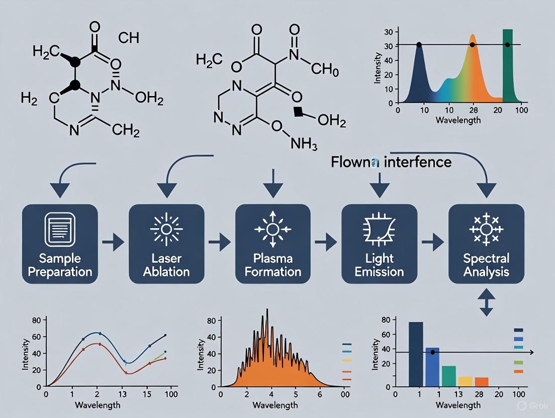
Laser-Induced Breakdown Spectroscopy (LIBS), also known as Laser Spark Spectroscopy, is an analytical technique that uses a high-powered laser pulse to analyze the elemental composition of materials [14] [15]. In LIBS imaging, this technique is extended by sweeping the laser across a sample surface in a whisk broom pattern to create detailed, spatially-resolved elemental maps [16]. The fundamental process involves several key stages:
- Laser Ablation: A short, high-intensity laser pulse (typically nanoseconds in duration) is focused onto a small spot on the sample surface [17].
- Plasma Formation: When the laser irradiance exceeds the material's ablation threshold (typically > MW/cm²), it vaporizes a minute amount of material (nanograms to micrograms) and creates a hot, ionized gas known as plasma [14].
- Spectral Emission: Atoms and ions within the plasma become excited and emit characteristic light as they decay to lower energy states [14].
- Spectral Analysis: The emitted light is collected and spectrally resolved to identify elemental composition based on unique emission line wavelengths and intensities [14].
Table 1: Key Characteristics of LIBS Imaging Technology
| Parameter | Typical Range/Value | Description |
|---|---|---|
| Laser Pulse Energy | Tens of millijoules [17] | Sufficient to generate plasma breakdown |
| Spatial Resolution | Up to 10 μm [18] | Determines smallest detectable feature |
| Sensitivity | ppm range for many elements [16] | Minimum detectable concentration |
| Ablated Mass | ng to μg per pulse [14] | Minimal sample destruction |
| Spectral Range | 200-850 nm [19] | Covers most elemental emission lines |
What are the key temporal stages of LIBS plasma evolution?
Understanding the time-resolved evolution of LIBS plasma is crucial for optimal signal detection. The plasma is a highly dynamic system that undergoes rapid changes in composition and emission characteristics [8] [17]:
Figure 1: Temporal Evolution of LIBS Plasma Emission. The diagram illustrates the sequence of emission types following laser ablation, highlighting the critical time windows for detecting different spectral features.
The optimal detection window typically begins after approximately 1 microsecond, once the continuous background radiation has sufficiently decayed to reveal discrete ionic and atomic emission lines [17]. Using time-gated detectors with delay times of 0.5-1 μs and gate widths of several microseconds is essential for suppressing continuum radiation and improving signal-to-noise ratio [8] [19].
Essential Experimental Setup and Reagents
What equipment is essential for a LIBS imaging setup?
A standard LIBS imaging system requires several core components that work together to generate, collect, and analyze plasma emission [17]:
Table 2: Essential LIBS Imaging System Components
| Component | Function | Typical Specifications |
|---|---|---|
| Pulsed Laser | Generates plasma via ablation | Nd:YAG (1064 nm), 10 ns pulse width, 10 Hz rep rate, 30 mJ energy [19] |
| Spectrometer | Disperses plasma light by wavelength | Echelle type: 200-850 nm range, 0.05 nm resolution [19] |
| Gated Detector | Time-resolved light detection | ICCD or gated CCD; gate width: ~7 μs, delay: ~0.5 μs [19] |
| Focusing Optics | Delivers laser to sample & collects emission | f/1 lens for maximum light collection [17] |
| Translation Stage | Moves sample for imaging | Precision XYZ control for micrometric resolution [18] |
| Delay Generator | Synchronizes laser & detector | Digital pulse control for precise timing [19] |
What are the critical considerations for laser selection in LIBS?
Laser parameters significantly influence plasma characteristics and analytical performance [14] [2]:
- Pulse Duration: Nanosecond lasers are most common, but femtosecond lasers offer more controlled ablation with less thermal effects [2].
- Wavelength: Fundamental Nd:YAG wavelength (1064 nm) is widely used, but harmonic wavelengths (532 nm, 355 nm) can improve coupling with certain materials [19].
- Beam Quality: Gaussian profile enables tight focusing and lower energy requirements for plasma generation [17].
- Repetition Rate: Ranges from single shot to kHz; higher rates enable faster imaging but require careful thermal management [14].
Advanced Methodologies and Data Analysis
How is hyperspectral LIBS data structured and analyzed?
LIBS imaging generates complex, three-dimensional hyperspectral datasets that require specialized analysis approaches [18]. The data structure consists of:
- Spatial Dimensions (x, y): Representing the physical coordinates of each ablation point on the sample surface.
- Spectral Dimension (λ): Containing the full emission spectrum at each spatial location.
For large hyperspectral images (potentially exceeding megapixels with thousands of spectral channels), multivariate analysis techniques like Principal Component Analysis (PCA) are essential for reducing dimensionality and extracting chemically relevant information [18]. This approach helps identify mineral phases, assess measurement quality, and isolate elemental distributions without requiring prior knowledge of all spectral lines.
What methodologies exist for combining LIBS with other techniques?
Multimodal approaches that combine LIBS with complementary techniques can significantly enhance analytical capabilities [16]. Two primary strategies have emerged:
Figure 2: Multimodal Data Analysis Strategies. Two approaches for combining LIBS with Hyperspectral Imaging (HSI): Sensor Fusion merges features from both techniques, while Knowledge Distillation uses LIBS to train HSI models.
These collaborative approaches have demonstrated remarkable success in applications such as geographical origin identification of rice, where combined LIBS-HSI with machine learning achieved 99.85% classification accuracy compared to 93.06% for LIBS alone and 88.07% for HSI alone [19].
Troubleshooting Common Experimental Issues
How can researchers diagnose and address spectral interference?
Spectral misidentification represents one of the most common errors in LIBS analysis [8]. The following systematic approach ensures accurate elemental identification:
- Multi-Line Verification: Never assign element identity based on a single emission line. Exploit the multiplicity of information from different emission lines of each element [8].
- Spectral Database Reference: Consult comprehensive atomic databases to verify all expected lines for a suspected element are present with correct relative intensities.
- Matrix-Matched Standards: Use standards with similar composition to unknown samples to account for matrix effects that can shift line positions or intensities [2].
- Wavelength Calibration: Regularly verify spectrometer calibration using known reference materials to prevent systematic shifts that cause misidentification.
Table 3: Common Spectral Interferences and Solutions
| Problem | Symptoms | Solution Approaches |
|---|---|---|
| Spectral Misidentification | Element detected that is inconsistent with sample matrix | Use multiple emission lines for confirmation [8] |
| Matrix Effects | Same element gives different signals in different materials | Use matrix-matched standards; apply calibration-free LIBS [2] |
| Self-Absorption | Calibration curves saturate at high concentrations; line centers dip | Use lines with lower transition probabilities; apply self-absorption correction algorithms [8] |
| Plasma Instability | High pulse-to-pulse signal variation | Control experimental parameters precisely; use higher laser quality [2] |
What are the common pitfalls in quantitative LIBS analysis?
Achieving reliable quantification requires understanding several analytical challenges [8] [2]:
- Distinguishing Detection from Quantification: The Limit of Detection (LOD = 3σ/b, where σ is blank standard deviation and b is calibration slope) represents the minimum detectable amount, but the Limit of Quantification (LOQ = 3-4 × LOD) is typically required for reliable measurement [8].
- Calibration Design: Use numerous standards (>10) with concentrations spanning expected ranges, including points near the expected LOQ. Avoid using only high-concentration standards [8].
- Plasma Condition Monitoring: Ensure Local Thermal Equilibrium (LTE) conditions by verifying McWhirter criterion and using time-resolved spectroscopy with gate times <1 μs for accurate temperature and electron density measurements [8].
- Chemometric Validation: When using machine learning algorithms (PLS-DA, SVM, ELM), compare results with classical univariate methods, use sufficient samples for statistical significance, and validate on external data not used for training [8] [19].
Frequently Asked Questions
How does LIBS compare to other elemental analysis techniques?
LIBS offers unique advantages and limitations compared to alternative techniques [14]:
- Versus XRF: LIBS can analyze light elements (Z < 20) that XRF cannot detect, and works equally well on conducting and non-conducting samples without requiring specialized preparation [14].
- Versus ICP-OES: While ICP-OES generally offers better relative LODs, LIBS analyzes sub-microgram quantities directly in solid samples without digestion. LIBS absolute sensitivity can be comparable when considering actual mass analyzed [2].
- Unique LIBS Advantages: Minimal sample preparation, suitability for in-situ and remote analysis, capacity to analyze any material state (solid, liquid, gas), and capacity for rapid elemental imaging [14].
What strategies can enhance LIBS sensitivity and reproducibility?
Several advanced approaches can improve LIBS performance [2]:
- Double-Pulse LIBS: Using two sequential laser pulses (collinear or orthogonal geometry) can enhance signals by up to two orders of magnitude. The first pulse creates a favorable low-density environment through shock wave expansion, while the second pulse generates more efficient plasma [8].
- Nanoparticle-Enhanced LIBS (NELIBS): Depositing nanoparticles on the sample surface can significantly improve signal intensity through enhanced laser-matter interaction and more efficient plasma formation [2].
- Advanced Signal Processing: Combining LIBS with machine learning algorithms like Light Gradient Boosting Machine (LGBM), Partial Least Squares Regression (PLSR), and Recursive Feature Elimination (RFE) can extract more information from spectra and improve quantitative accuracy [20].
- Environmental Control: Using custom chambers or controlled atmospheres (e.g., Argon instead of air) can improve hit efficiency and spectral reproducibility by minimizing atmospheric effects [20].
What are the current limitations and future directions for LIBS imaging?
While LIBS has developed significantly in recent years, several challenges remain active research areas [2]:
- Fundamental Understanding: Better first-principles prediction of plasma emission spectra from arbitrary analytes in different matrices is still needed [2].
- Instrument Reproducibility: Unlike FT-IR or UV-Vis, LIBS spectra from different instruments using the same parameters aren't necessarily identical, requiring work on standardization [2].
- Nanoscale Resolution: Extending LIBS to nanoscale imaging while maintaining sufficient signal from limited ablated mass presents significant technical challenges [2].
- Data Interpretation Expertise: The complexity of LIBS datasets (high dynamic range, spectral complexity, large data volumes) requires development of more accessible analysis tools and methodologies [18].
The field continues to evolve with promising developments in instrumentation miniaturization, improved laser technologies (diode-pumped, fiber lasers), advanced data analysis algorithms, and standardized methodologies that will further establish LIBS as a powerful analytical technique for diverse applications from planetary exploration to pharmaceutical development [14] [2].
FAQs: Core Concepts and Challenges
Q1: What are the most common types of spectral interference encountered in biomedical LIBS analysis?
The most prevalent spectral interferences in biomedical LIBS stem from the complex organic and inorganic matrix of the samples. Key scenarios include:
- Spectral Line Overlap: This occurs when emission lines from different elements are too close to be resolved by the spectrometer. In tissues and blood plasma, this is common among trace metals like iron (Fe), calcium (Ca), and sodium (Na), which have rich and dense emission spectra [1].
- Matrix Effects: Variations in the physical (e.g., density, hardness, thermal conductivity) and chemical properties of the sample can alter the laser-sample interaction, leading to changes in ablation efficiency and plasma properties. This causes signal fluctuation even when the actual elemental concentration is unchanged [6] [21]. Calcified tissues like bone and teeth are particularly susceptible due to their heterogeneous composition of hard mineral (hydroxyapatite) and soft organic components [6].
- Biomedical Sample Heterogeneity: The inherent non-uniformity of biological tissues—comprising cells, extracellular matrix, fluids, and in some cases, mineral deposits—means that sequential laser pulses may ablate materials with different compositions, leading to significant signal uncertainty [6] [22].
Q2: Why are calcified tissues like bone and teeth particularly challenging for LIBS analysis?
Calcified tissues present a "double challenge" due to their complex composite nature [6]:
- Extreme Matrix Contrast: They consist of a hard, inorganic phase (hydroxyapatite crystals) and a soft, organic phase (collagen fibers). These components have vastly different ablation thresholds and thermal properties. A single laser pulse can interact with both phases unpredictably, causing large variations in the amount and composition of ablated material [6].
- Molecular Decomposition: The high temperature of the laser plasma can cause the decomposition of hydroxyapatite, altering the observed elemental ratios. Furthermore, the analysis is often focused on detecting toxic metals or metabolic markers that are incorporated into the hydroxyapatite lattice at trace levels, making their accurate quantification difficult [6].
Q3: What methodologies can diagnose spectral interference in LIBS imaging data?
Beyond visual inspection of the mean spectrum, chemometric tools are essential for robust diagnosis:
- Principal Component Analysis (PCA): When applied to a restricted spectral range around the emission line of a specific element, PCA can reveal the presence of spectral interference. If multiple principal components explain a significant amount of variance within this narrow window, it indicates that the signal is influenced by more than one source—that is, the target element's line is interfered with [1].
- Multivariate Curve Resolution - Alternating Least Squares (MCR-ALS): Following a positive diagnosis from PCA, MCR-ALS can be used to mathematically "unmix" the complex signal into the pure contribution of the target element and the interfering species. This generates a corrected, less biased elemental distribution image [1].
Troubleshooting Guides
Scenario 1: Inaccurate Elemental Maps in Heterogeneous Tissue
Problem: Generated elemental distribution maps for trace metals (e.g., Zinc) in a breast tissue sample show suspicious correlations with major elements (e.g., Carbon), suggesting potential interference from the organic matrix or another unknown element [6] [1].
Diagnosis and Solution Workflow:
Experimental Protocol:
- Data Acquisition: Acquire LIBS hyperspectral imaging data from the tissue section. Ensure a sufficient number of spectra (>10,000) are collected to represent the tissue heterogeneity [1].
- Preliminary Mapping: Generate an initial map by integrating the signal around the primary emission line of the element of interest (e.g., Zn I 334.5 nm).
- Interference Diagnosis (PCA): Extract all spectra from the dataset. Perform PCA focusing only on a narrow spectral range (e.g., ±0.1 nm) centered on the Zn I 334.5 nm line. If the first two principal components explain a significant portion of the variance and their loadings show different spectral features, this confirms spectral interference [1].
- Interference Correction (MCR-ALS): Apply the MCR-ALS algorithm to the same narrow spectral window. The algorithm will iteratively resolve the mixed signals into pure spectral profiles and their corresponding concentration maps. Use the resolved profile that matches the known signature of your target element to generate the corrected distribution map [1].
Scenario 2: Signal Instability in Calcified Tissue (Bone) Analysis
Problem: Analysis of a bone sample for trace lead (Pb) content shows high signal fluctuation (poor RSD) from shot-to-shot, making quantification unreliable. This is driven by the matrix effect from the heterogeneous bone structure [6] [21].
Diagnosis and Solution Workflow:
Experimental Protocol:
- Morphological Analysis: Integrate a microscope with an industrial CCD camera into your LIBS system. After LIBS analysis, use a depth-from-focus imaging technique to perform 3D reconstruction of the ablation craters. Precisely calculate the ablation volume for each measurement point [21].
- Data Correlation: Perform multivariate regression analysis to investigate the correlation between the calculated ablation volume, key plasma parameters (e.g., temperature, electron density), and the intensity of the target elemental line (e.g., Pb I 405.78 nm) [21].
- Model Building: Construct a dominant factor-driven machine learning model (e.g., based on PLSR or Kernel Extreme Learning Machine). Use the ablation volume and plasma parameters as input variables to predict the corrected elemental concentration. This model actively compensates for the matrix effect [22] [21].
- Validation: Validate the model using certified reference materials or samples with known concentrations analyzed by a reference method like ICP-MS.
Essential Data Tables
Table 1: Common Spectral Interferences in Biomedical LIBS
| Element of Interest | Primary Analytical Line (nm) | Common Interfering Elements/Species | Typical Sample Type |
|---|---|---|---|
| Calcium (Ca) | 393.366 (Ca II) | Iron (Fe), Chromium (Cr) [1] | Bone, Teeth, Blood Plasma |
| Sodium (Na) | 588.995 (Na I) | Background continuum, molecular bands | Soft Tissues, Blood Plasma |
| Iron (Fe) | 248.28 (Fe I) | Matrix elements (Carbon, Calcium) [22] | Liver Tissue, Blood |
| Zinc (Zn) | 334.5 (Zn I) | Carbon (C) bands, other trace metals | Prostate Tissue, Bone |
| Lead (Pb) | 405.78 (Pb I) | Organic matrix, Calcium | Teeth, Bone |
Table 2: Performance Comparison of Interference Correction Methods
| Method | Principle | Advantages | Limitations | Best For |
|---|---|---|---|---|
| Classic Integration [1] | Signal sum over fixed window | Fast, simple, intuitive | Highly biased by interference | Quick screening of non-overlapping lines |
| MCR-ALS [1] | Spectral unmixing via chemometrics | Corrects interference, less biased maps | Requires initial diagnosis, more complex | Hyperspectral imaging of tissues |
| Dominant Factor ML [22] | ML model using ablation/plasma features | Actively corrects matrix effects, high accuracy | Requires extensive data for training | Quantitative analysis of calcified tissues |
| Internal Standardization | Normalization to a reference element | Improves precision | Difficult to find suitable internal standard | Homogeneous fluid samples (e.g., serum) |
The Scientist's Toolkit
Research Reagent Solutions for Biomedical LIBS
| Reagent / Material | Function in Experiment | Application Context |
|---|---|---|
| Certified Reference Materials (CRMs) [23] | Calibration and validation of analytical methods; provides known concentration values for quality control. | Essential for all quantitative work, especially for trace metals in serum or tissue. |
| SPADNS & DTAB Complexation Kit [23] | Preparation of multielement calibration materials by forming immobilized metal complexes on a solid substrate (e.g., photographic paper). | Creating custom, matrix-matched calibration standards for liquid samples like blood plasma or digested tissues. |
| Powdered Hydroxyapatite | Simulating the mineral phase of calcified tissues for method development and calibration. | Developing and optimizing methods for bone and teeth analysis before using real clinical samples. |
| Buffered Solutions (pH 8.0) [23] | Controls the pH during complexation reactions to ensure efficient formation and adsorption of metal:SPADNS/DTAB ion pairs. | Critical for preparing the custom calibration materials using the SPADNS/DTAB method. |
FAQs on Spectral Interference in LIBS
What is spectral interference in LIBS and why is it a problem? Spectral interference occurs when the emission line of an element you are trying to measure (the analyte) overlaps with an emission line from a different element or a molecular band present in the sample. In LIBS imaging, where maps are generated by integrating the signal at a wavelength assumed to be specific to an element, any interference inevitably results in a biased distribution image. This can show over-concentrations of the element or even falsely indicate its presence in areas where it is absent [1].
What are the common root causes of spectral interference? The primary causes are intrinsically linked to the strengths of LIBS itself:
- Sample Complexity: Real-world samples, such as complex rocks, biological tissues, or industrial materials, are often composed of numerous elements. This diversity increases the probability of emission lines from different elements being close in wavelength [1] [2].
- Rich LIBS Spectra: LIBS is capable of detecting most elements in the periodic table, each of which can emit hundreds of spectral lines. This richness, combined with the low bandwidth of emission lines, makes finding a completely isolated and characteristic wavelength for an element difficult [1] [8].
- Elemental Co-localization: In heterogeneous samples, different elements can be located in the same microscopic area. When the laser ablates this area, all these elements are excited simultaneously, and their emitted light is collected from the same plasma volume, leading to superimposed spectral signals [1].
How can I diagnose if my LIBS data has spectral interference? Classically, interference is suspected when elemental maps show unexpected correlations or when known sample features do not align with the chemical map. A powerful diagnostic method uses Principal Component Analysis (PCA). By applying PCA to a restricted spectral range around your element's wavelength of interest, you can identify the presence of multiple, independent chemical sources contributing to the signal in that region. If PCA loadsings show more than one significant component in the narrow window, it is a strong indicator of spectral interference [1].
What can I do to correct for spectral interference? Once diagnosed, interference can be corrected using spectral unmixing techniques. Multivariate Curve Resolution-Alternating Least Squares (MCR-ALS) is one effective method. MCR-ALS can be applied to the restricted spectral domain to mathematically resolve the pure contribution of the element of interest from the overlapping signals, generating a less biased chemical distribution map [1].
Troubleshooting Guide: Diagnosing and Correcting Spectral Interference
This guide provides a step-by-step protocol for handling spectral interference, from initial suspicion to a corrected image.
Problem: A generated elemental map shows a suspicious distribution, likely biased by spectral interference.
Step 1: Initial Qualitative Check
- Action: Compare your elemental map to the distribution of other major elements in the sample.
- Interpretation: If the map of your element of interest (e.g., Silicon) appears unusually similar to the map of another element (e.g., Carbon), this unexpected correlation is a red flag for potential spectral interference [1].
Step 2: Confirm with Principal Component Analysis (PCA)
- Objective: Diagnose the presence of multiple chemical components in the spectral range of interest.
- Protocol:
- Isolate Spectral Window: Do not use the full spectrum. Extract a narrow spectral range centered on the analyte's emission line (e.g., Si I 288.158 nm).
- Perform PCA: Apply PCA to this restricted hyperspectral cube.
- Analyze Loadings: Examine the PCA loadings. The presence of more than one significant component in this narrow window indicates that the signal is not pure and that spectral interference is likely present [1].
Step 3: Correct with Multivariate Curve Resolution (MCR-ALS)
- Objective: Resolve the mixed signal into its pure components to obtain a corrected image.
- Protocol:
- Input Data: Use the same restricted spectral window as in the PCA diagnosis.
- Apply MCR-ALS: Use the MCR-ALS algorithm to decompose the data. The model is
D = CS^T + E, whereDis the original data matrix,Cis the matrix of resolved concentrations (distribution maps),S^Tis the matrix of resolved pure spectra, andEis the residual noise. - Generate Corrected Map: From the resolved concentration matrix
C, extract the component corresponding to your element of interest to produce a corrected, less biased distribution image [1].
The following workflow diagram illustrates the diagnostic and correction process:
Experimental Protocol: Interference Diagnosis via PCA
This protocol details the methodology for using PCA to diagnose spectral interference, as demonstrated on a complex rock sample [1].
1. Sample Preparation and Data Acquisition
- Sample: A polished thin section of a complex rock (e.g., germanium and gallium zoned sphalerite in a quartz and mica matrix).
- LIBS Instrument: A LIBS imaging setup, typically involving a pulsed Nd:YAG laser (e.g., 266 nm, 50 Hz, 4 mJ) and a Czerny-Turner or Echelle spectrometer.
- Acquisition Parameters: The sample surface is mapped with a spatial resolution of 10-20 μm. A hyperspectral data cube is acquired where each pixel contains a full LIBS spectrum [1] [24].
2. Data Pre-processing
- Action: Before analysis, spectra may be pre-processed. Common steps include:
- Background Subtraction: Removing the dark signal from the detector.
- Continuum Removal: Using a spline fit or moving minimum calculation to subtract the underlying continuum radiation, which helps in better peak analysis [25].
- Spectral Alignment: Correcting for any minor instrumental shift in wavelength calibration.
3. Restricted Spectral Analysis via PCA
- Action: Instead of using the full spectrum, isolate a window around the analyte line. For example, for the Silicon line at 288.158 nm, a window of ±1 nm might be used.
- Perform PCA: Apply PCA to this 3D hyperspectral block (X, Y, Wavelength).
- Diagnosis: Analyze the loadings of the first few Principal Components. If the first PC alone does not explain nearly all the variance, and the loadings of PC2 (and higher) show distinct spectral features within the window, this confirms the presence of multiple emitting species and thus, spectral interference [1].
The Scientist's Toolkit: Essential Reagents & Materials
The following table lists key materials and software tools used in the featured experiments for diagnosing and correcting spectral interference.
| Item Name | Function / Explanation |
|---|---|
| Complex Rock Sample (e.g., zoned sphalerite) | A heterogeneous sample with known elemental co-localization, used to demonstrate and validate interference scenarios [1]. |
| Polished Thin Section | Standard geological preparation that provides a flat surface for accurate LIBS imaging and prevents topographical artifacts [1]. |
| NIST Atomic Spectra Database | Critical reference database for identifying theoretical emission lines of elements and identifying potential overlaps [24] [25]. |
| Multivariate Analysis Software (e.g., MATLAB, Python with scikit-learn) | Platform for implementing chemometric tools like PCA and MCR-ALS, which are central to the diagnostic and correction workflow [1] [25]. |
| Comb Filter Algorithm | A novel software tool that uses "comb" templates of elemental spectral fingerprints to autonomously detect elements and identify regions of spectral interference [24]. |
Advanced Diagnostic Techniques: PCA, MCR-ALS and Machine Learning for Interference Detection
Laser-Induced Breakdown Spectroscopy (LIBS) is a rapid, laser-based analytical technique used for the elemental analysis of various materials. The core principle involves using a high-power laser pulse to create a micro-plasma on the sample surface; as this plasma cools, excited atoms and ions emit light at characteristic wavelengths, creating a unique spectral fingerprint for the sample's composition [26] [27]. In LIBS imaging, where multiple spectra are collected across a sample surface to create elemental maps, dealing with the full, complex spectrum can be computationally intensive and may dilute the signal from key analytes. Restricted Spectral Range Analysis (RSRA) is a chemometric strategy that enhances analytical precision and diagnostic power by focusing computational efforts on pre-selected, diagnostically rich Regions of Interest (ROIs) within the electromagnetic spectrum. This approach is particularly vital for diagnosing and mitigating spectral interference in LIBS imaging research, as it allows researchers to isolate the signals of target elements from a complex background, leading to more accurate and reliable quantitative and qualitative results.
Core Concepts and FAQs
This section addresses fundamental questions about the principles and application of Restricted Spectral Range Analysis.
FAQ 1: What is Restricted Spectral Range Analysis, and why is it crucial for diagnosing spectral interference in LIBS?
Spectral interference occurs when the emission lines of different elements overlap within a LIBS spectrum, leading to misidentification or inaccurate quantification [8]. Restricted Spectral Range Analysis is a targeted methodology where subsequent chemometric processing is confined to specific, limited wavelength regions that contain the most analytically useful information for a given application. This is crucial for diagnosing interference because it:
- Isolves Analytic Signals: It allows researchers to focus on the specific spectral lines of target elements, making it easier to identify and diagnose overlapping lines from interferents.
- Reduces Complexity: By ignoring spectrally "barren" regions, it simplifies the data matrix, which can improve the performance and stability of multivariate calibration models.
- Enhances Sensitivity: Concentrating on a narrow ROI can improve the signal-to-noise ratio for trace elements, whose subtle, "peak-free" signatures might otherwise be lost in the full-spectrum background [28].
FAQ 2: How does focusing on a Region of Interest (ROI) improve a LIBS-based calibration model?
Focusing on an ROI provides several key advantages that translate directly into a more robust calibration model:
- Mitigates the "Curse of Dimensionality: A full LIBS spectrum can contain thousands of data points. Many of these are irrelevant to the specific analyte and act as noise, which can degrade model performance. RSRA reduces the number of variables, leading to a more parsimonious and reliable model.
- Minimizes Matrix Effects: The LIBS signal is notoriously affected by the sample matrix, where the presence of other elements can influence the emission intensity of the analyte [2]. By strategically selecting an ROI less prone to known spectral overlaps from the matrix, the model's accuracy and transferability across different sample types can be improved.
- Increases Model Interpretability: A model built on a limited set of known, relevant emission lines is far easier to interpret and validate physically than a "black box" model using the entire spectrum.
Troubleshooting Guides
Guide: Diagnosing and Resolving Spectral Interference in a Selected ROI
Spectral interference is a primary challenge in quantitative LIBS. This guide outlines a systematic approach to diagnose and correct for it within a chosen ROI.
Problem: A calibration model for a target element in a specific ROI is performing poorly, suspected to be due to spectral interference from the sample matrix.
Step-by-Step Diagnostic Protocol:
- Verify Peak Assignment: Misidentification of spectral lines is a common error [8]. Cross-reference all peaks in your ROI against a standard database (e.g., NIST). Never base identification on a single emission line; confirm using multiple lines for the same element [8].
- Spike the Sample: If possible, introduce a known concentration of the target analyte into the sample. If the corresponding peak in the ROI increases proportionally without altering the shape of other peaks, interference is less likely. If the peak shape changes or other peaks are affected, it suggests overlap.
- Analyze a Pure Interferent: Collect a LIBS spectrum from a sample containing a high-purity version of the suspected interfering element. Compare its spectrum to your ROI to confirm the presence and intensity of the overlapping line.
- Employ Advanced Algorithms: Use spectral fitting or deconvolution algorithms, such as the Boosted Deconvolution Fitting (BDF) method, which can resolve overlapping bands even when their separation is smaller than the classical Sparrow's resolution criterion [29].
Resolution Strategies:
- ROI Refinement: If interference is confirmed, narrow the ROI further to exclude the most affected portion of the spectrum, or shift to a secondary, less intense emission line for the target analyte that is free from overlap.
- Multivariate Correction: Instead of using a single peak (univariate analysis), employ multivariate methods like Partial Least Squares Regression (PLSR). PLSR can leverage the entire shape of the spectral interference within the ROI to deconvolute the contributions of the target and interferent [30].
- Machine Learning: Implement a back-propagation neural network or similar machine learning model. These are highly effective at learning the complex, non-linear relationships caused by interference and correcting for spectral intensity variations [31].
Table 1: Common Spectral Interferences and Potential Resolution Strategies.
| Target Element (Line) | Common Interferent (Line) | Diagnostic Method | Resolution Strategy |
|---|---|---|---|
| Cadmium (Cd I 226.5 nm) | Calcium (Ca II 226.4 nm) | Analyze pure Ca sample; check for secondary Cd lines | Switch to Cd I 214.4 nm line; use PLSR |
| Phosphorus (P I 213.6 nm) | Copper (Cu I 213.6 nm) | Spike sample with P; observe peak shape | Use multivariate analysis (PLSR) on a wider ROI |
| Silicon (Si I 288.16 nm) | Iron (Fe I 288.07 nm) | Consult NIST database; use high-resolution spectrometer | Apply a deconvolution algorithm (e.g., BDF) [29] |
Guide: Selecting an Optimal Region of Interest for Your Application
Choosing the correct ROI is a critical step that dictates the success of the entire RSRA workflow.
Objective: To define a spectral region that maximizes the signal for your target analyte(s) while minimizing background and interference.
Selection Workflow:
- Define Analytical Goals: Clearly state whether the goal is quantitative analysis of a specific element, qualitative discrimination between sample classes, or detection of trace biomarkers.
- Initial Spectral Survey: Collect high-quality, representative LIBS spectra from all sample types of interest (e.g., healthy vs. diseased tissue, different alloy grades).
- Identify Candidate Lines: For quantitative work, select the most intense, well-resolved emission lines for your target elements. For fingerprinting or classification, identify regions that show the greatest variance between classes. Trace biometal analysis in blood, for instance, may focus on subtle, "peak-free" regions where chemometrics can extract diagnostic patterns [28].
- Check for Overlap: Use spectral databases and experimental data from pure materials to assess potential overlaps in the candidate regions.
- Validate ROI Performance: Test the selected ROI by building a preliminary calibration or classification model and evaluating its figures of merit (e.g., accuracy, precision, limit of detection).
Table 2: Example Regions of Interest for Different Application Fields.
| Application Field | Target Analytes | Suggested ROI (Example) | Rationale |
|---|---|---|---|
| Biomedical Diagnostics (Malaria) [28] | Cu, Zn, Fe, Mg | 320-330 nm, 490-510 nm | Regions with key lines for trace biometals that act as disease biomarkers. |
| Metallurgy (Aluminum Alloys) [31] | Mg I, Mg II | 279-286 nm | Contains strong atomic (Mg I 285.2 nm) and ionic (Mg II 280.3 nm) lines for a minor element, allowing study of plasma conditions. |
| Environmental Soils [27] | K, Ca, Na, Li | 650-850 nm | Region for lighter alkali and alkaline earth metals, useful for soil fingerprinting and classification. |
The following workflow diagram summarizes the key steps for selecting and validating a Region of Interest.
Experimental Protocols
Protocol: Building a Quantitative Model Using a Restricted Spectral Range
This protocol details the steps for creating a robust quantitative calibration model for a minor element (e.g., Magnesium in aluminum alloys) using an ROI, based on a published experimental approach [31].
1. Sample and Instrument Preparation:
- Samples: Use a set of certified reference materials (e.g., eight certified aluminum alloy samples with a gradient of Mg concentration from 23 to 1360 ppm).
- Laser: A Q-switched Nd:YAG laser (1064 nm, 10 Hz). The laser pulse energy should be monitored and can be varied (e.g., from 7.9 to 71.1 mJ) to test model robustness.
- Spectrometer: An echelle spectrometer with an ICCD camera is ideal for broad, simultaneous coverage. Set the acquisition parameters (e.g., delay: 1000 ns, gate: 2000 ns) to ensure plasma is in Local Thermal Equilibrium (LTE) [31] [8].
- Sampling: Perform multiple replicates (e.g., 20) per sample, with each spectrum being an accumulation of multiple shots (e.g., 100) from fresh sample spots to account for shot-to-shot variation [30].
2. Data Acquisition and ROI Selection:
- Collect all spectra from the standard and unknown samples.
- Based on the initial survey, select an ROI that contains strong, characteristic lines for the analyte with minimal known interference. For Mg, a suitable ROI is 279-286 nm, which contains the Mg II 280.3 nm and Mg I 285.2 nm lines [31].
3. Data Pre-processing and Model Building:
- Extract ROI: From every full spectrum, extract only the data points within the selected ROI.
- Pre-process: Apply standard pre-processing to the ROI data. Common steps include:
- Normalization: Correct for pulse-to-pulse energy variation. Standard normalizations include Total Spectral Intensity (within the ROI) or Internal Standard normalization (using a matrix element line).
- Averaging: Average the replicate spectra for each sample.
- Machine Learning Correction: For higher precision, a machine learning model (e.g., neural network) can be trained to correct for intensity fluctuations due to laser energy changes [31].
- Build Model: Use the pre-processed ROI data to build a calibration model.
- Univariate: Plot the intensity of a single Mg line against concentration.
- Multivariate (Recommended): Use Partial Least Squares Regression (PLSR) on the entire ROI to create a more robust model that accounts for residual background and subtle matrix effects [30].
4. Model Validation:
- Use cross-validation or an independent test set of certified standards to validate the model's accuracy and precision. The model built using the ROI and multivariate correction should achieve a high precision (e.g., ~6.3% RSD for Mg in Al alloys) [31].
Protocol: "Peak-Free" Chemometric Analysis for Disease Diagnostics
This protocol describes a method for using RSRA and chemometrics to analyze trace biometals in blood for disease diagnosis (e.g., malaria), even when the elemental signatures are too subtle to form distinct peaks ("peak-free" LIBS) [28].
1. Sample Preparation:
- Collect peripheral finger blood drops (e.g., from healthy volunteers and Plasmodium falciparum-infected patients) with ethical approval.
- Directly dry spot the blood (~6 µL) onto clean Nucleopore membrane filters. This creates a stable, solid-phase sample for LIBS analysis with minimal preparation [28].
2. LIBS Spectral Acquisition:
- Use a hand-held or portable LIBS system for clinical feasibility.
- Acquire spectra from multiple spots on each dried blood spot to account for heterogeneity. Accumulate shots to improve the signal-to-noise ratio.
3. Restricted Spectral Range and Chemometric Analysis:
- ROI Selection: Do not focus on prominent, isolated peaks. Instead, select broad ROIs (e.g., spanning tens of nanometers) where the trace biometals (Cu, Zn, Fe, Mg) are known to have multiple, albeit weak, emission lines. The diagnostic information is contained in the subtle, multivariate pattern of these "peak-free" regions.
- Data Processing Workflow:
- Feature Selection: Use a standard sample to delineate the specific spectral regions (sub-ROIs) most associated with the target biometals.
- Principal Component Analysis (PCA): Perform PCA on the data from the selected ROIs. This reduces the dimensionality of the data and transforms the subtle spectral variations into a new set of variables (Principal Components) that best differentiate the sample classes.
- Artificial Neural Network (ANN) Modeling: Feed the scores from the significant Principal Components into an Artificial Neural Network. The ANN is trained to classify the samples (e.g., infected vs. healthy) or even predict the level of infection (parasitemia) based on the altered levels and complex correlations of the trace biometals [28].
The following diagram illustrates this "peak-free" analytical workflow.
The Scientist's Toolkit: Research Reagent Solutions
Table 3: Essential Materials and Computational Tools for RSRA in LIBS.
| Item Name | Function / Utility | Example / Specification |
|---|---|---|
| Certified Reference Materials (CRMs) | Essential for quantitative model calibration and validation. Provides known concentrations for building reliable models. | Certified aluminum alloys [31]; synthetic glass standards; pure metal samples for interference checks. |
| Nucleopore Membrane Filters | An ideal substrate for preparing homogeneous solid samples from liquids like blood or soil suspensions. Minimizes sample preparation. | Used for drying blood spots in biomedical LIBS studies [28]. |
| Echelle Spectrometer | A type of spectrometer that provides a very broad spectral range in a single shot without scanning, crucial for effective ROI selection. | Andor Mechelle 5000 [31]. |
| Q-Switched Nd:YAG Laser | The most common laser source for LIBS. Provides high-power, short pulses necessary for plasma formation. | Fundamental wavelength: 1064 nm; harmonics: 266 nm, 213 nm [30]. |
| Boosted Deconvolution Fitting (BDF) Algorithm | An advanced spectral analysis method that enhances resolution and accurately fits overlapping bands, superior to traditional methods like LMA in some cases [29]. | Resolves bands with separations smaller than Sparrow's criterion; implemented in MATLAB [29]. |
| Partial Least Squares Regression (PLSR) | A core multivariate chemometric tool for building quantitative calibration models from complex spectral data in an ROI. | Used for quantitative analysis and material discrimination [30]. |
| Artificial Neural Network (ANN) | A powerful machine learning algorithm for non-linear calibration and complex classification tasks, such as diagnosing disease from subtle spectral patterns [28]. | Used for classifying malaria-infected blood samples based on trace biometal patterns [28]. |
Frequently Asked Questions (FAQs)
Q1: What is spectral interference in LIBS, and why is it a problem for my analysis?
Spectral interference occurs when emission lines from different elements overlap within the LIBS spectrum. This overlap can lead to incorrect element identification, inaccurate quantification, and misrepresentation of elemental distributions in imaging studies. In complex samples like minerals or biological tissues, interferences are common due to the dense spectral lines of elements like iron (Fe), titanium (Ti), or calcium (Ca) [32]. These interferences hinder reliable automated line identification and can produce false positives or negatives in your results [32].
Q2: How can PCA help in diagnosing spectral interference?
PCA is a multivariate statistical technique that reduces the dimensionality of complex LIBS datasets. It transforms the original spectral variables (intensities at specific wavelengths) into a new set of variables called Principal Components (PCs). When spectral interference exists, PCA can reveal hidden patterns and correlations between different emission lines. For instance, if two wavelengths consistently vary together across many spectra, it may suggest they originate from the same mineral phase or element. Conversely, unusual behavior in a PC score plot can highlight spectra where interference is occurring, allowing you to identify and isolate these problematic measurements for further investigation [33].
Q3: My LIBS data is very large. Can PCA still be applied effectively?
Yes. PCA is particularly well-suited for handling the large, high-dimensional datasets generated by LIBS imaging, which can comprise thousands or even hundreds of thousands of spectra [32]. The computational process involves calculating the eigenvectors of the covariance matrix of your data. While this can be computationally intensive, many modern software packages (like AtomAnalyzer) have built-in PCA nodes optimized for such tasks [34]. It is often practical to begin your analysis on a representative subset of your data to establish the optimal parameters before processing the entire dataset.
Q4: What are the main limitations of using PCA for interference diagnosis?
While powerful, PCA has limitations. Its outcomes are highly dependent on proper data pre-processing (e.g., normalization, baseline correction) [35]. The principal components themselves can sometimes be difficult to interpret physically, as they represent mathematical combinations of original spectral features. PCA is an unsupervised technique, meaning it identifies patterns without prior knowledge; while this is useful for exploration, it does not directly confirm the identity of interfering elements. Finally, its effectiveness can diminish with very low signal-to-noise ratios, where weak interference patterns may be obscured [33].
Q2: I've run PCA and found outliers. How do I know if they are due to spectral interference or just random noise?
Distinguishing interference from noise requires a systematic approach. First, examine the loadings of the principal components that characterize the outliers. Loadings show which original wavelengths contribute most strongly to that PC. If the loadings plot shows two or more known emission lines from different elements with significant and similar weights, this is strong evidence of potential interference [32]. Second, you can cross-reference these suspect wavelengths against atomic databases (like NIST) to check for known overlaps. Finally, inspect the individual outlier spectra visually; true interference often presents as asymmetrical or abnormally broadened peaks compared to clean lines in other spectra.
Troubleshooting Guides
Issue 1: Poor Separation in PCA Scores Plot
Problem: After running PCA, the scores plot (e.g., PC1 vs. PC2) shows a single, tight cluster with no clear separation between different sample classes or regions.
| Possible Cause | Diagnostic Steps | Solution |
|---|---|---|
| Insufficient Signal-to-Noise Ratio | Calculate the average signal-to-noise ratio (SNR) of your spectra. Check if key emission lines are distinguishable from the background. | Increase the number of laser pulses per spot; use higher laser energy (if applicable); ensure optimal detector gate settings [6]. |
| Inadequate Pre-processing | Verify the steps in your pre-processing workflow. Plot spectra before and after processing to check for artifacts. | Apply appropriate normalization (e.g., vector, internal standard) to minimize pulse-to-pulse variation. Ensure robust baseline correction is performed [35]. |
| Selected Spectral Range is Uninformative | Check the loadings of the first few PCs. If loadings are flat, the chosen range may lack characteristic elemental lines. | Re-run PCA on a wider spectral range or on specific sub-regions known to contain diagnostic lines for the elements of interest [33]. |
Issue 2: Uninterpretable PCA Loadings
Problem: The loadings plots appear noisy and do not show clear, distinct peaks, making it impossible to link Principal Components to specific elements or interferences.
| Possible Cause | Diagnostic Steps | Solution |
|---|---|---|
| High Degree of Shot-to-Shot Fluctuation | Calculate the relative standard deviation (RSD) of intensities for a major element line across single-shot spectra. | Use ensemble averaging of multiple spectra (e.g., 10-100 shots) per spatial location to improve stability before PCA [33]. |
| Widespread Spectral Interferences | Manually inspect averaged spectra from different regions for peak asymmetry and unusual broadening. | Employ more advanced algorithms like ALIAS (Automated Line Identification for Atomic Spectroscopy) specifically designed to deconvolve interferences in complex spectra [32]. |
| Incorrect Normalization | Check if the normalization method (e.g., total intensity) is being dominated by a few, highly variable lines. | Switch to a different normalization strategy, such as using an internal standard element known to be stable across all samples [35]. |
Issue 3: PCA Fails to Identify Known Interferences
Problem: You are aware of a specific spectral interference from literature or database checks, but your PCA results do not highlight it.
| Possible Cause | Diagnostic Steps | Solution |
|---|---|---|
| The Interference is Constant | If the ratio between the interfering elements is consistent across all analysis points, PCA will not detect it as a source of variance. | Use a library of pure element spectra or synthetic spectra to perform correlation analysis or spectral angle mapping, which can flag consistent overlaps [7] [32]. |
| Low Variance from Interference | The interference may contribute very little to the overall variance in the dataset compared to other factors like major element concentration. | Apply feature selection to focus the PCA on the spectral region where the interference occurs, thereby amplifying its contribution to the variance model [35]. |
Experimental Protocols
Protocol 1: A Standard Workflow for PCA-Based Interference Diagnosis in LIBS Imaging
This protocol provides a step-by-step methodology for using PCA to uncover hidden spectral interferences.
1. Sample Preparation and Data Acquisition
- Prepare your sample according to standard procedures (e.g., pressed pellets, polished sections).
- Acquire LIBS spectral imaging data. For optimal PCA results, it is recommended to acquire a minimum of three repeated measurements (shots) per spatial location and ensure the dataset includes spectra from all expected mineral phases or tissue types [33].
2. Data Pre-processing
- Spectral Binning: If the spectral resolution is very high, bin pixels by 2-4 to reduce noise and computational load.
- Background Subtraction: Apply a baseline correction algorithm (e.g., asymmetric least squares, polynomial fitting) to remove continuum background.
- Normalization: Normalize each spectrum to its total intensity (area under the curve) or to an internal standard element to minimize signal fluctuation effects. Critical Step: The choice of normalization can dramatically affect PCA results [35].
3. Data Assembly and PCA Calculation
- Assemble all pre-processed single-shot or averaged spectra into a single data matrix ( D ) of dimensions ( m \times n ), where ( m ) is the number of spectra and ( n ) is the number of wavelength variables.
- Mean-center the data (subtract the mean spectrum from each individual spectrum).
- Input the mean-centered matrix into a PCA algorithm. This can be done using software like AtomAnalyzer [34], MATLAB, Python (scikit-learn), or R.
4. Interpretation and Interference Diagnosis
- Scores Analysis: Examine the scores plot (e.g., PC1 vs. PC2) to identify clusters, trends, and—most importantly—outliers. Spectra that are clear outliers often contain unusual phenomena, including severe spectral interferences [33].
- Loadings Analysis: For the principal components that define clusters or outliers, plot the corresponding loadings. The loadings indicate which wavelengths (and therefore which elements) are responsible for the observed variance.
- Cross-referencing: Identify peaks in the loadings plots and cross-reference the wavelengths with the NIST atomic database. Look for loadings plots where multiple known emission lines from different elements contribute significantly to the same PC, indicating a correlated variance that may stem from interference.
The following workflow diagram summarizes this diagnostic process:
Protocol 2: Validating Suspected Interferences Using the ALIAS Methodology
When PCA indicates a potential interference, the ALIAS (Automated Line Identification for Atomic Spectroscopy) methodology provides a robust framework for confirmation [32].
1. Peak Detection
- Input an averaged, high signal-to-noise spectrum from a representative region.
- Apply an automated peak detection algorithm to identify all significant emission lines in the spectrum.
2. Generation of a Synthetic Spectrum
- For a list of candidate elements (including those suspected from PCA loadings), generate a theoretical synthetic spectrum.
- This synthetic spectrum is based on a simplified plasma model and uses known transition probabilities from the NIST database to predict relative line intensities [32].
3. Similarity Analysis and Decision
- Compute similarity coefficients between the experimental spectrum and the synthetic spectra for each candidate element.
- The algorithm then assigns a probabilistic assessment for each detected peak, identifying which element it most likely belongs to and flagging peaks where multiple elements could be contributing (i.e., interference) [32].
This validation process is structured as follows:
The Scientist's Toolkit: Key Research Reagent Solutions
The following table details essential computational tools and algorithms used in advanced interference diagnosis for LIBS imaging research.
| Tool/Algorithm Name | Type | Primary Function in Interference Diagnosis |
|---|---|---|
| Principal Component Analysis (PCA) [33] [35] | Unsupervised Multivariate Algorithm | Reduces data dimensionality to reveal hidden patterns and outliers indicative of spectral interference. |
| ALIAS (Automated Line Identification for Atomic Spectroscopy) [32] | Automated Identification Algorithm | Uses synthetic spectra and similarity coefficients to reliably assign peaks to elements and flag interferences. |
| Comb-like Filter Algorithm [7] | Correlation-based Filter | Correlates element-specific "fingerprint" filters with experimental data, robust to instrumental drift. |
| AtomAnalyzer Software [34] | Commercial LIBS Software | Provides a modular workflow (including PCA nodes) for processing and visualizing LIBS data. |
| NIST Atomic Spectra Database | Reference Database | The primary reference for elemental emission lines and relative intensities, essential for identifying potential overlaps. |
Multivariate Curve Resolution-ALS (MCR-ALS) for Spectral Unmixing and Interference Correction
Frequently Asked Questions (FAQs)
Q1: What is the fundamental principle behind MCR-ALS? MCR-ALS is a "soft-modeling" algorithm that decomposes a series of multi-component spectra into two matrices: a concentration matrix (C) containing the concentration profiles of each pure component, and a spectra matrix (ST) containing their pure spectral signatures. It operates based on the bilinear model D = CST + E, where D is the original data matrix and E is the residual matrix [36] [37].
Q2: Under what conditions is MCR-ALS applicable to LIBS imaging data? The primary condition is the bilinearity of the data, meaning the total measured spectrum must be a weighted sum of the pure component spectra, with the weights corresponding to their concentrations [36]. LIBS imaging data, where each pixel's spectrum is a mixture of emissions from different elemental or molecular species, generally meets this requirement.
Q3: What are the most critical constraints applied during MCR-ALS and why? The most common and critical constraints are:
- Non-negativity: Forces both concentration profiles and spectral intensities to be positive, as negative values are physically meaningless in most spectroscopic contexts [38].
- Unimodality: Applied to concentration profiles when a component appears and disappears only once during a process (e.g., in kinetic studies) [36].
- Closure: Forces the sum of concentrations of all components in a sample to equal a constant, typically 1 or 100% [37].
Q4: How can I diagnose if my MCR-ALS results are reliable? Reliability can be assessed by:
- Examining the residual matrix (E): It should contain only random noise, not structured patterns.
- Checking the convergence: The algorithm should converge to a stable solution.
- Using known information: If the pure spectrum or concentration profile of one component is known, it can be fixed during the optimization to guide the model and validate the output [38].
Q5: My MCR-ALS analysis fails to converge. What could be the cause? Non-convergence can stem from:
- Incorrect number of components: Over- or under-estimating the number of components in the mixture.
- Poor initial estimates: The starting points for the iterative optimization are too far from the true solution.
- Inappropriate constraints: The applied constraints may be too restrictive or conflict with the underlying data structure.
Troubleshooting Guides
Issue 1: Poor Resolution Due to Severe Spectral Overlap
Problem: The resolved concentration profiles and spectra are mixed, inaccurate, and do not represent pure components. This is common in complex samples like geological materials or biological tissues where multiple elements emit light at similar wavelengths [36] [39].
Solution:
- Apply Tailored Constraints: Incorporate all available physical knowledge about the system as constraints. For instance, in a kinetic study, apply unimodality to the concentration profile of a transient intermediate [36].
- Matrix Augmentation: Combine data from multiple experiments or analytical techniques (e.g., LIBS and Raman) into a single data matrix. This provides more information and helps break the rotational ambiguity inherent in MCR solutions [36].
- Fix Known Profiles: If the spectrum or concentration profile of one component is known from standards or other measurements, fix it during the ALS optimization to improve the resolution of the remaining components [38].
Issue 2: Handling Non-Ideal Data (Noise and Baseline Drift)
Problem: The presence of high noise levels or significant baseline drift in LIBS spectra violates the bilinearity assumption and leads to poor unmixing performance.
Solution:
- Pre-processing: Apply spectral pre-processing before MCR-ALS.
- Smoothing: Use Savitzky-Golay filters to reduce high-frequency noise.
- Baseline Correction: Apply algorithms (e.g., asymmetric least squares) to remove background and drift.
- Leverage Spatial Information: For LIBS imaging data, use the spatial context. Techniques operating in the Fourier space can help identify spectral ranges that contain meaningful spatial information, which can then be weighted more heavily in the analysis [3].
Issue 3: Determining the Correct Number of Components
Problem: Selecting too few components fails to describe the data, while selecting too many leads to overfitting and the resolution of physically meaningless "noise components."
Solution:
- Exploratory Data Analysis: Use Principal Component Analysis (PCA) and examine the scree plot of explained variance to estimate the number of significant components.
- Core Consistency Diagnostic: A method often used in parallel factor analysis (PARAFAC) that can be adapted to evaluate the appropriateness of the model for a given number of components.
- Iterative Fitting and Validation: Run MCR-ALS with different numbers of components and validate the results physically (e.g., do the resolved spectra have realistic peak shapes?) and chemically (e.g., do the concentration profiles make sense?).
Experimental Protocols for Key Applications
Protocol 1: Resolving Interfering Elements in a Geologic Sample
This protocol is designed to resolve the complex elemental distributions in a speleothem (cave deposit) sample, where elements like Mg, Pb, and Cu may have overlapping emission lines [39].
1. Sample Preparation:
- Prepare a polished thin section of the speleothem sample.
- If available, use certified reference materials with known concentrations of the target elements for qualitative comparison.
2. LIBS Imaging Data Acquisition:
- Instrument: Use a micro-LIBS system with an Nd:YAG laser (1064 nm) and a Czerny-Turner spectrometer coupled to an ICCD camera [39].
- Parameters:
- Laser Pulse Energy: ~1 mJ
- Repetition Rate: 100 Hz
- Spot Size: ~7 µm
- Step Size: 24 µm (to avoid crater overlap)
- Atmosphere: Ambient air or argon for enhanced signal
- Output: A hyperspectral data cube
D_rawof dimensions (xpixels, ypixels, n_wavelengths).
3. Data Pre-processing:
- Background Subtraction: Remove dark noise from the ICCD camera.
- Wavelength Calibration: Use a standard lamp (e.g., Hg(Ar)) for accurate wavelength alignment.
- Baseline Correction: Apply a rolling-circle or polynomial fit algorithm to remove the continuum background from each spectrum.
- Normalization: Normalize spectra to the total intensity or an internal standard (e.g., a Calcium line) to correct for shot-to-shot signal fluctuations.
- Data Arrangement: Unravel the 2D spatial data into a single matrix
Dof size (npixels, nwavelengths).
4. MCR-ALS Analysis:
- Software: Utilize a library such as
pyMCR[38]. - Initialization: Estimate initial spectral components
ST_initialusing a simple method like Vertex Component Analysis (VCA) [40]. - Constraints:
- Apply non-negativity to both concentration (
C) and spectra (S^T) matrices. - Apply a closure constraint if the data represents relative abundances.
- Apply non-negativity to both concentration (
- Execution: Fit the model using
mcrar.fit(D, ST=ST_initial)and iterate until convergence (e.g., change in residuals < 0.1%).
5. Validation:
- Compare the resolved spectral profiles
S^Twith known NIST atomic emission databases to identify elements. - Correlate the resolved concentration maps
Cwith optical images of the sample's growth layers [39].
Protocol 2: Diagnosing and Correcting Spectral Interference in LIBS
This protocol provides a systematic workflow for diagnosing and mitigating the impact of spectral interference on MCR-ALS analysis.
1. Diagnosis of Spectral Interference:
- Inspect the Average Spectrum: Plot the mean spectrum of the entire dataset. Look for peaks that are abnormally broad or asymmetric, which suggest overlapping emission lines [39].
- Spatial Information Analysis: Calculate a spatial information ratio metric in the Fourier space for each wavelength. Wavelengths with low spatial information are likely dominated by noise or non-specific background, while those with high spatial information but broad peaks may indicate interference [3].
- Create a 2D Scatter Plot (Pixel-Vector Plot): Plot the intensity of one suspected wavelength against another. A distribution that is not a straight line from the origin suggests the presence of at least two independently varying components contributing to those wavelengths.
2. Correction and Analysis Strategies:
- Selective Wavelength Masking: If certain spectral regions are heavily interfered and cannot be reliably unmixed, exclude them from the MCR-ALS analysis.
- Use of Advanced Unmixing Algorithms: For mild interference, standard MCR-ALS with non-negativity is sufficient. For more complex cases, consider algorithms like SISAL (Simplex Identification via Split Augmented Lagrangian), which is designed to handle data that lies in a simplex and can be more robust [40].
- Model with and without Suspect Regions: Run the MCR-ALS analysis twice: once with the full spectrum and once masking the interfered region. Compare the resolved profiles in the non-interfered regions to assess the robustness of the solution.
Diagram 1: Diagnosing spectral interference in LIBS.
Research Reagent Solutions and Essential Materials
Table 1: Essential software tools for MCR-ALS and spectral unmixing.
| Tool Name | Type | Primary Function | Key Features | Reference |
|---|---|---|---|---|
| pyMCR | Python Library | Core MCR-ALS analysis | Supports ALS regression with multiple constraints (non-negativity, normalization, etc.); Fixation of known profiles. | [38] |
| lib-unmixing | Python Library | Alternative unmixing algorithms | Provides SISAL and SUNSAL functions; SISAL is robust for simplex-structured data. | [40] |
| LasMap | Custom LabVIEW Software | LIBS-specific data processing | Extracts net peak intensities from LIBS spectra and builds elemental images. | [39] |
| MATLAB with MCR-ALS routines | Commercial Software & Scripts | Multivariate analysis | Freely available in-house routines for MCR-ALS; Often used in spectroscopic studies. | [37] |
Table 2: Key experimental materials for LIBS imaging.
| Material | Specification / Example | Function in Experiment |
|---|---|---|
| Polished Thin Section | e.g., Speleothem, biological tissue | Provides a flat, uniform surface for consistent laser ablation and imaging. |
| Certified Reference Materials (CRMs) | e.g., NIST glass standards (SRM 610) | Used for qualitative and semi-quantitative comparison of resolved spectral profiles. |
| Nd:YAG Laser | 1064 nm, nanosecond pulse, ~1 mJ, 100 Hz | Generates the plasma; fundamental component for LIBS excitation. |
| Czerny-Turner Spectrometer/ICCD | e.g., Andor Shamrock & iStar | Disperses and detects the plasma light with high sensitivity and time resolution. |
| Calibration Lamp | e.g., Hg(Ar) or Neon lamp | Ensures accurate wavelength calibration of the spectrometer. |
Diagram 2: MCR-ALS workflow with constraints.
Laser-Induced Breakdown Spectroscopy (LIBS) imaging has emerged as a powerful technique for elemental characterization in analytical chemistry, capable of detecting major, minor, and trace elements with high measurement dynamic range and acquisition rates [1]. However, this powerful technique faces a fundamental challenge: spectral interference, where unwanted chemical species in the considered spectral range lead to biased distribution images [1]. This interference can cause overconcentrations of elements of interest or even false positives in elemental mapping. The complexity of LIBS spectra, with hundreds of potential emission lines for each element, makes manual identification and correction of these interferences particularly challenging [8]. This technical support document explores how machine learning, specifically neural networks and feature selection algorithms, can automate the diagnosis and correction of spectral interference, thereby enhancing the reliability of LIBS imaging for research and drug development applications.
FAQs: Understanding Automated Interference Detection
Why is spectral interference particularly problematic in LIBS imaging?
In LIBS imaging, the fundamental principle for generating chemical distribution maps involves integrating the signal at a wavelength assumed to be specific to the element of interest [1]. This approach relies on the strong assumption of spectral specificity within the considered domain. Any spectral interference inevitably results in generating a biased distribution image, which could display overconcentrations of the element of interest or falsely indicate its presence in certain areas [1]. The problem is exacerbated by the rich emission lines in LIBS spectra and the chemical complexity of samples, making it difficult to find truly isolated and characteristic wavelengths for elements of interest.
How can machine learning detect spectral interference that traditional methods might miss?
Machine learning approaches, particularly convolutional neural networks (CNNs), can adaptively extract critical information from raw LIBS spectra, reducing manual factors in preprocessing and feature selection [41]. Unlike traditional methods that might rely on predetermined spectral lines, CNNs can identify subtle, reproducible patterns across hundreds of spectra that may indicate interference, even without explicit programming about specific elemental lines [41] [42]. This capability allows researchers to diagnose interference without comprehensive prior knowledge of all elements present in a sample.
What are the advantages of using feature selection algorithms in LIBS analysis?
Judicious feature selection helps avoid the "curse of dimensionality" that plagues LIBS analysis due to the high dimensionality of spectral data and relative sample sparsity [42]. By selecting only relevant spectral features, researchers can:
- Develop classifiers with higher generalization power
- Reduce overfitting to variable yet uninformative spectral regions
- Improve model interpretability by identifying the smallest subset of maximally discriminatory features
- Enable the development of cheaper, compact systems using discrete filter-based detectors [42]
How does the performance of neural networks compare to traditional chemometric methods for LIBS?
Research demonstrates that CNN-assisted LIBS can outperform traditional machine learning methods. In one study classifying iron ores, a CNN model achieved accuracies of 99.86% (calibration set) and 99.88% (prediction set), surpassing other machine learning methods using raw spectra as input variables [41]. Similarly, for predicting total iron content in iron ores, CNN models exhibited higher R² values and lower root mean square errors compared to variable importance random forest (VI-RF) and variable importance back propagation artificial neural network (VI-BP-ANN) approaches [43].
What are the data requirements for implementing machine learning approaches to interference detection?
Successful implementation requires a substantial number of representative spectra to ensure statistical validity. For example, one study on iron ore classification utilized 266 batches of iron ores from multiple countries, collecting 2,034 representative spectra [41], while another study on explosive detection used 472 spectra acquired from high-energy material samples [42]. The number of samples must be high enough to guarantee statistical significance, and results must be validated on external data not used for algorithm training [8].
Troubleshooting Guides
Diagnosis: Poor Model Generalization to New Samples
Problem: Your trained model performs well on training data but poorly on new validation samples.
Solution:
- Implement rigorous feature selection: Use genetic algorithms or other feature selection methods to identify the most relevant spectral features rather than using the entire spectrum [42]. One study demonstrated that using an order of magnitude fewer wavelength features than the full spectrum could actually surpass the prediction performance of full-spectrum analysis [42].
- Apply cross-validation: Use k-fold cross-validation during model development to ensure robustness [41].
- Increase dataset diversity: Ensure your training set includes spectra from various experimental conditions and sample types representative of your validation set.
- Simplify model architecture: Reduce model complexity if you have limited training data to minimize overfitting.
Experimental Protocol: Genetic Algorithm Feature Selection
- Collect LIBS spectra from known samples (e.g., 472 spectra from explosive materials as in [42]).
- Define objective function based on classification accuracy.
- Initialize population of random feature subsets.
- Iterate through selection, crossover, and mutation operations.
- Evaluate fitness of each feature subset using cross-validation.
- Select optimal feature subset with maximum discriminatory power.
- Validate on completely independent test set.
Diagnosis: Ineffective Interference Correction Despite Detection
Problem: Your model identifies interference but cannot effectively correct it to produce accurate elemental maps.
Solution:
- Implement Multivariate Curve Resolution-Alternating Least Squares (MCR-ALS): Apply MCR-ALS to restricted spectral ranges around wavelengths of interest to correct diagnosed interferences [1].
- Combine PCA and MCR-ALS: Use Principal Component Analysis (PCA) first to diagnose potential spectral interference, then apply MCR-ALS for correction [1].
- Validate with known standards: Verify correction effectiveness using samples with known composition.
Experimental Protocol: MCR-ALS Interference Correction [1]
- Acquire LIBS imaging dataset from complex sample (e.g., germanium and gallium zoned sphalerite rock sample).
- Apply PCA to restricted spectral range around element of interest to diagnose interference.
- Formulate MCR-ALS model with appropriate constraints.
- Execute alternating least squares algorithm to resolve pure component spectra and concentrations.
- Generate corrected distribution images using resolved components.
- Validate results against known sample characteristics or complementary analytical techniques.
Diagnosis: Inconsistent Performance Across Variable Experimental Conditions
Problem: Model performance degrades when experimental parameters like detection distance change.
Solution:
- Incorporate multi-condition training: Include spectra collected under varying conditions (e.g., different distances) in training data [44].
- Implement distance-resistant architectures: Use CNN architectures specifically designed to handle spectral variations from distance changes [44].
- Apply sample weighting strategies: Tailor specific weight values for training samples based on their acquisition conditions rather than using equal weighting [44].
Experimental Protocol: Multi-Distance LIBS Model Training [44]
- Collect LIBS spectra at multiple distances (e.g., 2.0m, 2.3m, 2.5m, 3.0m, 3.5m, 4.0m, 4.5m, 5.0m).
- Preprocess spectra (dark background subtraction, wavelength calibration, ineffective pixel masking, channel splicing, background baseline removal).
- Assign optimized weights to samples based on acquisition distance.
- Train CNN model with weighted samples.
- Validate model performance across all distances.
Diagnosis: Inaccurate Elemental Identification in Complex Matrices
Problem: Misidentification of spectral lines leads to incorrect elemental assignment.
Solution:
- Leverage multiple emission lines: Never rely on a single spectral line for element identification; use the multiplicity of information from different emission lines [8].
- Implement peak validation algorithms: Cross-reference detected peaks against known spectral databases with consideration of relative intensities.
- Utilize domain-informed neural networks: Incorporate prior knowledge of likely interferences into network architecture or training.
Experimental Protocol: Multi-Line Element Identification
- Detect all significant peaks in LIBS spectrum above noise threshold.
- Match detected peaks to known elemental lines in reference database.
- Require multiple characteristic lines for positive element identification.
- Check relative intensities against expected ratios for verification.
- Apply constraints based on sample matrix knowledge when available.
Comparative Performance of Machine Learning Approaches
Table 1: Comparison of Machine Learning Methods for LIBS Analysis
| Method | Key Advantages | Typical Performance | Best Use Cases |
|---|---|---|---|
| Convolutional Neural Networks (CNN) | Adaptive feature extraction from raw spectra; minimal preprocessing; high accuracy [41] [43] | 99.88% accuracy for iron ore classification [41]; Highest R² for TFe prediction [43] | Complex classification tasks; large spectral datasets; minimal preprocessing desired |
| Genetic Algorithm Feature Selection | Reduces dimensionality; identifies most discriminatory features; improves interpretability [42] | 94% accuracy with order of magnitude fewer features [42] | High-dimensional data; limited samples; need for model interpretation |
| Principal Component Analysis (PCA) | Diagnoses spectral interference; identifies patterns in multivariate data [1] | Effective interference diagnosis in complex rock samples [1] | Initial data exploration; interference diagnosis; dimensionality reduction |
| Multivariate Curve Resolution-Alternating Least Squares (MCR-ALS) | Corrects spectral interference; resolves pure components from mixtures [1] | Effective interference correction in complex mineral samples [1] | Spectral interference correction; generating accurate elemental maps |
| Partial Least Squares-Discriminant Analysis (PLS-DA) | Handles multicollinearity; works with many variables; well-established [42] | ~92% accuracy for explosive classification [42] | Quantitative analysis; well-characterized systems |
Table 2: Data Requirements and Computational Characteristics
| Method | Typical Data Requirements | Computational Load | Implementation Complexity |
|---|---|---|---|
| CNN | Large datasets (e.g., 2,034 spectra [43]); data augmentation beneficial | High during training; low during inference | Moderate to high; requires deep learning expertise |
| Genetic Algorithm Feature Selection | Moderate (e.g., 472 spectra [42]); representative samples critical | High during optimization; low after feature selection | Moderate; requires fitness function definition |
| PCA | Moderate; should represent expected variation | Low to moderate | Low; widely implemented in software |
| MCR-ALS | Moderate; should include pure components or references | Moderate; depends on convergence criteria | Moderate; requires constraint definition |
| PLS-DA | Moderate; requires calibration standards | Low to moderate | Low; standard chemometric approach |
Essential Research Reagent Solutions
Table 3: Key Materials and Computational Tools for LIBS Interference Detection
| Resource | Function | Application Example |
|---|---|---|
| Certified Reference Materials | Provide known composition for model training and validation | Iron ore standards (GBW series) for TFe prediction models [43] |
| Pure Element Samples | Establish baseline spectral signatures for interference detection | Creating spectral database for automatic peak identification [45] |
| Python LIBS Analysis Tools | Open-source implementation of analysis algorithms | Custom tools for background removal, peak detection, and interference analysis [45] |
| Echelle Spectrometers | High-resolution spectral acquisition across broad wavelength ranges | Resolving closely spaced emission lines to minimize inherent interference [42] |
| Multivariate Analysis Software | Implementation of PCA, MCR-ALS, and other chemometric techniques | Diagnosing and correcting spectral interference in LIBS imaging [1] |
Workflow Visualization
Interference Detection and Correction Workflow
Feature Selection and Neural Network Processing
Laser-Induced Breakdown Spectroscopy (LIBS) has become a powerful imaging technique for the elemental characterization of complex materials in analytical chemistry due to its advantages over other techniques [1]. It enables detection of major, minor, and trace elements with high measurement dynamic range, low limits of detection, and high acquisition rates up to 1000 Hz [1].
However, a fundamental challenge persists: the generation of chemical distribution maps typically relies on integrating the signal from a wavelength assumed to be specific to the element of interest. This approach is vulnerable to spectral interference, where unwanted chemical species in the considered spectral range cause biased distribution images [1]. Such interference can show overconcentrations of the element of interest or even falsely indicate its presence in certain areas.
This case study examines the diagnosis and correction of spectral interference for germanium (Ge) and gallium (Ga) in complex mineral samples, presenting a framework for troubleshooting these critical analytical challenges.
Technical Support Center
Troubleshooting Guides
Guide 1: Diagnosing Spectral Interference Using Principal Component Analysis (PCA)
Problem: Suspected spectral interference is affecting the accuracy of germanium or gallium distribution maps, showing implausible elemental distributions or concentrations.
Required Materials:
- LIBS hyperspectral imaging dataset
- Chemometric software capable of PCA (e.g., MATLAB, Python with scikit-learn, or specialized spectroscopy software)
- Reference spectra for pure elements of interest
Step-by-Step Procedure:
- Spectral Range Selection: Restrict analysis to a narrow spectral range surrounding the primary analytical line for the element of interest (e.g., Ge I 265.118 nm or Ga I 294.364 nm) [1].
- Data Preparation: Organize the hyperspectral data into a two-way matrix where rows represent spectra from different spatial positions and columns represent intensity at different wavelengths.
- PCA Execution: Perform PCA on this restricted spectral range. This unsupervised method will identify the main sources of variance in the data without prior assumptions [1].
- Interference Diagnosis: Examine the loadings of the first principal components. If multiple elements contribute significantly to a single component loading across the restricted wavelength range, this indicates potential spectral interference.
- Validation: Check score images for the first few principal components. If these images show different spatial distributions than your integrated element map, it confirms the presence of spectral interference affecting your results.
Interpretation of Results:
- A single principal component explaining most variance with uniform spatial distribution suggests minimal interference.
- Multiple significant principal components with different spatial distributions indicate strong spectral interference requiring correction.
Guide 2: Correcting Spectral Interference Using Multivariate Curve Resolution (MCR)
Problem: Confirmed spectral interference is compromising quantitative analysis of germanium or gallium in sphalerite minerals.
Required Materials:
- LIBS dataset with confirmed spectral interference
- Software with MCR-ALS algorithm implementation
- Possible reference spectra for interfering species
Step-by-Step Procedure:
- Data Input: Use the same restricted spectral range identified in the PCA diagnosis phase.
- Initialization: Provide initial estimates of pure component spectra, which can be obtained from:
- Reference spectra from pure materials
- Selected "pure" pixels from the hyperspectral image
- Using the output from PCA as initial estimates
- Constraints Application: Apply appropriate constraints such as non-negativity (spectral and concentration), closure (if relative concentrations are known), and spectral shape constraints [1].
- ALS Optimization: Run the Alternating Least Squares algorithm to iteratively optimize both the spectral profiles and concentration maps until convergence criteria are met.
- Validation: Compare the resolved pure spectrum for germanium or gallium with reference spectra to ensure physical meaning.
Interpretation of Results:
- Successful correction will yield a purified distribution map for the element of interest, free from interference contributions.
- The MCR-ALS corrected map should show significant improvement in terms of noise reduction and interference rejection compared to the simple integration method [1].
Frequently Asked Questions (FAQs)
Q1: Why should I use a restricted spectral range for PCA and MCR-ALS instead of the full spectrum?
Using a restricted spectral range around your element's analytical line focuses the chemometric analysis on the specific region where interference occurs. This simplifies the complexity of the data decomposition, making it easier to diagnose and resolve the specific interference problem without influence from distant spectral regions that contain irrelevant information [1].
Q2: What are the most common spectral interferences for germanium and gallium in mineral samples?
Germanium often faces interference from iron (Fe) emission lines, particularly in complex mineral matrices like sphalerite, which can contain significant iron impurities [1]. Gallium lines may experience interference from adjacent emission lines of other minor and trace elements present in the mineral assemblage. The exact nature of interference depends on the specific mineral composition and should be diagnosed using PCA for each sample type.
Q3: How can I validate that my MCR-ALS correction has successfully removed spectral interference?
Several validation approaches are recommended:
- Compare the resolved pure spectrum from MCR-ALS with reference spectra from pure standard materials.
- Check the spatial distribution in the corrected map for geological plausibility.
- If available, compare results with other analytical techniques such as LA-ICP-MS on the same sample [46].
- Examine the lack of fit and percentage of explained variance from the MCR-ALS model.
Q4: What are the typical concentration ranges for Ga and Ge in sphalerite that might affect interference significance?
Concentrations can vary significantly based on geological formation conditions. In zoned sphalerite minerals, gallium concentrations may range from 20-139 ppm and germanium from 1-161 ppm across different generations, with later-stage sphalerite typically showing higher concentrations [46]. The significance of interference depends on both concentration and the specific spectral overlap intensity.
Table 1: Germanium and Gallium Concentration Ranges in Sphalerite Generations
| Sphalerite Generation | Color Description | Ga Concentration (ppm) | Ge Concentration (ppm) | Formation Temperature (°C) |
|---|---|---|---|---|
| Sp1 | Dark-brown | 20.0 (mean) | 1.4 (mean) | 180-230 |
| Sp2 | Brownish-red | 31.2 (mean) | 4.6 (mean) | 180-230 |
| Sp3 | Light-colored | 139.2 (mean) | 160.9 (mean) | 120-150 |
Data derived from LA-ICP-MS analysis of zoned sphalerite from the Guojiagou deposit [46]
Table 2: Research Reagent Solutions for LIBS Interference Diagnosis
| Reagent/Equipment | Function in Analysis | Specification Guidelines |
|---|---|---|
| NIST SRM 610/612 | External calibration for quantitative analysis; contains nearly all elements for comprehensive calibration [47] | Use matrix-matched standards when possible; for non-matrix matched, apply dual-SRM calibration to reduce matrix effects [47] |
| PCA Software | Diagnosing spectral interference by identifying variance patterns in restricted spectral ranges [1] | Implement with restricted spectral ranges around analytical lines of interest (e.g., Ge I 265.118 nm) |
| MCR-ALS Algorithm | Correcting diagnosed interference through spectral unmixing [1] | Apply appropriate constraints (non-negativity, closure); use PCA output for initialization |
| LA-ICP-MS System | Validation method for LIBS results; provides high-sensitivity multi-element data [46] | Use for cross-validation of corrected LIBS distribution maps |
Experimental Workflows and Signaling Pathways
Diagram 1: LIBS Interference Diagnosis Workflow
Diagram 2: MCR-ALS Spectral Unmixing Process
Diagnosing Spectral Interference in LIBS Imaging
How can I quickly diagnose if my LIBS data from biological samples contains spectral interference?
Spectral interference is a common issue in LIBS imaging where unwanted chemical species contribute signal in the spectral range being considered for your element of interest. This inevitably results in biased distribution images that may show overconcentrations or false positives for your target element [1].
Diagnosis Method Using Principal Component Analysis (PCA):
- Restricted Spectral Range Analysis: Apply PCA not to the entire spectrum, but to a narrow spectral window centered on the emission line of your element of interest (e.g., 288.158 nm for silicon) [1].
- Interpret PCA Loadings: The loadings from the PCA will show if multiple emission lines with different chemical distributions are present within the selected spectral window.
- Identify Interference: If the first principal components are associated with different emission lines and show different spatial distributions in their score images, this confirms a spectral interference. For example, in a complex rock sample, PCA revealed that the silicon line at 288.158 nm was interfered with by an iron line and a magnesium band [1].
What are the most effective correction methods once spectral interference is diagnosed?
After diagnosing interference, you can apply correction techniques to generate more accurate elemental maps. The choice of method depends on your instrumentation and data complexity.
| Correction Method | Key Features | Reported Performance Improvement |
|---|---|---|
| MCR-ALS [1] | - Corrects interference in restricted spectral range- Requires initial estimation of pure component spectra- Applies constraints (non-negativity) | Generates less biased distribution maps by resolving pure component signals. |
| Plasma Image-Spectrum Fusion (SBESC-PISF) [48] | - Uses deep learning- Fuses multi-dimensional plasma information- Decomposes spectra into ideal intensity, bias, and error | - R² of calibration curves increased to 0.996-0.999- RMSE and STD reduced by 55-59% under laser energy fluctuation conditions |
| Dynamic Vision Sensor (DVS) [49] [50] | - Captures plasma area and "On" events- Characterizes plasma temperature & particle density- Low-cost, high temporal resolution | - R² for Cu, Zn, Mn lines improved to 0.944-0.956 (49.8-81.3% increase)- Mean RSD decreased to 3.173%, 10.317%, 0.872% |
| Quartz Tuning Fork (Acoustic) [51] | - Uses laser-induced plasma acoustic signal for correction- Simple setup | - Average RSD decreased from 7.07% to 5.02%- Average R² improved from 0.976 to 0.986- Prediction error reduced from 23.16% to 11.46% |
How can I improve signal quality and stability for thin biological samples like tissues?
Biological samples like tissues pose specific challenges due to their heterogeneity and low concentration of target elements.
- Femtosecond Double-Pulse LIBS (fs-DP-LIBS): Using an optimized double-pulse configuration can significantly enhance signal quality. On liver tissue, a delay of 1100 ps between pulses resulted in a fivefold signal increase compared to a single-pulse configuration at comparable energies [12].
- Combination with Machine Learning: Enhanced signals from fs-DP-LIBS, when processed with algorithms like Artificial Neural Networks or Random Forest, demonstrate superior performance in discriminating between different tissue types (e.g., liver vs. muscle) compared to single-pulse LIBS [12].
Experimental Protocols for Key Correction Methods
Protocol: Spectral Interference Correction with MCR-ALS
This protocol is adapted from the diagnosis and correction of spectral interference in a complex rock sample, a methodology applicable to hard biological tissues like bones or teeth [1].
Objective: To resolve spectral interference and generate a corrected elemental map. Sample Preparation: The sample (e.g., a thin section of biological tissue) is prepared on a standard microscope slide.
Procedure:
- Data Acquisition: Collect the LIBS imaging dataset by rastering the laser over the sample surface. For biological tissues, this may be performed in an argon atmosphere to enhance signal quality [39].
- Diagnosis with PCA:
- Extract a narrow spectral range (e.g., ±0.1-0.2 nm) around your element's emission line.
- Perform PCA on this restricted data matrix.
- Examine the loadings of the first few principal components. If they reveal distinct shapes corresponding to different emission lines (e.g., your element and an interferent), spectral interference is confirmed [1].
- Correction with MCR-ALS:
- Apply the MCR-ALS algorithm to the same restricted spectral window used for PCA.
- Provide an initial estimate of the pure component spectra. This can be derived from the PCA results or known reference spectra.
- Apply appropriate constraints, such as non-negativity for spectral profiles and concentrations.
- The algorithm will resolve the mixed signals into pure component spectra and their corresponding abundance maps [1].
- Validation: The corrected distribution map for your element of interest, produced from the MCR-ALS output, should show a spatial distribution distinct from the interferent and be more chemically plausible.
Protocol: Signal Correction using a Dynamic Vision Sensor (DVS)
This protocol uses a DVS to capture plasma morphology and correct for signal fluctuations [49] [50].
Objective: To improve LIBS signal stability and quantitative accuracy by correcting for plasma fluctuations. Materials: Standard LIBS setup integrated with a Dynamic Vision Sensor (DVS).
Procedure:
- System Setup: Integrate a DVS into your LIBS system with an optimized configuration: F2.0 aperture, 5 cm collection distance, and 0° collection angle relative to the plasma [49].
- Parameter Optimization: Set LIBS parameters for optimal signal. The cited study used 95 mJ laser energy and a 1.5 μs delay time [49].
- Simultaneous Data Acquisition: For each laser shot, simultaneously acquire the spectrum using the spectrometer and the plasma optical signal using the DVS.
- Feature Extraction: From the DVS event data stream, reconstruct the plasma morphology and extract two key features:
- Plasma Area: Represents the spatial extent of the plasma, related to the total particle number density.
- Number of 'On' Events: Reflects the number of times pixels are triggered by increased light intensity, correlating with plasma temperature [50].
- Model Application: Apply the DVS-T1 correction model (or the related DVS-SC model). This model uses the extracted features to correct the raw spectral intensity, compensating for shot-to-shot fluctuations in the plasma [49] [50].
- Result: The output is a corrected spectrum with significantly reduced relative standard deviation (RSD), leading to more reliable and accurate quantitative analysis.
The Scientist's Toolkit: Essential Research Reagents & Materials
This table lists key materials and instruments used in the advanced LIBS methodologies discussed above.
| Item / Solution | Function / Application in LIBS Workflow |
|---|---|
| Nanosecond Nd:YAG Laser | Standard laser source for LIBS; typically operates at 1064 nm, 100 Hz, with ~1 mJ pulse energy for imaging [39]. |
| Femtosecond Laser | Used in fs-DP-LIBS; offers lower ablation thresholds, reduced thermal damage, and higher spatial resolution, beneficial for delicate biological tissues [12]. |
| Dynamic Vision Sensor (DVS) | A bio-inspired vision sensor used to capture plasma optical signals with high temporal resolution for real-time spectral correction [49] [50]. |
| Quartz Tuning Fork | A cost-effective sensor used to capture laser-induced plasma acoustic signals for spectral correction [51]. |
| Motorized X-Y-Z Stages | Provides precise and automated raster scanning of the sample for hyperspectral imaging [39]. |
| Spectrometers (Czerny-Turner & Compact) | To disperse and detect plasma emission light across UV-Vis-NIR ranges (e.g., 240-850 nm) [44] [39]. |
| Argon Atmosphere Chamber | An environment filled with argon gas to enhance signal-to-noise ratio by reducing the influence of atmospheric nitrogen and oxygen [39]. |
| Reference Materials (GBW Series) | Certified reference materials (e.g., Chinese GBW series) used for calibration and validation of quantitative models [44]. |
| Multivariate Curve Resolution - Alternating Least Squares (MCR-ALS) | A chemometric algorithm used to resolve pure component spectra and concentrations from mixed spectral data [1]. |
Solving LIBS Challenges: Matrix Effects, Reproducibility Issues and Sensitivity Optimization
Combatting Matrix Effects in Heterogeneous Biological Tissues and Fluids
Diagnosing Spectral Interference in LIBS Imaging
FAQ: How can I diagnose if my LIBS imaging data from a biological sample is affected by spectral interference?
Spectral interference occurs when the emission line of your element of interest overlaps with spectral lines from other elements or background signals, leading to biased distribution images that may show false positives or overconcentrations [1]. In complex biological tissues, this is common due to the rich organic and inorganic composition.
Diagnosis Method Using Principal Component Analysis (PCA):
- Restricted Spectral Range: Instead of using the full spectrum, perform PCA only on a narrow spectral window centered on the characteristic emission line of your element of interest (e.g., 5-10 nm around the peak) [1].
- Identify Significant Components: Analyze the loadings of the first few principal components. If these components are dominated by the spectral profile of your target element, the line is likely specific.
- Detect Interference: If the significant principal components show shapes that do not correspond to your target element's known profile, or if they reveal the presence of other, unexpected spectral features (e.g., from potassium, calcium, or sodium common in tissues), this diagnoses a spectral interference [1] [52].
Table 1: Key Principal Component Analysis (PCA) Outcomes for Interference Diagnosis
| PCA Outcome | Interpretation | Implication for LIBS Image |
|---|---|---|
| Dominant PC loadings match the target element's profile | Minimal spectral interference | Generated map is likely accurate |
| Significant PC loadings show mixed or unknown spectral features | Presence of spectral interference | Map is biased; requires correction |
FAQ: What are the most effective denoising methods for ultrafast LIBS imaging of biological tissues?
When using high-frequency (kHz) lasers for large-area bio-imaging, weak plasma emission and low signal-to-noise ratio (SNR) are major challenges. Several denoising techniques can be applied, with Principal Component Analysis (PCA) demonstrating superior performance in enhancing SNR for individual elemental emission peaks in biomedical specimens [52].
Table 2: Comparison of Denoising Methods for Ultrafast Biological LIBS Imaging
| Denoising Method | Key Principle | Effectiveness for Biological LIBS |
|---|---|---|
| Principal Component Analysis (PCA) | Separates signal (variance) from noise in multivariate data | Most effective; significantly improves SNR [52] |
| Whittaker Filtering | Smooths data based on penalized least squares | Good performance, presented as an alternative [52] |
| Wavelet-Based Filtering | Separates signal and noise in different frequency domains | Moderate performance [52] |
| Savitzky-Golay Smoothing | Local polynomial regression for smoothing | Commonly used but less effective than PCA for this application [52] |
| Fast Fourier Transform (FFT) | Removes high-frequency noise components | Lower performance compared to other methods [52] |
Correcting Identified Interferences
FAQ: After diagnosing a spectral interference, how can I correct it to generate an accurate elemental map?
Once spectral interference is diagnosed, you can use Multivariate Curve Resolution-Alternating Least Squares (MCR-ALS) to resolve the pure spectral signatures and their distributions [1].
Experimental Protocol for MCR-ALS Correction:
- Input Data: Use the same restricted spectral window (around the element's line) that was used for PCA diagnosis [1].
- Apply MCR-ALS: Decompose the spectral data matrix (D) into the pure spectral profiles (C) of the contributing species and their concentration distributions (Sᵀ), such that D = C Sᵀ + E, where E is the residual matrix [1].
- Generate Corrected Image: Use the resolved concentration profile (Sᵀ) that corresponds only to your element of interest to create a corrected, less-biased chemical distribution map [1].
The following workflow diagram illustrates the complete process from diagnosis to correction:
Enhancing Signal Quality for Reliable Diagnostics
FAQ: Should I focus on maximizing signal-to-noise ratio (SNR) or minimizing signal uncertainty for better quantitative analysis in biological LIBS?
While many studies focus on maximizing SNR, minimizing signal uncertainty is a more reliable criterion for improving quantitative analysis performance [53]. Signal uncertainty, often expressed as Relative Standard Deviation (RSD), directly impacts the accuracy and precision of concentration predictions.
Key Evidence: A study on brass samples under different pressures found that while 60 kPa pressure provided the maximum SNR, 5 kPa pressure provided the lowest signal RSD. Quantitative models (Univariate Linear Regression and Partial Least Squares Regression) built at 5 kPa showed the highest accuracy and best precision, outperforming the models based on the high-SNR condition [53].
Table 3: Quantitative Analysis Performance at Different Optimization Targets
| Ambient Pressure Condition | Optimization Target | Quantitative Analysis Outcome |
|---|---|---|
| 60 kPa | Maximum Signal-to-Noise Ratio (SNR) | Decreased accuracy and increased precision of predictions [53] |
| 5 kPa | Lowest Signal Uncertainty (RSD) | Highest accuracy and best precision of predictions [53] |
FAQ: What signal enhancement techniques can help reduce matrix effects in complex biological fluids?
Analyzing biological fluids (e.g., blood, serum, urine) with LIBS is challenging due to splashing, evaporation, and plasma quenching effects. The most effective strategy is sample pre-treatment to convert the liquid into a more stable solid form [54].
Sample Pre-treatment Methods for Aqueous/Biological Fluids:
- Liquid-to-Solid Conversion (LSC): This is the most common method (used in 50% of studies). It involves pre-concentrating the analytes onto a solid substrate, which significantly enhances detection sensitivity by concentrating the elements and mitigating the issues of direct liquid analysis [54].
- Surface Enhanced Liquid-Solid Conversion (SE-LSC): An advanced LSC method that provides even better detection limits for trace element analysis [54].
- Liquid-to-Gas Conversion (LAC) & Hydride Generation (HG): Alternative methods for specific analytical needs [54].
The Scientist's Toolkit: Key Research Reagent Solutions
Table 4: Essential Materials and Methods for Bio-LIBS Experiments
| Item / Reagent Solution | Function in Combatting Matrix Effects |
|---|---|
| Chemometric Software (e.g., for PCA, MCR-ALS) | Essential for diagnosing spectral interferences and resolving pure elemental signals from complex, mixed spectral data [1]. |
| Solid Filter Substrates | Used for Liquid-to-Solid Conversion (LSC) to pre-concentrate analytes from biological fluids, improving sensitivity and reducing plasma quenching [54]. |
| Microwave Plasma Torch (MPT) | Provides a secondary excitation source to re-heat and re-excite the laser-induced plasma, enhancing signal intensity and extending plasma lifetime, especially under low laser power [55]. |
| Controlled Atmosphere Chamber | Allows manipulation of ambient pressure or gas composition (e.g., Argon) to reduce signal uncertainty and improve quantitative performance, as well as shield the plasma from atmospheric components [53] [55]. |
| kHz Repetition Rate Laser | Enables rapid, large-area mapping of biological tissues. Requires coupling with advanced denoising algorithms (like PCA) to manage the associated lower SNR [52]. |
FAQs: Addressing Common LIBS Signal Reproducibility Challenges
FAQ 1: What are the primary sources of signal instability in LIBS? The main source of signal instability is the spatial and temporal fluctuation of the laser-induced plasma, which undergoes intense mass and energy exchange with the surrounding ambient gas. This interaction causes significant morphological instability in the plasma, which is the signal source, leading to poor repeatability [56].
FAQ 2: How can I diagnose if my LIBS signal is affected by spectral interference? Spectral interference can be diagnosed using chemometric tools like Principal Component Analysis (PCA) applied to a restricted spectral range around the wavelength of the element of interest. PCA helps identify the presence of multiple spectral components within the integrated wavelength domain, indicating potential interference that can bias distribution images in LIBS mapping [1].
FAQ 3: What is the benefit of using a high-repetition-rate laser for LIBS imaging? Using a high-repetition-rate laser (e.g., in the kHz range) significantly reduces the acquisition time for high-resolution (μ-LIBS) imaging. While a 10-40 Hz laser might require 3–15 hours to image a cm² area, a 1 kHz system can achieve the same task in under 20 minutes, enabling the practical analysis of large sample areas with micron-scale resolution [57].
FAQ 4: My LIBS signal intensity is low. How can ambient gases help? The properties of the ambient gas directly influence signal intensity by modulating three key energy transfer processes in the plasma:
- Laser energy absorption: A higher molar mass (M) of the gas leads to more efficient laser energy absorption by the plasma.
- Energy allocation: A higher specific heat ratio (γ) reduces heat loss, allocating more energy within the plasma core.
- Energy dissipation: A higher ionization energy (E) of the gas means less laser energy is consumed to ionize the ambient gas itself, leaving more energy for sample excitation [56] [58].
FAQ 5: How can I correct for identified spectral interferences? If PCA diagnoses a spectral interference, Multivariate Curve Resolution-Alternating Least Squares (MCR-ALS) can be applied to the same restricted spectral window. MCR-ALS decomposes the mixed spectral signals into pure component spectra and their concentrations, effectively isolating and correcting the interference to generate a less biased chemical image [1].
Troubleshooting Guides and Data Tables
Table 1: Optimizing Ambient Gas for Signal Improvement
The properties of the ambient gas are critical levers for improving LIBS signal quality. The following table summarizes their specific impacts and offers practical guidance [56].
| Gas Property | Impact on Signal Repeatability | Impact on Signal Intensity | Practical Optimization Guideline |
|---|---|---|---|
| Specific Heat Ratio (γ) | Higher γ provides higher sound speed, leading to weaker shockwaves and more stable plasma behavior [56]. | Higher γ reduces heat loss, allocating more energy within the plasma core and increasing intensity [56]. | A higher γ is almost always beneficial for both repeatability and intensity. |
| Molar Mass (M) | Lower M provides higher sound speed, leading to weaker shockwaves and improved repeatability [56]. | Higher M leads to more efficient laser energy absorption, enhancing signal intensity [56]. | A trade-off exists: higher M boosts intensity, lower M improves repeatability. Use based on the primary goal. |
| Ionization Energy (E) | Higher E results in a higher plasma core position, reducing the intensity of the back-pressing process and improving stability [56]. | Higher E means less laser energy is consumed to ionize the gas itself, leaving more energy for sample excitation [56]. | An appropriate increase in E can bring significant improvement to overall signal quality. |
Table 2: Typical LIBS Performance Metrics and Optimized Parameters
This table provides examples of performance achieved with optimized systems and methodologies, offering benchmarks for troubleshooting.
| Application / System | Key Performance Metric | Value | Key Optimized Parameters | Citation |
|---|---|---|---|---|
| High-Speed μ-LIBS Imaging | Relative Standard Deviation (RSD) | ~6% (for Al I line on a non-uniform sample) | 1 kHz rep rate, 10 μm spot size, 0.5 mJ pulse energy, 2.5 ns pulse duration [57]. | |
| High-Speed μ-LIBS Imaging | Limit of Detection (LoD) for Mg | 6 μg/g (with 3σ method) | 1 kHz rep rate, 10 μm spot size, 0.5 mJ pulse energy, 2.5 ns pulse duration [57]. | |
| Cadmium in Cocoa Powder | Limit of Detection (LoD) for Cd | 0.08 μg/g (at 361.05 nm line) | Robust pelletization preparation, background correction algorithm, 75 mJ pulse energy, 3 μs gate delay [59]. | |
| Signal Improvement | Signal Intensity Increase | ~1.5x | Increasing specific heat ratio (γ) from 1.40 to 1.46 [56]. |
Experimental Protocols
Protocol 1: Diagnosing and Correcting Spectral Interference with PCA and MCR-ALS
This protocol is designed to be applied to a LIBS hyperspectral imaging dataset.
1. Define the Spectral Region of Interest (ROI):
- Select a restricted spectral range centered on the emission line of the element you wish to image.
2. Diagnose Interference with Principal Component Analysis (PCA):
- Apply PCA to the restricted spectral dataset (the ROI for all spatial pixels).
- Interpretation: Analyze the principal components (PCs) and their score images. If the first PC captures the expected elemental distribution but subsequent PCs show structured, non-noise distributions, this indicates the presence of at least one other chemical species contributing to the signal in your ROI—a spectral interference [1].
3. Correct Interference with Multivariate Curve Resolution (MCR-ALS):
- Using the same restricted spectral dataset, apply MCR-ALS.
- This chemometric technique will resolve the mixed signals into pure component spectra and their relative abundance maps.
- Output: The result is a set of corrected distribution images for the pure components, including your element of interest, free from the bias introduced by the spectral interference [1].
Protocol 2: Optimizing Ambient Gas for Enhanced Repeatability and Intensity
This methodology is based on a controlled study that isolated the effects of individual gas properties [56].
1. Select Primary Gas Properties:
- Focus on the three main properties: specific heat ratio (γ), molar mass (M), and ionization energy (E).
2. Create Custom Gas Mixtures:
- Use pure gases (e.g., He, Ne, Ar, N₂, O₂, CO₂) to create mixtures where only one of the three primary properties is different from a reference condition (e.g., air), while the other two are held approximately constant. This requires precise control of gas mixing ratios.
3. Conduct Comparative LIBS Analysis:
- Acquire LIBS spectra from a standard sample under the reference condition and each custom gas mixture.
- Use comprehensive plasma diagnostics (rapid plasma imaging, shadowgraph for shockwave visualization, and optical emission spectroscopy) to link gas properties to plasma behavior.
4. Analyze Results and Implement:
- Signal Repeatability: Calculate the Relative Standard Deviation (RSD) of line intensities. Correlate improvements with gas properties that increase sound speed (higher γ, lower M) or raise the plasma core (higher E).
- Signal Intensity: Analyze the net line intensity. Correlate enhancements with gas properties that improve energy absorption (higher M), reduce heat loss (higher γ), or reduce ambient gas ionization (higher E) [56].
Visualization: Plasma Control and Interference Diagnosis Workflows
Plasma Control Pathways
Spectral Interference Diagnosis
The Scientist's Toolkit: Research Reagent Solutions
Table 3: Essential Materials and Chemometric Tools for LIBS
| Item / Tool | Function / Purpose | Application Note |
|---|---|---|
| Nd:YAG Laser (1064 nm) | Standard laser for plasma generation. High beam quality (e.g., TEM00) is critical for stable plasma and tight focusing for high spatial resolution [57]. | Passively Q-switched lasers offer compact size and robustness. Pulse-to-pulse energy stability is key for signal repeatability. |
| High-Speed Spectrometer | Records the plasma emission spectrum. Requires fast gating and readout for high-repetition-rate (kHz) imaging [57]. | sCMOS detectors with USB 3.0+ interfaces are needed to handle the high data throughput of kHz LIBS imaging. |
| Pellet Hydraulic Press | Creates homogeneous, solid pellets from powder samples, improving sampling uniformity and analytical accuracy [59]. | Essential for analyzing complex matrices like food powders (cocoa) or geological samples to minimize matrix effects. |
| Principal Component Analysis (PCA) | An unsupervised chemometric tool for diagnosing spectral interference by identifying multiple, structured spectral components within a defined wavelength range [1]. | Applied to a restricted spectral window, not the full spectrum, to specifically test the purity of a chosen analytical line. |
| Multivariate Curve Resolution (MCR-ALS) | A chemometric tool for correcting spectral interference by resolving mixed spectral signals into pure component spectra and their concentrations [1]. | Used following a positive PCA diagnosis to generate corrected, less-biased elemental distribution images. |
Enhancing Sensitivity and Limits of Detection for Trace Element Analysis
Frequently Asked Questions (FAQs)
Q1: What is spectral interference in LIBS imaging, and why is it a critical problem?
Spectral interference occurs when the emission line of the trace element you are analyzing overlaps with an emission line from another element or a background species in the plasma. In LIBS imaging, where data is collected from thousands of points, this is particularly critical because any interference will inevitably result in a biased chemical distribution map [1]. This can lead to false positives (elements appearing to be present where they are not) or an overestimation of an element's concentration, fundamentally compromising the reliability of your analysis.
Q2: How can I diagnose if my LIBS data is affected by spectral interference?
A powerful method to diagnose spectral interference is using Principal Component Analysis (PCA) on a restricted spectral range around your element's characteristic wavelength [1]. Instead of looking at the entire spectrum, focus PCA on the specific window containing your analyte line and its immediate surroundings. If PCA identifies multiple significant components within this narrow range, it strongly indicates the presence of more than one contributing chemical species—a clear sign of spectral interference that simple peak integration would miss.
Q3: What are the most effective methods to correct for spectral interference once it is diagnosed?
After diagnosis, you can apply Multivariate Curve Resolution-Alternating Least Squares (MCR-ALS) to the same restricted spectral window [1]. MCR-ALS is a chemometric tool designed to "unmix" complex signals. It can mathematically resolve the pure emission spectrum of your element of interest from the interfering species. Using the resolved component for your element, you can then generate a corrected, less-biased distribution image.
Q4: Beyond data processing, what experimental strategies can improve sensitivity and lower the Limit of Detection (LoD)?
Several experimental strategies can optimize the original LIBS signal, which is foundational for trace analysis. These can be categorized into four main scenarios [4]:
- Energy Injection: Methods like double-pulse LIBS, discharge, or microwave assistance inject additional energy into the plasma, enhancing ablation efficiency and increasing emission intensity.
- Spatial Confinement: Using physical cavities or magnetic fields to confine the plasma increases the plasma density and temperature by restricting its expansion, leading to a stronger and longer-lasting signal.
- Experimental Environment: Controlling the atmosphere (e.g., using argon instead of air) or applying pressure can significantly reduce background noise and improve signal stability.
- Technology Fusion: Combining LIBS with other techniques, such as Raman spectroscopy or Laser Ablation Inductively Coupled Plasma Mass Spectrometry (LA-ICP-MS), provides complementary information and can improve overall analytical performance.
Q5: How can I handle the matrix effect in complex biological or food samples?
The matrix effect—where the sample's overall composition influences the analyte's emission—is a known challenge in complex organic matrices like tissues or food powders. Key strategies include:
- Robust Sample Preparation: For powdered samples like cocoa, a mechanical mixing and pelletization protocol is crucial to ensure homogeneity and reproducibility [59].
- Background Correction Algorithms: Implementing specialized algorithms for background subtraction can correct for broad spectral backgrounds and enhance the signal-to-noise ratio for your target element [59].
- Plasma Characterization: Ensuring the plasma is in Local Thermodynamic Equilibrium (LTE) validates that standard quantification methods are applicable [59].
- Machine Learning Models: Using algorithms like XGBoost for classification or Partial Least Squares (PLS) regression for quantification can model and correct for matrix-related non-linearities [60] [61].
Troubleshooting Guides
Guide 1: Diagnosing Spectral Interference with PCA
If your elemental distribution maps show unexpected "hot spots" or correlate strangely with maps of other major elements, follow this diagnostic workflow:
Required Materials:
- LIBS hyperspectral data cube (
x,y,λ). - Chemometric software (e.g., MATLAB, Python with Scikit-learn, PLS_Toolbox).
Protocol:
- Data Extraction: From your LIBS imaging dataset, extract all spectra but restrict the wavelength axis to a narrow window (e.g., ±0.5 nm) centered on the primary emission line of your trace element [1].
- PCA Execution: Perform Principal Component Analysis (PCA) on this subsetted data. Do not mean-center the data if you are investigating the pure spectral signature.
- Component Inspection: Examine the PCA results. Plot the scores and loadings of the first few components.
- Diagnosis: If the first component accounts for almost all the spectral variance and its loading resembles the expected peak shape, interference is unlikely. If multiple components are significant and their loadings show distinct spectral features, you have diagnosed a spectral interference [1].
Guide 2: Correcting Interference with MCR-ALS
Once interference is diagnosed, use this protocol to generate a corrected elemental map.
Required Materials:
- The same restricted spectral dataset used for PCA diagnosis.
- Software capable of running MCR-ALS (e.g., MATLAB with MCR-ALS toolbox).
Protocol:
- Data Preparation: Use the restricted spectral data cube from the diagnostic step as the input for MCR-ALS.
- Initialization: Provide initial estimates for the pure spectra of the components. This can be done using the PCA loadings from the diagnostic step or by selecting "pure variables" from the dataset [1].
- Constraints Application: Apply appropriate constraints during the ALS optimization. Non-negativity constraints (on both spectra and concentrations) are almost always applied to reflect physical reality.
- Resolution: Run the MCR-ALS algorithm until convergence is achieved. The output will include the resolved pure spectra for each component and their relative concentration profiles across the image.
- Image Generation: Use the concentration profile corresponding to the resolved spectrum of your trace element of interest to create a new, corrected chemical image [1].
The following table summarizes key experimental strategies for enhancing LIBS signal quality, which is fundamental for improving sensitivity and lowering the LoD for trace elements.
Table 1: Experimental Scenarios for LIBS Signal Optimization
| Optimization Scenario | Specific Methods | Primary Effect on Signal | Key Considerations |
|---|---|---|---|
| Energy Injection [4] | Double-pulse LIBS, Discharge assistance, Microwave enhancement | Increases plasma energy and temperature, leading to more intense and persistent emission. | Can increase instrumental complexity and cost. May cause higher sample ablation. |
| Spatial Confinement [4] | Cavity confinement, Magnetic confinement | Confines plasma expansion, increasing particle collisions and emission intensity. | Optimal geometry and magnetic field strength are sample and setup dependent. |
| Experimental Environment [4] [62] | Argon/Helium atmosphere, Pressure control, Heated environments | Reduces background noise from air, stabilizes plasma, and can prevent surface condensation. | Requires sealed or controlled sample chambers. Heating is essential for liquid metal analysis [62]. |
| Technology Fusion [4] [60] | LIBS-Raman, LIBS-XRF, LIBS-LA-ICP-MS | Provides complementary molecular/elemental data, cross-validation, and potentially improved quantification. | Data fusion and co-registration of images from different techniques can be complex. |
Detailed Experimental Protocols
Protocol 1: Sample Preparation for Complex Powdered Matrices
This protocol is adapted from studies analyzing cadmium in cocoa powder and is applicable to other organic or powdered samples [59].
Objective: To create homogeneous and mechanically stable pellets for LIBS analysis, minimizing heterogeneity-driven signal uncertainty. Materials:
- Sample powder (e.g., cocoa, soil, synthetic mixture).
- Hydraulic press and a stainless-steel die set (e.g., 15 mm diameter).
- Analytical balance.
- Mortar and pestle.
- (Optional) Binding agent.
Steps:
- Homogenization: Pulverize the base sample powder in a mortar and pestle for several minutes to ensure a fine, uniform consistency.
- Doping (for calibration): For standard addition methods, dehydrate any salt dopants (e.g., Cd(NO₃)₂·4H₂O) on a hot plate. Homogenize the dried salt with a portion of the base powder to create a high-concentration master mixture.
- Dilution Series: Systematically dilute the master mixture with additional base powder to create your desired concentration range (e.g., 70-5000 ppm). Mix each dilution thoroughly in the mortar.
- Pelletization: Weigh a precise amount (e.g., 1 g) of each mixture and load it into the die. Use the hydraulic press to form a pellet at a consistent pressure (e.g., 10-20 tons for 1-2 minutes).
- Finishing: Gently eject the pellet. Sand the surface if necessary to achieve a uniform height and smooth, flat analysis surface.
Protocol 2: Signal Acquisition and Pre-processing for Trace Elements
Objective: To acquire spectrally clean data and apply pre-processing steps that enhance the signal-to-noise ratio before quantitative analysis [61] [59].
Materials:
- LIBS system with CCD/ICCD spectrometer.
- Standard sample pellet (from Protocol 1).
- Data processing software (e.g., Python, Origin, MATLAB).
Steps:
- System Alignment: Precisely align the focusing lens and collection fiber. Optimize the lens-to-sample distance (LSTD) for the strongest signal on a standard sample.
- Parameter Setting: Set acquisition parameters. Typical starting points for trace analysis in solids are: laser energy ~75-150 mJ, gate delay ~1-3 µs, gate width ~5-10 µs [62] [59]. Optimize these for your specific setup.
- Spectral Acquisition: Collect spectra from multiple random locations on each pellet (e.g., 10-50 spectra per pellet) to account for micro-heterogeneity.
- Pre-processing:
- Dark Subtraction: Subtract the dark noise spectrum of the detector.
- Normalization: Normalize spectra to the total intensity or an internal standard (e.g., a carbon or major matrix element line) to minimize pulse-to-pulse fluctuation.
- Background Correction: Apply a fitting algorithm (e.g., polynomial fit) to model and subtract the continuum background from the spectrum [59].
- Filtering: Use smoothing filters (e.g., Savitzky-Golay) to reduce high-frequency noise [61].
The Scientist's Toolkit: Essential Research Reagents & Materials
Table 2: Key Reagents and Materials for LIBS Experiments on Trace Elements
| Item | Function/Application | Example Use Case |
|---|---|---|
| Hydraulic Press & Pellet Die | Creates uniform, solid pellets from powders, improving sampling reproducibility and surface stability. | Preparation of powdered cocoa samples for cadmium detection [59]; preparation of rock powders for geological classification [61]. |
| High-Purity Inert Gases (Ar/He) | Creates a controlled atmosphere around the sample, reducing atmospheric interference and often enhancing signal intensity. | Analysis in argon atmosphere to improve signal-to-noise ratio for impurities in liquid sodium [62]; general use to suppress nitrogen/oxygen bands. |
| Certified Reference Materials (CRMs) | Provides a benchmark for calibration and validation of quantitative models, essential for combating matrix effects. | Used to build calibration curves (CC-LIBS) for quantitative analysis of complex samples [60]. |
| Nanoparticles (e.g., Au, Ag) | Used for signal enhancement in certain applications, particularly for biological tissues or liquids, via surface-enhanced mechanisms. | Signal enhancement method listed among optimization scenarios [4]. |
| Tetrahydrate Cadmium Nitrate (Cd(NO₃)₂·4H₂O) | A common source of cadmium ions for creating doped calibration samples in contamination studies. | Used as the doping salt to create cadmium concentration series in cocoa powder pellets [59]. |
This technical support center provides troubleshooting guides and FAQs to help researchers address specific challenges related to modern Laser-Induced Breakdown Spectroscopy (LIBS) instrumentation, with a focus on diagnosing and managing spectral interference within imaging research.
Frequently Asked Questions (FAQs)
Q1: What are the primary advantages of using a femtosecond laser over a nanosecond laser in LIBS imaging for complex biological samples?
Femtosecond (fs) lasers offer significantly different laser-ablation dynamics compared to nanosecond (ns) lasers, which is critical for minimizing spectral interference in delicate samples [6].
- Reduced Thermal Effects: Fs laser pulses have a duration much shorter than the characteristic heat transfer time in materials (phonon time). This results in much more stoichiometric ablation and a minimal heat-affected zone (HAZ), preserving the local chemistry of the sample [63] [6].
- Minimized Plasma Interference: For fs pulses, the plasma forms after the laser pulse, avoiding interaction between the laser and the evolving plasma. This reduces non-linear effects like plasma shielding that can cause unpredictable signal fluctuations and matrix effects [6].
- Higher Spatial Resolution: The precise ablation of fs lasers enables high-resolution elemental imaging, with demonstrations on pathological tissues achieving a spatial resolution of 15 µm [6].
Q2: In a portable LIBS system, what are the best strategies to improve signal stability without using expensive, time-resolved detectors?
Spectral signal instability, often caused by spatiotemporal inhomogeneity of the plasma, is a key challenge, especially in field-portable systems [64].
- Multi-Directional Collection: A primary strategy is to use a multi-directional plasma emission collection method. This involves using multiple optical fibers arranged around the plasma plume to collect light from different angles. This suppresses differences caused by spatial plasma fluctuations, leading to a much lower Relative Standard Deviation (RSD) compared to single-direction collection [64].
- Spectral Normalization: Normalize the analyte signal intensity using a parameter representative of the plasma conditions. This can include internal standardization (using a known element's line), normalization with total light, or normalization with a background signal. These techniques help compensate for pulse-to-pulse energy fluctuations [65].
Q3: How can I diagnose whether a suspected spectral interference is present in my LIBS imaging data?
Diagnosing spectral interference is a crucial first step before correction [1].
- Use Principal Component Analysis (PCA) on a Restricted Spectral Range: Instead of using the full spectrum, apply PCA only to a narrow wavelength interval around the analyte line of interest. The presence of multiple significant principal components in this small range is a strong indicator that the spectral signature is not pure and that interference from other elements is likely present [1].
- Inspect the Mean Spectrum: Visually inspect the mean spectrum from your entire dataset. Look for potential overlaps of the analyte line with emission lines from other elements known to be in the sample matrix. This requires a good understanding of the sample's chemical composition [1].
Q4: My calibration-free LIBS (CF-LIBS) results are inconsistent. What are common experimental errors that disrupt the Local Thermal Equilibrium (LTE) assumption?
CF-LIBS relies on the LTE condition within the plasma, which is often violated due to improper data collection settings [8].
- Incorrect Time-Gating: LIBS plasmas are highly dynamic. Using time-integrated spectra or spectra collected with a long gate time (>1 µs) invalidates the LTE condition for CF-LIBS calculations. You must use time-resolved spectroscopy with gate times typically shorter than 1 µs to capture the plasma at a near-LTE state [8].
- Failure to Validate LTE: Simply assuming LTE is a common error. You must actively check the validity of the LTE condition by, for example, calculating plasma temperature and electron density and verifying the McWhirter criterion [8].
Troubleshooting Guides
Issue: Diagnosing and Correcting Spectral Interference in LIBS Images
Spectral interference occurs when the emission line of the element of interest overlaps with a line from another element, leading to biased and inaccurate chemical distribution maps [1].
Diagnosis Protocol using Principal Component Analysis (PCA):
- Extract the Spectral Region: From your hyperspectral cube (x, y, λ), isolate a restricted spectral range centered on the analyte line (e.g., ± 0.5 nm).
- Perform PCA: Apply Principal Component Analysis exclusively to this extracted spectral region.
- Interpret Results: Analyze the scores and loadings of the principal components.
- A single significant principal component suggests the spectral domain is specific to your element.
- Two or more significant principal components indicate the presence of multiple spectral signatures, confirming spectral interference [1].
Correction Protocol using Multivariate Curve Resolution-Alternating Least Squares (MCR-ALS):
- Input Preparation: Use the same restricted spectral range identified in the PCA diagnosis as the input for MCR-ALS.
- Spectral Unmixing: Apply the MCR-ALS algorithm. This chemometric tool will resolve the mixed spectral signal into pure component spectra and their relative concentration maps.
- Generate Corrected Image: Use the concentration map corresponding to your element of interest to create a corrected, less-biided chemical distribution image, free from the interfering species [1].
The following workflow diagram illustrates the diagnostic and correction process for spectral interference.
Issue: Poor Signal-to-Noise Ratio (SNR) in Ultrafast kHz LIBS Imaging
Low SNR is a common challenge in high-speed LIBS imaging, particularly for biological tissues, due to weak plasma emission at high repetition rates [52].
Troubleshooting Protocol:
- Evaluate Denoising Algorithms: Compare the performance of different denoising techniques on your data. Studies show that Principal Component Analysis (PCA)-based denoising can effectively improve SNR across all elements in this context, outperforming methods like Savitzky-Golay, Fast Fourier Transform, wavelet filtering, and Whittaker filtering [52].
- Optimize Hardware Collection: For non-kHz systems or where hardware changes are possible, implement a multi-directional light collection system. This increases the collected photon count and averages out plasma fluctuations, directly boosting signal intensity and stability [64].
- Lens-to-Sample Distance (LTSD): Ensure the LTSD is optimized. A slight defocusing can sometimes create a more stable and reproducible plasma, though this may trade off against absolute signal intensity [64].
The table below summarizes key reagent and material solutions for LIBS experiments.
Table 1: Research Reagent and Material Solutions for LIBS Experiments
| Item Name | Function / Explanation |
|---|---|
| Pressed Powder Pellets | For analyzing powder samples (e.g., soil, cement, coal). Ensures homogeneity and a flat surface for stable laser ablation and calibration [65]. |
| Absorbent Substrates | For liquid analysis. Substrates like plant fiber nonwovens or filter papers absorb liquid samples, converting them into a solid matrix configuration to mitigate splashing and surface fluctuations [65]. |
| Internal Standard | A known element added in a constant concentration to the sample. Used for spectral normalization to compensate for pulse-to-pulse variations in plasma conditions [65]. |
| Certified Reference Materials (CRMs) | Materials with a certified composition. Essential for building robust calibration curves for quantitative CC-LIBS analysis, ensuring analytical accuracy [63] [65]. |
Issue: Configuring a Double-Pulse LIBS System for Signal Enhancement
Double-pulse (DP) LIBS can enhance signal intensity by orders of magnitude, but requires proper configuration [8].
Troubleshooting Protocol:
- Verify Collinear Timing: In collinear DP-LIBS, the delay between the two pulses is critical. The optimal inter-pulse delay is typically several hundred nanoseconds. This allows the shock wave from the first pulse to create a low-density environment, enabling more efficient plasma formation by the second pulse [8].
- Check Laser Alignment: For orthogonal (reheating) DP-LIBS, precise alignment is necessary so the second pulse interacts with the plasma plume created by the first pulse. Misalignment is a common source of failed enhancement.
- Understand the Mechanism: The dominant mechanism for signal enhancement in collinear DP-LIBS is well-established to be the creation of a favorable low-density environment by the first laser pulse's shock wave. Alternative theories must account for this proven phenomenon [8].
Advanced Instrumentation Comparison
The following table provides a structured comparison of key LIBS instrumentation technologies to guide selection and troubleshooting.
Table 2: Quantitative Comparison of LIBS Instrumentation Advancements
| Instrumentation Type | Key Parameter | Typical Performance/Value | Primary Application Context |
|---|---|---|---|
| Femtosecond (fs) Laser | Pulse Duration | ~1-100 fs (10⁻¹⁵ s) [6] | High spatial resolution imaging; analysis of heat-sensitive biological tissues; reduced matrix effects [6]. |
| Nanosecond (ns) Laser | Pulse Duration | ~5-15 ns (10⁻⁹ s) [65] | General purpose analysis; robust and more cost-effective systems; higher plasma temperatures [63] [65]. |
| Portable System (ns laser) | Signal Stability (RSD with multi-directional collection) | Mean RSD: ~1.95% (vs. ~4.16% for single collection) [64] | Field analysis; in-situ measurements; ore and resource exploration [64]. |
| Double-Pulse (Collinear) | Inter-Pulse Delay | Optimal range: Several hundred nanoseconds [8] | Signal enhancement for difficult-to-ionize elements; analysis of liquids and solids in controlled environments [8]. |
| Echelle Spectrometer | Spectral Resolution | High resolution (~0.01 nm) over a broad range [63] | Research-grade analysis; resolution of closely spaced spectral lines to diagnose interference; time-resolved studies [63]. |
| Miniature Fiber Spectrometer | Spectral Resolution | Accredited resolution (~0.1 nm) [63] | Portable, rugged systems; industrial process control; where cost and robustness are prioritized [63]. |
Within Laser-Induced Breakdown Spectroscopy (LIBS) imaging research, the diagnosis and correction of spectral interference is paramount for generating accurate elemental distribution maps. The foundation of this diagnostic framework begins with proper sample preparation. For biomedical specimens, which are predominantly liquid or soft tissues, converting these samples into a stable, solid form is not merely a convenience but a critical step to enhance signal quality, improve reproducibility, and mitigate the inherent challenges of liquid analysis such as splashing, signal quenching, and poor limits of detection [66] [4]. This technical support guide outlines established and emerging sample preparation methodologies, providing troubleshooting and experimental protocols to ensure that the subsequent diagnosis of spectral interference—using tools like Principal Component Analysis (PCA) and Multivariate Curve Resolution-Alternating Least Squares (MCR-ALS)—is built upon a reliable and reproducible foundation [1].
Core Sample Preparation Techniques
Liquid-to-Solid Conversion Methods
Freezing and Temperature-Controlled Solidification Freezing is an efficient method for onsite analysis of fat and meat samples. A specially designed thermoelectric cooling system can be used to control sample temperature. Research has demonstrated that analyzing animal fat (lard) in a frozen state (-2 °C) significantly improves LIBS signal quality compared to fluid (15 °C) or liquid (37 °C) states [67].
- Experimental Protocol:
- Place the biological fat or tissue sample on the sample stage.
- Use a thermoelectric cooling system to lower and maintain the sample temperature at -2 °C.
- Optimize laser pulse energy and detector gate delay for the frozen matrix. At 200 mJ laser energy, frozen samples showed a fourfold increase in emission signals and a tenfold improvement in the signal-to-noise ratio (SNR) compared to liquid states.
- The repeatability (Relative Standard Deviation, RSD) of emission signals improves dramatically, from 40% in liquid samples to 18% in frozen samples for specific emission lines like Se I (473.08 nm) [67].
Acoustic Levitation for Liquid Droplet Analysis Acoustic Levitation (AL) enables container-less sampling of liquid droplets, avoiding substrate-induced spectral interference. This technique is particularly valuable for analyzing microliter volumes of liquid samples like biological fluids [68].
- Experimental Protocol:
- A levitator system uses counter-propagating sound waves to generate a standing wave, creating nodes where samples can be trapped.
- A microliter droplet of the liquid biomedical specimen (e.g., serum, urine) is introduced into the acoustic field and suspended in mid-air.
- The droplet is allowed to evaporate, preconcentrating the non-volatile analytes and dissolved ions within the residual solid or concentrated droplet.
- The LIBS laser is then focused on the levitated, preconcentrated sample for analysis. This method has been successfully used for the calibration-free (CF) quantification of alkali and alkali-earth metals in complex liquid matrices [68].
Surface Deposition and Drying Techniques This category involves depositing a liquid sample onto a solid substrate and removing the solvent, leaving a solid residue for analysis.
- Liquid Wheel Sampling: An engineered system uses a rotating wedged wheel through which a liquid sample is pumped. The rotation creates a thin, continuously refreshed liquid film on the wheel's surface. Gas nozzles help spread the liquid into a thin layer and prevent droplet formation. The LIBS laser is focused on this thin layer, enabling real-time, in-situ multielement monitoring. This approach has been demonstrated for elements including Na, Al, K, Ca, and Sr, with limits of detection for Na and K at 0.053 and 0.105 μg mL⁻¹, respectively [69].
- Direct Substrate Deposition: A simple yet effective method where a volume of the liquid sample is placed on a solid substrate (e.g., metal, polymer, filter paper) and dried, often with gentle heating, to create a solid residue for LIBS analysis [66].
Surface-Assisted and Microextraction Methods
Thin-Film Microextraction (TFME) TFME is a solid-phase microextraction technique where a sorbent is coated on a sheet-like material. The thin film is immersed in the liquid sample, and analytes are extracted onto the sorbent.
- Experimental Protocol:
- A thin film coated with a selective sorbent (e.g., graphene oxide) is immersed into the liquid biomedical specimen.
- After a predetermined extraction time, the film is removed from the solution.
- The film, now with analyte-enriched sorbent, can be directly analyzed by LIBS. This method simplifies preparation, avoids a separation step, and is more easily automatable than liquid-phase microextraction, making it promising for in-situ applications [66].
Liquid-Liquid Microextraction (LLME) LLME methodologies are used for analyte separation and enrichment before LIBS analysis.
- Single-Drop Microextraction (SDME): A microdrop of extraction solvent is suspended from a syringe and immersed in the sample. After extraction, the enriched microdrop is retracted and deposited on a substrate for LIBS analysis [66].
- Dispersive Liquid-Liquid Microextraction (DLLME): An extraction solvent is dispersed into the sample to form fine droplets, creating a large surface area for rapid extraction. The mixture is centrifuged, the enriched organic phase is separated, retrieved with a syringe, and placed on a solid substrate for drying and subsequent LIBS analysis. These procedures can achieve limits of detection at the parts-per-billion (ppb) level [66].
Troubleshooting Guide: FAQs on Sample Preparation and Spectral Interference
FAQ 1: Why is my LIBS signal from a liquid biomedical sample so weak and unstable? Weak and unstable signals are classic symptoms of direct liquid analysis. The primary issue is energy dissipation; much of the laser energy is consumed in vaporizing the liquid and generating mechanical effects (shockwaves, bubbles) rather than forming a robust plasma. Furthermore, the plasma itself undergoes rapid quenching by the surrounding liquid [66] [4].
- Solution: Implement a liquid-to-solid conversion method. Freezing the sample or using a liquid wheel to create a thin film can dramatically improve signal intensity and stability. For instance, freezing a fat sample increased emission signals fourfold and the signal-to-noise ratio tenfold [67] [69].
FAQ 2: My elemental maps show biased distributions, suggesting spectral interference. How can sample preparation help? Spectral interference occurs when emission lines from different elements overlap, leading to inaccurate distribution images. While chemometric tools like PCA and MCR-ALS can diagnose and correct this, proper sample preparation is the first line of defense [1].
- Solution:
- Preconcentration and Purification: Techniques like TFME or DLLME not only enrich the analyte but also separate it from the complex sample matrix, potentially removing interfering elements [66].
- Use a Clean Substrate: When using deposition methods, ensure the substrate does not contain elements that could spectrally interfere with your analytes. Acoustic levitation is advantageous as it avoids a substrate entirely [68].
FAQ 3: How can I improve the reproducibility (high RSD) of my LIBS measurements on biological fluids? High shot-to-shot RSD is common in liquids due to surface ripples, splashing, and inconsistent plasma formation.
- Solution:
- Freezing: As demonstrated, freezing animal fat improved the RSD of emission signals from 40% to 18% [67].
- Engineered Liquid Interfaces: The liquid wheel system provides a fresh, stable, and reproducible liquid surface for each laser pulse, significantly improving precision for real-time monitoring [69].
- Solid Residue Analysis: Converting a liquid to a homogeneous solid residue via deposition and drying provides a more consistent ablation surface than a liquid [66].
FAQ 4: What is the most suitable method for the real-time monitoring of a liquid process? Not all sample preparation methods are amenable to real-time analysis. Techniques requiring centrifugation or lengthy drying times are not suitable.
- Solution: The liquid wheel approach is specifically engineered for this purpose. It allows for continuous flow of the liquid sample, with the wheel providing a constantly refreshed surface for LIBS analysis, enabling real-time quantification with high precision (≤ 8.1% in demonstrated tests) [69].
Essential Research Reagent Solutions
The following table details key materials and their functions in sample preparation for biomedical LIBS.
| Reagent/Material | Function in Sample Preparation |
|---|---|
| Thermoelectric Cooling System | Controls and maintains sub-zero temperatures for freezing liquid or soft tissue samples, enhancing signal intensity and reproducibility [67]. |
| Acoustic Levitator | Levitates microliter liquid droplets without a physical container, preventing substrate interference and enabling analyte preconcentration via evaporation [68]. |
| Solid Substrates (e.g., Metal Wheels, Filters) | Provides a stable surface for depositing and drying liquid samples, converting them into a solid form amenable to LIBS analysis [66] [69]. |
| Selective Sorbents (e.g., Graphene Oxide) | Used in Thin-Film Microextraction (TFME) to selectively bind and preconcentrate target analytes from complex liquid samples like biological fluids [66]. |
| Extraction Solvents | Used in Liquid-Liquid Microextraction (LLME) to isolate and enrich target analytes from an aqueous biological sample into a separate, smaller-volume organic phase [66]. |
Workflow: From Liquid Sample to Reliable LIBS Image
The following diagram illustrates the integrated workflow, from sample preparation to the final diagnostic step for spectral interference, highlighting how preparation choices directly impact the quality of subsequent data analysis.
Integrated LIBS Workflow from Sample to Analysis
The path to diagnosing and correcting spectral interference in LIBS imaging begins at the sample preparation stage. For biomedical specimens, employing robust liquid-to-solid conversion and surface-assisted methods is not an optional refinement but a fundamental requirement for generating reliable, quantifiable, and interpretable data. The techniques detailed in this guide—from freezing and acoustic levitation to advanced microextraction—provide a toolkit for researchers to overcome the inherent challenges of liquid and soft tissue analysis. By building the analytical process on a foundation of high-quality sample preparation, the subsequent application of advanced chemometric tools for spectral interference management becomes far more effective, ultimately leading to the generation of less biased and more chemically accurate elemental images [1].
Validation Frameworks and Technique Comparison: Ensuring Reliability in Biomedical Applications
Frequently Asked Questions (FAQs)
Q1: What are the most common spectral identification errors in LIBS, and how can I avoid them? A common and critical error is the misidentification of spectral lines. Given that elements can have hundreds of spectral lines, a minimal shift in the spectrum can lead to misinterpreting a common element (like Calcium, Ca) for a dangerous one (like Cadmium, Cd). To avoid this, never identify an element based on a single emission line. Always use the multiplicity of information from multiple characteristic lines of an element for confirmation [8].
Q2: How can I distinguish between a true elemental detection and the noise in my LIBS system? Merely detecting a signal does not equate to a reliable measurement. The Limit of Detection (LOD) and Limit of Quantification (LOQ) are key metrics. The LOD represents the minimum quantity that can be detected and is often calculated as 3σ/b, where σ is the standard deviation of the blank signal and b is the slope of the calibration curve. Crucially, the LOQ, the level at which an element can be reliably quantified, is conventionally 3-4 times the LOD. Ensure your calibration curve includes points near the expected LOQ [8].
Q3: My LIBS signal is unstable. What is a major factor affecting signal reproducibility? Matrix effects are a primary source of signal instability and inaccuracy, especially in complex biological samples. The organic compounds in tissues can interact with the laser-induced plasma, leading to variable formation and extinction of chemical species. This effect can be mitigated by robust sample preparation (like pelletization) and the use of advanced background correction algorithms and chemometric models [6] [59].
Q4: What is "self-absorption," and is it always a problem for quantification? Self-absorption is an intrinsic phenomenon in LIBS plasmas where emitted light is re-absorbed by cooler atoms in the plasma periphery, reducing the intensity of the emission line. It should not be confused with self-reversal, which creates a dip in the line center. While self-absorption can complicate quantification, it should not be presented as an insurmountable problem. Multiple strategies exist to evaluate and compensate for its effects [8].
Troubleshooting Guides
Issue: Poor Classification Accuracy in Biomedical Screening
Problem: A model built to discriminate between, for example, healthy and cancerous tissues, shows high accuracy but may be learning from confounding factors rather than the actual pathology.
Solution:
- Check for Systematic Bias: Ensure all samples (e.g., from healthy and diseased donors) are prepared in an identical manner and analyzed in a randomized order to prevent the instrument from learning the order of analysis instead of the spectral features of interest [8].
- Validate Causation: Investigate if the spectral differences are truly from the disease state. For instance, a model might be detecting traces of a drug administered only to the cancer patient group. The classification must be linked to the underlying biological condition, not a secondary, correlated factor [8].
- Use External Validation: Always validate the performance of a trained chemometric model on a completely new dataset that was not used during the training process. This confirms the model's generalizability [8].
Issue: Inaccurate Quantitative Results in Complex Matrices
Problem: Quantitative analysis of elements in a complex, organic matrix (like cocoa powder or soft tissue) is inaccurate and non-reproducible due to matrix effects and sample heterogeneity.
Solution:
- Optimize Sample Preparation: For powdered samples, implement a mechanical mixing and pelletization protocol. As demonstrated in cocoa analysis, homogenizing the powder and using a hydraulic press to create uniform pellets significantly improves analytical accuracy and robustness [59].
- Apply Background Correction: Develop or implement a dedicated algorithm for background subtraction to isolate the true atomic emission lines from the complex spectral background [59].
- Verify Plasma Conditions: Characterize the laser-induced plasma to ensure it meets Local Thermodynamic Equilibrium (LTE) conditions, which is a fundamental assumption for many quantitative algorithms like Calibration-Free LIBS (CF-LIBS). This verification must be done using time-resolved spectrometry with gate times typically below 1 µs [8] [59].
Validation Metrics and Protocols
Table: Key Validation Metrics for LIBS Diagnostic Models
This table outlines essential statistical measures to validate the performance of a LIBS-based classification model, such as one distinguishing cancerous from normal tissues [70].
| Metric | Formula / Description | Interpretation in LIBS Context |
|---|---|---|
| Sensitivity | True Positives / (True Positives + False Negatives) | The model's ability to correctly identify diseased samples (e.g., SARS-CoV-2 positive plasma [70]). A high value is critical for screening. |
| Specificity | True Negatives / (True Negatives + False Positives) | The model's ability to correctly identify healthy/normal samples. A high value ensures healthy subjects are not falsely flagged. |
| Accuracy | (True Positives + True Negatives) / Total Samples | The overall correctness of the model across all classifications. |
| Confidence Level | Typically 95% (p-value < 0.05) | Indicates the statistical significance of the results, showing the finding is unlikely to be due to chance [70]. |
Table: Reagent and Material Solutions for LIBS Experiments
A list of essential materials and their functions in typical LIBS sample preparation, particularly for biological and soft-matter analysis [59].
| Research Reagent / Material | Function in LIBS Analysis |
|---|---|
| Silicon Wafers | Provides a pure, low-background substrate for depositing and drying liquid samples like blood plasma for analysis [70]. |
| PVDF Filters | Used as a sample substrate after acid washing to reduce inherent sodium and potassium levels, minimizing spectral interference from the substrate itself [70]. |
| Hydraulic Press & Die | Essential for compressing powdered samples (e.g., cocoa, homogenized tissue) into uniform, solid pellets, improving sample homogeneity and laser ablation stability [59]. |
| Cadmium Nitrate Tetrahydrate (Cd(NO₃)₂•4H₂O) | A common source for doping samples with known concentrations of Cadmium (Cd) to create calibration standards for quantitative analysis [59]. |
Experimental Protocol: Validation of a LIBS Diagnostic Assay
The following workflow details the steps for developing and validating a LIBS method to discriminate between two classes of biological samples, such as infected versus non-infected plasma or malignant versus normal tissue [70].
Advanced Chemometric Protocols
Protocol: Employing Convolutional Neural Networks (CNNs) for Stable Quantification
Objective: To mitigate the influence of plasma variations (temperature and electron density) on quantitative LIBS analysis, enhancing prediction stability and accuracy [71].
Methodology:
- Data Handling: Utilize both simulated and real LIBS spectra. The simulated data helps the model learn to account for plasma parameter variations.
- Model Design: Construct custom CNN architectures. Their deep, hierarchical structure is adept at learning complex, non-linear patterns in spectral data that traditional methods might miss.
- Model Training and Comparison:
- Train the CNN models to predict the concentration of multiple elements from each spectrum.
- Compare performance against classical regression methods like Partial Least Squares (PLS).
- Key performance indicators include Root Mean Square Error of Prediction (RMSEP) and its interquartile range (IQR) to assess both accuracy and stability.
- Model Optimization: Create modified versions of the CNN to force the network to prioritize specific elements through techniques like regularization, sample weighting, and custom loss functions [71].
Outcome Validation: Studies show that CNNs consistently achieve lower and more stable RMSEP values (e.g., below 0.01 for all elements) compared to PLS (e.g., 0.01 to 0.05), demonstrating superior robustness against plasma fluctuations [71].
Laser-Induced Breakdown Spectroscopy (LIBS) has emerged as a powerful analytical technique for elemental characterization, but its adoption in research and industrial settings requires careful consideration of its performance relative to established techniques like LA-ICP-MS, ICP-OES, and XRF. A fundamental challenge in LIBS imaging is spectral interference, where the emission line of an element of interest overlaps with lines from other elements in the complex sample matrix. This interference inevitably results in biased distribution images that may show overconcentrations or even false presences of the element [1]. For researchers and drug development professionals, understanding how to diagnose and correct these interferences—and when to select LIBS over other techniques—is critical for obtaining reliable analytical results.
This technical support center provides practical solutions for specific experimental issues, with troubleshooting guides and FAQs focused on spectral interference in LIBS imaging research.
Technical Comparisons & Data Tables
Comparative Analysis of Analytical Techniques
Table 1: Key technical characteristics of LIBS, LA-ICP-MS, ICP-OES, and XRF.
| Parameter | LIBS | LA-ICP-MS | ICP-OES | XRF |
|---|---|---|---|---|
| Detection Limits | ppm-range (e.g., Cd: 0.08-0.4 μg/g) [72] | ppt-ppb range [73] | ppm-range [73] | ppm-% range; less efficient for light elements [74] |
| Precision (%RSD) | <17% (high intra-day variability) [75] | <2-6% (excellent precision) [75] | Not specified in results | <10% [75] |
| Sample Throughput | Very High (up to 1000 Hz) [1] | Moderate | Moderate | High |
| Sample Preparation | Minimal (pelletization for powders) [72] | Complex (acid digestion) [73] | Complex (acid digestion) [73] | Minimal [74] [73] |
| Sample Destructiveness | Micro-destructive | Micro-destructive | Destructive (digestion required) | Non-destructive [73] |
| Elemental Coverage | Wide (metals & metalloids) | Wide (metals & isotopes) | Wide, including some non-metals [74] | Heavier elements (Na-U) [74] |
| Key Strength | Rapid elemental imaging, field-portable | Ultra-trace detection, isotope ratios | Good for trace elements in liquids | Solid sample analysis, non-destructive |
Performance Rates in Forensic Glass Analysis
Table 2: Performance comparison for elemental analysis of small, irregular glass fragments, demonstrating practical implications of precision and reliability [75].
| Analytical Method | Sample Type | False Exclusions | False Inclusions | Recommended Known Fragments |
|---|---|---|---|---|
| LIBS | Full-thickness fragments | < 3% | 0% | 4 |
| LIBS | Small/Irregular fragments | < 4% | ~16% | 6-9 |
| μ-XRF | Full-thickness fragments | < 12% | < 0.6% | 4 |
| μ-XRF | Small/Irregular fragments | < 12% | < 0.6% | 6-9 |
Troubleshooting Guides & FAQs
Frequently Asked Questions
Q1: My LIBS elemental maps show a suspicious correlation between two elements that shouldn't be related. Could this be spectral interference, and how can I diagnose it?
A1: Yes, this is a classic symptom of spectral interference. When the emission line of your element of interest overlaps with a line from another, more abundant element, their distribution maps will be correlated. To diagnose this:
- Use Principal Component Analysis (PCA) on the restricted spectral range around your wavelength of interest. The presence of multiple significant components in this narrow window strongly indicates spectral interference from another element [1].
- Inspect the mean spectrum from your dataset and look for potential overlapping emission lines from other known elements in the sample using a standard database [1].
Q2: I have confirmed spectral interference in my LIBS data. What is the most effective method to correct it and generate a accurate elemental map?
A2: Once diagnosed, apply Multivariate Curve Resolution-Alternating Least Squares (MCR-ALS) to the specific spectral region. MCR-ALS is a signal unmixing tool that can mathematically resolve the pure spectral signature and contribution of the overlapping elements, allowing you to generate a corrected, less biased distribution image for your element of interest [1].
Q3: For validating new battery materials, when should I choose LIBS over more established techniques like ICP-MS or XPS?
A3: The choice depends on the analysis need:
- Use LIBS for rapid screening and elemental mapping across a large sample area, such as checking for homogeneity in a novel electrode coating or monitoring a specific element during performance testing [76].
- Use ICP-MS when you need ultimate sensitivity for detecting trace metal impurities in raw materials or for quantifying specific lithium isotopes [76].
- Use XPS when surface chemistry and oxidation states are the critical parameters, such as analyzing the solid-electrolyte interphase (SEI) layer formation on electrodes [76].
Q4: The LIBS signal from my biological tissue samples is unstable. What are the primary causes, and how can I improve signal reproducibility?
A4: Signal instability in biological tissues is often due to matrix effects and sample heterogeneity. The organic compounds (e.g., fats, antioxidants) interact with the laser-induced plasma, causing variability [6] [72].
- Improve sample preparation: For soft tissues or powders like cocoa, use a mechanical mixing and pelletization protocol with a hydraulic press to create a uniform, solid sample [72].
- Optimize laser parameters: Consider using femtosecond lasers, which offer lower ablation thresholds and reduced thermal effects, leading to more reproducible spectra in pathological tissues [6].
Diagnostic and Correction Workflow for Spectral Interference
The following diagram illustrates the recommended procedural workflow for diagnosing and correcting spectral interference in LIBS imaging data, based on established chemometric methods.
Experimental Protocols
Protocol: MCR-ALS Correction for Spectral Interference in LIBS Imaging
Purpose: To correct a biased elemental map caused by spectral interference using the Multivariate Curve Resolution-Alternating Least Squares algorithm.
Steps:
- Data Extraction: From your hyperspectral LIBS imaging cube, extract all spectra from the dataset.
- Spectral Subsetting: Restrict the analysis to a narrow spectral window encompassing the emission line of the element of interest and the suspected interference.
- MCR-ALS Configuration: Input the subsetted data into the MCR-ALS algorithm. Use appropriate constraints (e.g., non-negativity for spectral intensities and concentrations).
- Resolution: Run the algorithm to resolve the pure spectral profiles of the interfering species and their relative contributions in each spectrum.
- Map Generation: Use the resolved contribution of your element of interest to reconstruct a corrected, bias-free chemical distribution image [1].
Protocol: Sample Preparation for Complex Powders (e.g., Cocoa, Soil)
Purpose: To create homogeneous and analytically robust pellets from powdery or heterogeneous samples for reliable LIBS analysis.
Steps:
- Homogenization: Mechanically homogenize the base powder (e.g., cocoa, soil) in a mortar or mixer.
- Doping (if required): For calibration, dehydrate and pulverize the standard salt of the element of interest (e.g., Cadmium Nitrate). Mix it thoroughly with a portion of the base powder to create a high-concentration master mixture.
- Dilution Series: Create a series of samples with varying concentrations by diluting the master mixture with additional base powder.
- Pelletization: For each sample, use a hydraulic press and a stainless-steel die (e.g., 15.5 mm diameter) to compress the powder into a solid pellet.
- Finishing: Sand the pellet to a uniform thickness (e.g., 2.90 mm) to ensure a flat surface for analysis [72] [77].
The Scientist's Toolkit: Key Research Reagent Solutions
Table 3: Essential materials and reagents for LIBS experiments featured in the cited research.
| Item | Function/Application |
|---|---|
| Hydraulic Press & Stainless-Steel Die | Used for pelletizing powdered samples (e.g., cocoa, soils) to create a uniform, solid surface for LIBS analysis, which is critical for improving signal reproducibility [72]. |
| Cadmium Nitrate Tetrahydrate (Cd(NO₃)₂•4H₂O) | A source for doping samples with known concentrations of cadmium to create calibration curves for quantitative analysis, as demonstrated in food safety research [72]. |
| Argon Gas Supply | A flow of inert gas (e.g., 0.8 L/min) used during LIBS acquisition to confine the plasma, improving signal sensitivity, and to prevent redeposition of ablated material on the sample surface [77]. |
| Polyester Resin | Used for vacuum impregnation of undisturbed soil samples in Kubiena boxes to create consolidated thin sections (30 μm thick) suitable for high-resolution LIBS imaging [77]. |
| NIST Standard Reference Materials | Certified reference materials used for validation and calibration of LIBS systems, ensuring analytical accuracy and traceability [75]. |
Laser-Induced Breakdown Spectroscopy (LIBS) imaging is a powerful analytical technique for elemental characterization, capable of detecting major, minor, and trace elements with high spatial resolution and minimal sample preparation [1] [39]. However, a fundamental challenge in generating accurate chemical distribution maps is spectral interference, which occurs when emission lines from different elements overlap within the same spectral window [1]. This interference inevitably leads to biased distribution images, potentially showing over-concentrations or false presences of the element of interest [1]. In clinical research, such as ovarian cancer detection from blood plasma, where elements can serve as critical biomarkers, diagnosing and correcting for spectral interference is paramount for obtaining valid, reliable results.
Troubleshooting Guides
Guide 1: Diagnosing Spectral Interference in LIBS Data
Problem: A researcher observes unexpected elemental distributions in a LIBS image of a blood plasma sample. The image for a potential biomarker element appears to show signal in implausible regions, suggesting possible spectral interference from another element present in the sample.
Solution: Implement a diagnostic procedure using Principal Component Analysis (PCA) on a restricted spectral range.
Investigation Steps:
- Extract Restricted Spectral Domain: Isolate the spectral data from a narrow window surrounding the emission line of the element of interest (e.g., 20-40 nm around the primary line) [1].
- Perform PCA: Apply Principal Component Analysis (PCA) to this restricted dataset. PCA is an unsupervised chemometric tool that helps identify the main sources of variance in the spectral data [1] [78].
- Analyze PCA Loadings: Examine the loadings of the first few principal components. If the loadings for the first components show contributions from multiple, distinct emission lines within the selected window, this is a strong indicator that the spectral domain contains information from more than one chemical species, confirming spectral interference [1].
- Validate with Reference Lines: Cross-reference the interfering lines identified in the PCA loadings with a standard atomic database (e.g., NIST) to identify the specific element(s) causing the interference [78].
Required Tools:
- LIBS hyperspectral dataset
- Software capable of multivariate analysis (e.g., MATLAB, Python with scikit-learn, custom LabVIEW software)
- Atomic emission database (e.g., NIST)
Guide 2: Correcting for Spectral Interference to Generate Accurate Images
Problem: Spectral interference has been diagnosed for a key element (e.g., Zinc) in a blood plasma sample. The classical integration method produces a biased image, and a corrected elemental map is required for accurate analysis.
Solution: Use Multivariate Curve Resolution-Alternating Least Squares (MCR-ALS) to resolve the pure contribution of the element of interest.
Investigation Steps:
- Prepare Data: Use the same restricted spectral domain defined during the diagnosis phase as the input for MCR-ALS [1].
- Apply MCR-ALS: Execute the MCR-ALS algorithm. This method decomposes the mixed spectral data into the pure spectral profiles of the individual chemical components and their relative concentration distributions across the sample [1].
- Apply Constraints: During the MCR-ALS optimization, apply appropriate constraints such as non-negativity (for spectra and concentrations) to ensure physically meaningful results [1].
- Extract Corrected Image: From the MCR-ALS output, select the concentration profile (distribution map) corresponding to the element of interest, based on its resolved pure spectral signature. This profile represents the interference-corrected elemental image [1].
Required Tools:
- LIBS hyperspectral dataset with confirmed interference
- Multivariate analysis software with MCR-ALS functionality
Frequently Asked Questions (FAQs)
Q1: What are the most common sources of error in LIBS analysis that we should be aware of in a clinical setting? Beyond spectral interference, several common errors can plague LIBS analysis [8]:
- Misidentification of Spectral Lines: Assuming a single emission line is unique to one element without verifying with other lines from the same element.
- Confusing Detection with Quantification: The ability to detect an element does not automatically mean you can accurately quantify it. The Limit of Quantification (LOQ) is typically 3-4 times the Limit of Detection (LOD) [8].
- Ignoring Self-Absorption: Treating self-absorption (a common phenomenon in LIBS plasmas) as an insurmountable problem rather than using established methods to evaluate and compensate for it [8].
- Poor Chemometric Practices: Using advanced machine learning or chemometric algorithms (e.g., Artificial Neural Networks) without first validating that they perform better than simpler, classical methods like univariate calibration or Partial Least Squares (PLS) [8].
Q2: Our LIBS signal is unstable and has poor repeatability. What experimental factors should we check? Signal uncertainty is a recognized challenge in LIBS. Key factors to optimize include [2] [4]:
- Laser Parameters: Ensure pulse-to-pulse laser energy stability, consistent beam profile, and precise focusing.
- Sample Homogeneity: Clinical samples like blood plasma can be heterogeneous. Ensure sample preparation is as consistent and uniform as possible.
- Plasma Conditions: Verify that the plasma is in Local Thermal Equilibrium (LTE), a common assumption for quantitative analysis, using time-resolved spectrometers with appropriate gate times [8].
- Environmental Control: Consider conducting analyses in a controlled atmosphere (e.g., argon instead of air) to enhance signal stability and intensity [4].
Q3: How can we improve the sensitivity and limit of detection for trace elements in biological samples? Several signal enhancement strategies can be employed:
- Double-Pulse LIBS (DP-LIBS): Using a second laser pulse to reheat the plasma can enhance signal intensity by orders of magnitude [8] [4].
- Signal Optimization Scenarios: Actively research energy injection, spatial confinement, and technology fusion methods to improve the original signal quality [4].
- Nanoparticle-Enhanced LIBS (NELIBS): Depositing metallic nanoparticles on the sample surface can greatly enhance the emission signal [2].
Q4: What is the "matrix effect" and how does it impact the analysis of blood plasma? The matrix effect refers to the phenomenon where the signal from a specific analyte is influenced by the overall chemical and physical composition of the sample (the matrix) [2] [6]. In blood plasma, the presence of organic compounds, salts, and other elements can alter plasma properties (temperature, electron density), thereby affecting the emission intensity of the trace elements you are trying to measure. This makes using matrix-matched standards or calibration-free methods crucial for accurate quantification [6].
Experimental Protocols
Protocol 1: Diagnosis of Spectral Interference using Principal Component Analysis (PCA)
Objective: To identify the presence of spectral interference in a defined spectral range of a LIBS hyperspectral image dataset.
Materials:
- LIBS hyperspectral imaging dataset (
Data_hyper.lsm) - Computer with multivariate analysis software (e.g., PLS_Toolbox for MATLAB, or custom scripts)
Methodology:
- Data Pre-processing: Load the full LIBS dataset. Visually inspect the average spectrum to identify the primary emission line of the element of interest (e.g., Zn I at 213.86 nm).
- Spectral Windowing: Define and extract a restricted spectral range (e.g., 210-220 nm) centered on the line of interest.
- Data Arrangement: Arrange the extracted data into a 2D matrix
D (i x j), whereiis the number of pixels (spectra) andjis the number of wavelengths in the restricted range. - PCA Execution: Perform PCA on the matrix
D. The model is defined asD = T * P' + E, whereTare scores (spatial information),Pare loadings (spectral information), andEis the residual matrix. - Interference Diagnosis: Plot and examine the loadings of the first two principal components (PC1, PC2). The presence of multiple, distinct peaks in the loadings plot, corresponding to known emission lines of different elements, confirms spectral interference.
Protocol 2: Correction of Spectral Interference using Multivariate Curve Resolution (MCR)
Objective: To resolve and extract the pure distribution map of an element of interest from a spectral interference.
Materials:
- LIBS hyperspectral dataset with confirmed spectral interference (from Protocol 1)
- Software with MCR-ALS algorithm (e.g., MCR-ALS GUI for MATLAB)
Methodology:
- Input Data: Use the same restricted spectral data matrix
D (i x j)from Protocol 1. - Initialization: Provide initial estimates of the pure spectral profiles, which can be obtained from the PCA loadings or from known pure spectra.
- MCR-ALS Optimization: Decompose the data matrix using the equation
D = C * S' + E, whereCis the matrix of concentration profiles (the desired pure distribution maps),Sis the matrix of spectral profiles, andEis the residual matrix. The ALS routine iteratively refinesCandSunder user-defined constraints. - Apply Constraints: Apply non-negativity constraints to both concentration and spectral profiles to ensure physically meaningful results.
- Result Extraction: Upon convergence, analyze the resolved spectral profiles in
Sto identify the one matching the element of interest. The corresponding column inCis the interference-corrected chemical image.
Workflow and Signaling Pathways
Spectral Interference Diagnosis and Correction Workflow
Research Reagent Solutions
Table 1: Essential Materials and Reagents for LIBS Imaging in Clinical Research
| Item | Function/Benefit in LIBS Analysis |
|---|---|
| Matrix-Matched Standards | Certified reference materials with a similar matrix to blood plasma (e.g., synthetic bio-fluids) are crucial for accurate calibration and mitigating the matrix effect in quantitative analysis [2]. |
| Nanoparticle Colloids (e.g., Au, Ag) | Used in Nanoparticle-Enhanced LIBS (NELIBS) to significantly boost the emission signal from the sample surface, thereby improving sensitivity and Limits of Detection (LOD) for trace elements [2]. |
| High-Purity Inert Gases (e.g., Argon) | Creating a controlled atmosphere (e.g., in a gas flow chamber) during ablation can enhance signal-to-noise ratio and reduce the continuum background by preventing oxide formation and controlling plasma expansion [4]. |
| Specialized Sample Substrates | Using substrates like ultrapure aluminum or glassy carbon, which have simple, well-understood LIBS spectra, can minimize spectral background interference when depositing liquid samples like blood plasma for analysis. |
| Multivariate Analysis Software | Software packages (commercial or open-source) capable of PCA, MCR-ALS, and other machine learning algorithms are essential for advanced data processing, diagnosing interference, and generating accurate chemical images [1] [78]. |
Frequently Asked Questions (FAQs)
FAQ 1: What are the most common sources of spectral interference in biomedical LIBS, and how can I identify them? Spectral interference, or misidentifying emission lines, is a prevalent error. It often occurs because elements like calcium (Ca), magnesium (Mg), and sodium (Na) have hundreds of spectral lines, and a slight spectral shift can cause a misidentification. You should never identify an element based on a single emission line. Instead, confirm the presence of an element by detecting multiple, interference-free lines specific to it to avoid mistaking common elements for exotic or dangerous ones [8].
FAQ 2: Our quantitative LIBS results are inconsistent. What are the primary factors affecting accuracy? Quantitative accuracy in LIBS is challenged by the matrix effect and signal instability. The signal from an analyte can depend heavily on the overall sample composition (the matrix), and pulse-to-pulse variations in the plasma can lead to fluctuations in the spectral signal. To improve accuracy, ensure you use high-quality standards prepared in a matrix similar to your sample for calibration. Furthermore, applying robust data preprocessing techniques—such as baseline correction and normalization to an internal standard line (e.g., a carbon line from organic material or a major element line)—can significantly enhance measurement precision [2] [72] [30].
FAQ 3: How can I improve the poor detection limits for trace metals in my biological tissue samples? Improving limits of detection (LoD) involves optimizing both sample preparation and instrumentation. Mechanically homogenizing your sample and pelletizing it ensures uniformity, which is critical for reliable analysis. Using a background subtraction algorithm can help isolate the analyte signal from complex spectral noise. Instrumentally, employing a double-pulse LIBS setup can enhance the signal by orders of magnitude. Additionally, using a spectrometer with high spectral resolution and sensitivity (e.g., an echelle spectrograph) and optimizing the time delay between the laser pulse and spectral acquisition are crucial steps [8] [72].
FAQ 4: What defines the spatial resolution in LIBS imaging, and how can I achieve micron-scale resolution? The spatial resolution in LIBS imaging is primarily defined by the diameter of the laser ablation crater on the sample surface. This spot size is controlled by the laser wavelength, pulse energy, and the quality of the focusing optics. To achieve high spatial resolution (e.g., 10 µm), use a high-quality laser beam (TEM00), a microscope objective for focusing, and a laser with a short wavelength if possible. It's important to note that higher spatial resolution requires more data points per unit area, which increases acquisition time, creating a trade-off that must be managed [57] [30].
Troubleshooting Guides
Issue 1: Diagnosing and Resolving Spectral Interference
Problem: Unrecognized spectral interferences are leading to incorrect elemental assignment and quantification.
Diagnosis and Solution:
- Acquire a High-Resolution Reference Spectrum: Collect a high-quality spectrum from a pure sample of the suspected interfering element or from a well-characterized standard with a similar matrix.
- Line Identification with Databases: Use the National Institute of Standards and Technology (NIST) atomic database to identify all possible major and minor emission lines for your analyte and potential interferents. Do not rely on a single line for identification [8] [72].
- Spectral Overlap Assessment: Visually compare your sample spectrum with the reference spectra. Look for potential overlaps where an interferent's emission line is very close to your analyte's chosen line.
- Select Alternative Analytical Lines: If interference is suspected, switch to an alternative, interference-free emission line for your analyte. The table below lists common elements and their potential interferences in a biomedical context.
Table 1: Common Elements and Spectral Interference Considerations in Biomedical LIBS
| Element | Primary Analytical Line (nm) | Common Spectral Interferents | Recommended Alternative Line (nm) |
|---|---|---|---|
| Cadmium (Cd) | 326.11, 340.37 | Fe, CN bands, Ca [72] | 361.05, 508.58 |
| Calcium (Ca) | 393.37, 396.85 | Fe, Al | 422.67, 443.50 |
| Magnesium (Mg) | 279.55, 280.27 | Fe, OH bands | 285.21, 517.27 |
| Sodium (Na) | 588.99, 589.59 | Ca, Mg | Use doublet for confirmation |
| Potassium (K) | 766.49, 769.90 | O, N | Use doublet for confirmation |
Verification: After modifying your method, analyze a standard reference material with a known concentration of your analyte to verify that the interference has been eliminated and quantification is accurate.
Issue 2: Optimizing Spatial Resolution for Tissue Imaging
Problem: The spatial resolution of LIBS images is too low to resolve critical cellular or structural features.
Diagnosis and Solution:
- Check Laser Focusing: Ensure the microscope objective is clean and correctly focused on the sample surface. Use a beam profiler to characterize the laser spot.
- Optimize Laser Parameters:
- Spot Size: Use a higher magnification microscope objective (e.g., 5x or higher) to reduce the laser spot size. Shorter wavelength lasers (e.g., 266 nm, 213 nm) can also be focused to a smaller spot [57] [30].
- Pulse Energy: Reduce the laser pulse energy to the minimum required to generate a stable plasma, as higher energies can lead to larger ablation craters and collateral thermal damage to the surrounding sample.
- Calibrate Spatial Resolution: Ablate a sharp-edged feature on a standard sample and measure the crater diameter under a microscope to determine the actual spatial resolution.
- System Setup: The following workflow outlines the key steps for configuring a high-resolution LIBS imaging system:
Verification: Image a standard reference material with known micro-features to confirm that the system can resolve the desired detail.
Issue 3: Improving Quantitative Accuracy and Overcoming Matrix Effects
Problem: Calibration models fail when analyzing different biological tissue types due to matrix effects.
Diagnosis and Solution:
- Use Matrix-Matched Standards: Prepare calibration standards in a matrix that closely mimics your biological tissue (e.g., using a cellulose or gelatin base doped with known amounts of analytes). This is the most effective way to compensate for matrix effects [2] [72].
- Employ Multivariate Calibration: Move beyond univariate (single-line) calibration. Use multivariate methods like Partial Least Squares Regression (PLSR) that utilize the entire spectrum or multiple lines, which are more robust to matrix-induced variations and spectral shifts [30].
- Internal Standardization: Normalize the analyte signal intensity to an internal standard. This can be a major element present at a constant concentration (e.g., Fe in certain tissues) or a carbon line from the organic backbone of the sample [79].
- Validate with Standard Reference Materials (SRMs): Regularly validate your analytical method using certified SRMs with a similar matrix to your unknowns.
Table 2: Experimental Protocol for Quantitative Mapping of Elements in Solid Samples
| Step | Protocol Description | Key Parameters | Application Example |
|---|---|---|---|
| 1. Sample Prep | Homogenize and pelletize powder samples using a hydraulic press to ensure surface uniformity and density. | Pressure: 5-20 tons; Binder: Can be omitted for cohesive biological materials [72]. | Preparing pressed pellets of homogenized liver tissue for cadmium detection [72]. |
| 2. System Setup | Configure the LIBS microscope for raster scanning. Focus the laser to a small spot on the sample surface. | Laser: 1 kHz, 0.5 mJ, 10 µm spot; Stage: 10 mm/s speed, 10 µm step size [57]. | High-speed mapping of a 1 cm² tissue section in under 20 minutes [57]. |
| 3. Data Acquisition | Collect a single LIBS spectrum at each pixel. Use a short gate delay to reduce continuum background emission. | Gate delay: 1-3 µs; Shots per pixel: 1 (for imaging) or 10+ (for bulk analysis) [57] [72]. | Creating a data cube (x, y, λ) for elemental distribution analysis [80]. |
| 4. Data Preprocessing | Process spectra to extract net peak intensities. Apply background subtraction, normalization, and multivariate analysis. | Normalization: To CN band, C I line, or a major element; Algorithm: Custom baseline correction [57] [72]. | Converting Mn I line intensity to concentration via a calibration curve [79]. |
| 5. Image Reconstruction | Generate 2D elemental maps by plotting the intensity or concentration of selected emission lines at each spatial coordinate. | Software: Custom (e.g., LabVIEW) or commercial; Contrast: based on concentration or intensity [57]. | Visualizing the distribution of silicon and aluminum in a tissue sample with 10 µm resolution [57]. |
The Scientist's Toolkit: Essential Reagents and Materials
Table 3: Key Research Reagent Solutions for Biomedical LIBS
| Item | Function | Example Use Case |
|---|---|---|
| Cellulose/Gelatin Matrix | Used as a blank or base material for creating matrix-matched calibration standards for soft biological tissues. | Doping with cadmium nitrate to create a calibration curve for quantifying Cd in cocoa powder [72]. |
| Certified Reference Materials (CRMs) | Provide a known composition for method validation and quality control, ensuring analytical accuracy. | Validating the quantitative results for Mn and Cr in steel against EPMA data [79]. |
| Hydraulic Pellet Press | Creates uniform, solid pellets from powdered samples, providing a flat and consistent surface for LIBS analysis. | Preparing pellets from homogenized tissue or powder standards for reproducible laser ablation [72]. |
| Epoxy Resin | Used for embedding and mounting irregularly shaped or small biological samples for cross-section analysis. | Embedding a bundle of steel wire rods for cross-sectional analysis of centerline segregation [79]. |
| Tetrahydrate Cadmium Nitrate (Cd(NO₃)₂•4H₂O) | A source for doping calibration standards with a heavy metal analyte of interest for food safety and toxicology studies. | Creating a homogenous base mixture with cocoa powder for cadmium detection studies [72]. |
Troubleshooting Guide: Common LIBS Imaging Issues and Solutions
| Problem | Possible Causes | Diagnostic Steps | Solutions |
|---|---|---|---|
| Incorrect Element Identification [8] | - Spectral shift due to instrumental drift.- Misallocation of spectral lines.- Complex spectrum with overlapping peaks. | - Check for consistent peak positions in a known standard.- Verify identification using multiple emission lines per element, not just one [8].- Use a database (e.g., NIST ASD) to check for potential interferences [25]. | - Recalibrate the spectrometer's wavelength.- Employ algorithms that use "elemental fingerprints" (multiple lines) for identification [24]. |
| Poor Quantitative Accuracy [81] [2] | - Strong matrix effects.- Self-absorption of spectral lines.- Plasma not in Local Thermodynamic Equilibrium (LTE). | - Compare results from calibration-free and standard-based methods.- Check for line shape distortion (e.g., self-reversal) in intense peaks [8].- Verify LTE using the McWhirter criterion [82]. | - Use matrix-matched standard reference materials (SRMs) for calibration [83].- Apply self-absorption correction algorithms [81] [84].- Ensure time-resolved detection to gate the signal during LTE conditions [8]. |
| Low Signal-to-Noise Ratio [2] | - Sub-optimal laser energy.- Inefficient light collection.- Inappropriate detector gate delay and width. | - Inspect signal intensity and background noise level in the spectrum. | - Optimize laser fluence and focusing conditions.- Use double-pulse LIBS to enhance signal [8].- Adjust detector timing to collect plasma light when background continuum emission has decayed [8]. |
| Spectral Interference [24] | - Emission lines from different elements with very close wavelengths. | - Use high-resolution spectrometer if possible.- Analyze the entire spectral "fingerprint" of an element to confirm its presence [24].- Employ multivariate analysis to deconvolve overlapping signals. | - Utilize chemometric tools (e.g., PCA) for multivariate quantification [78].- Leverage algorithms that autonomously detect and flag interference regions [24]. |
Frequently Asked Questions (FAQs)
Q1: What is the fundamental difference between using Standard Reference Materials (SRMs) and Calibration-Free LIBS (CF-LIBS) for quantification?
- SRM-Based Calibration: This is a relative method. It requires a set of certified standards with a matrix similar to your unknown samples to build a calibration curve (e.g., intensity vs. concentration) [81]. The accuracy is highly dependent on the matrix-match between the standards and unknowns, and it can be hampered by the "matrix effect" [81] [2].
- CF-LIBS: This is an absolute method. It does not require physical standards. Instead, it calculates elemental concentrations directly from the plasma spectrum based on theoretical models of plasma physics, under the assumption that the plasma is in Local Thermodynamic Equilibrium (LTE) and the ablation is stoichiometric [81] [84] [82]. Its main advantage is overcoming the matrix effect, making it ideal for analyzing samples where reference standards are unavailable [81].
Q2: My CF-LIBS results are inaccurate. What are the most critical assumptions to verify?
CF-LIBS relies on several key assumptions, and violations are common sources of error [82]:
- Stoichiometric Ablation: The composition of the ablated plasma must reflect the composition of the solid sample. This can be violated with complex matrices.
- Local Thermodynamic Equilibrium (LTE): The plasma must be in LTE to use the Boltzmann and Saha distributions for calculating temperature and concentrations. This must be checked using the McWhirter criterion and by ensuring time-resolved detection [8] [82].
- Optically Thin Plasma: The spectral lines used should not be affected by self-absorption, which reduces their intensity and leads to underestimation of concentration. Using algorithms that correct for self-absorption is often necessary [81] [84].
Q3: How can I diagnose and manage spectral interference in LIBS imaging?
Spectral interference occurs when lines from two or more elements overlap, leading to misidentification or inaccurate quantification [24].
- Diagnosis: Always consult a comprehensive atomic database (like NIST ASD) to identify all possible elements that could contribute to a spectral peak [25]. Modern software tools can help by automatically detecting regions where interferences are likely to occur [24].
- Management: Do not rely on a single emission line for an element. Use the entire "fingerprint" of an element—multiple lines—to confirm its presence and quantity [8] [24]. Chemometric methods like Principal Component Analysis (PCA) can also help deconvolve the contributions from different elements in complex spectra [78].
Q4: What are the best practices for data preprocessing in LIBS imaging?
A robust preprocessing workflow is essential for handling the large, complex datasets generated by LIBS imaging [78]:
- Spectral Denoising: Apply smoothing filters or wavelet transforms to improve the signal-to-noise ratio [78].
- Baseline Correction: Remove the broad background emission (continuum) using methods like polynomial fitting or moving minimum subtraction [25] [78].
- Intensity Normalization: Normalize spectra to minimize pulse-to-pulse fluctuations, for example, using the total spectral area or an internal standard line [78].
- Data Compression: For large hyperspectral images, techniques like wavelet compression can significantly reduce data volume with minimal loss of useful information [25].
Quantitative Comparison of Calibration-Free LIBS Approaches
The field of CF-LIBS has evolved, producing several variants with different performances. The table below summarizes key methods based on recent literature.
Table 1: Comparison of Selected Calibration-Free LIBS Methods and Performance
| Method Name | Core Principle | Key Advantages | Reported Performance (Error) | Key References |
|---|---|---|---|---|
| Classical CF-LIBS | Uses Boltzmann/Saha plots to determine plasma temperature and elemental concentrations without standards [81] [82]. | Truly standard-less; overcomes matrix effects. | Accuracy highly dependent on LTE and optically thin plasma; errors can be significant without corrections [81]. | Ciucci et al. (1999) [81] [84] |
| Self-Absorption Corrected CF-LIBS | Integrates self-absorption correction into the classical algorithm using the radiation transfer equation [84]. | Improves accuracy for major elements; more realistic plasma model. | Can significantly reduce error for elements with strongly self-absorbed lines [81]. | Bulajic et al. (2002) [84] |
| One-Point Calibration (OPC) LIBS | Hybrid method using a single standard to determine the plasma condition and an internal calibration factor [81] [84]. | Requires only one standard; improved accuracy over pure CF-LIBS. | Can achieve trueness better than 2 wt% for major components [84]. | Cavalcanti et al. [84] |
| Columnar Density Saha-Boltzmann Plot | A method designed to perform calibration-free analysis even in the presence of strong self-absorption [84]. | Effective for resilient quantitative analysis when self-absorption is severe. | Demonstrated relative error <4% for CaO in limestone [84]. | Cristoforetti & Tognoni [84] |
Experimental Protocols
Protocol 1: Diagnosing Spectral Interference Using the "Comb" Algorithm
This protocol is based on the work of Gajarska et al. (2024) for the automated detection of element-specific features [24].
1. Principle: The algorithm correlates a theoretical "comb"—a series of triangular templates representing the expected positions and relative intensities of an element's emission lines—with the measured spectrum. A high correlation confirms the element's presence, even in the presence of spectral shift or broadening [24].
2. Materials and Software:
- A measured LIBS spectrum.
- A database of elemental emission lines (e.g., from NIST ASD).
- Software capable of implementing the comb algorithm (a demo is publicly available [24]).
3. Step-by-Step Procedure:
- Step 1: Line Allocation. For the element of interest, select its prominent emission lines from the database for the relevant spectral range [24].
- Step 2: Threshold Estimation. Calculate a signal-to-noise (S/N) threshold for the spectrum using a moving median to estimate the baseline. Lines with intensity above this threshold are considered candidates [24].
- Step 3: Template Matching.
- Generate a "comb" by placing triangular templates at the theoretical line positions.
- Correlate this comb with the experimental spectrum.
- Automatically adjust the comb's micro-parameters: uniformly shift all lines to account for instrumental shift, and widen the templates to account for line broadening [24].
- Step 4: Identification. The element is considered identified if the overall correlation between its adjusted comb and the spectrum exceeds a set threshold. The algorithm can also output a map of potential spectral interference regions [24].
4. Diagram: Spectral Interference Diagnosis Workflow
Protocol 2: Standard Procedure for Classical CF-LIBS Quantification
This protocol outlines the core steps for the classical Calibration-Free LIBS algorithm [81] [82].
1. Principle: Elemental concentrations are calculated by determining the plasma temperature from the slope of a Boltzmann plot and then relating the measured intensity of emission lines to the concentration of the emitting species, normalized to 100% [82].
2. Pre-requisites:
- A LIBS spectrum measured with time-resolved detection to ensure plasma is in LTE [8].
- Knowledge of transition parameters (wavelength, transition probability Aki, upper level energy Ek, degeneracy gk) for the lines used [82].
- Verification that the McWhirter criterion for LTE is satisfied [82].
3. Step-by-Step Calculation:
- Step 1: Plasma Temperature Calculation.
- For each emission line of an element, calculate the value:
y = ln(Iλki / (Aki * gk)) - Plot
yagainst the upper level energyEk. This is the Boltzmann plot. - Perform a linear fit. The plasma temperature
Tis calculated from the slopem:T = -1 / (kB * m)[82].
- For each emission line of an element, calculate the value:
- Step 2: Element Concentration Calculation.
- The intercept
qSof the Boltzmann plot for a speciesSis related to its concentrationCSbyqS = ln( F * CS / US(T) ), whereUS(T)is the partition function. - Calculate
CSfor all elements detected.
- The intercept
- Step 3: Normalization.
4. Diagram: CF-LIBS Quantitative Analysis Workflow
The Scientist's Toolkit: Essential Research Reagents and Materials
Table 2: Key Materials for LIBS Imaging Quality Assurance
| Item | Function / Application | Examples / Specifications |
|---|---|---|
| Standard Reference Materials (SRMs) | Used for calibration, validation of methods, and quality control. Ideally matrix-matched to unknown samples [83]. | - NIST 610, 612, 1831: Certified glass SRMs for trace element analysis [83].- NIST 1411: Borosilicate glass for method development [24].- BCS-CRM 401/1 (SUS1R): Low-alloyed steel SRM [24]. |
| Wavelength Calibration Source | To calibrate the spectrometer and correct for instrumental shift, which is critical for accurate peak assignment [24]. | Mercury-Argon (Hg-Ar) lamp, Deuterium-Halogen lamp for broad spectral range [82]. |
| Database of Atomic Lines | Essential for the initial identification of emission lines in a spectrum. | National Institute of Standards and Technology Atomic Spectra Database (NIST ASD) [25] [24]. |
| Software Tools | For data preprocessing, chemometric analysis, and implementation of advanced algorithms like CF-LIBS or the comb method. | - Commercial/Freemium: Epina ImageLab database [24].- Custom Algorithms: Codes for CF-LIBS, self-absorption correction, and the "comb" algorithm [84] [24]. |
Conclusion
Effective diagnosis and correction of spectral interference is paramount for realizing the full potential of LIBS imaging in biomedical research and drug development. By integrating foundational understanding of interference mechanisms with advanced chemometric tools like PCA and MCR-ALS applied to restricted spectral ranges, researchers can transform raw spectral data into reliable elemental maps. The future of medical LIBS lies in developing standardized interference management protocols, hybrid analytical approaches combining LIBS with complementary techniques, and application-specific solutions for cancer diagnostics, toxicology studies, and calcified tissue analysis. As instrumentation advances with more stable lasers, improved detectors, and portable systems, alongside sophisticated AI-driven data processing, LIBS is poised to become an indispensable tool for elemental bioimaging, enabling new discoveries in disease mechanisms and therapeutic development. Researchers should prioritize method validation against established techniques and contribute to building robust spectral libraries tailored to biomedical matrices to accelerate clinical adoption.
References
- 1. Diagnosis and correction methods for spectral interference ... [https://www.sciencedirect.com/science/article/abs/pii/S0584854723001453]
- 2. Key Challenges in LIBS—and How to Solve Them [https://www.spectroscopyonline.com/view/key-challenges-libs-and-how-solve-them]
- 3. Identification of Relevant Spectral Ranges in Laser- ... [https://pubmed.ncbi.nlm.nih.gov/38629426/]
- 4. Methods for optimization of the original signal in laser ... [https://www.sciencedirect.com/science/article/abs/pii/S0584854724001265]
- 5. Matrix effect on emission/current correlated analysis in ... [https://www.sciencedirect.com/science/article/abs/pii/S0584854703002829]
- 6. From Fundamentals of Laser-Induced Breakdown ... [https://pmc.ncbi.nlm.nih.gov/articles/PMC12608634/]
- 7. Automated detection of element-specific features in LIBS ... [https://xlink.rsc.org/?DOI=d4ja00247d]
- 8. Seven Common Errors to Avoid in LIBS Analysis [https://www.spectroscopyonline.com/view/seven-common-errors-avoid-libs-analysis]
- 9. Calculating the Limits of Detection in Laser-Induced ... [https://www.mdpi.com/2076-3417/13/6/3642]
- 10. Laser-induced breakdown spectroscopy (LIBS) in ... [https://www.sciencedirect.com/science/article/abs/pii/S0165993624004758]
- 11. Good practices in LIBS analysis: Review and advices [https://www.sciencedirect.com/science/article/abs/pii/S0584854714002158]
- 12. Signal enhancement with double-pulse LIBS on biological ... [https://www.sciencedirect.com/science/article/pii/S0584854724002088]
- 13. 5 STEPS TO BUILD A HIGH-PERFORMANCE SCIENTIFIC ... [https://www.atomtrace.com/news/5-steps-to-build-high-performance-scientific-libs-setup/9/]
- 14. LIBS: Fundamentals, Benefits, and Advice to New Users [https://www.spectroscopyonline.com/view/libs-fundamentals-benefits-and-advice-new-users]
- 15. Chapter 1: LIBS Imaging fundamentals [https://users.aalto.fi/~lainei1/pages/LIBS/]
- 16. From sensor fusion to knowledge distillation in ... [https://www.nature.com/articles/s41598-024-59553-y]
- 17. An Introduction To Laser Induced Breakdown ... [https://andor.oxinst.com/learning/view/article/libs-an-overview-of-andors-solutions-for-libs]
- 18. Exploration of megapixel hyperspectral LIBS images using ... [https://pubs.rsc.org/en/content/articlelanding/2018/ja/c7ja00398f]
- 19. Combined laser-induced breakdown spectroscopy and ... [https://pmc.ncbi.nlm.nih.gov/articles/PMC9710531/]
- 20. Spectral screening-assisted LIBS for quantitative analysis of ... [https://pubs.rsc.org/en/content/articlehtml/2025/ja/d5ja00118h]
- 21. A Matrix Effect Calibration Method of Laser-Induced ... [https://www.mdpi.com/2076-3417/15/15/8640]
- 22. Laser-induced breakdown spectroscopy quantitative ... [https://www.sciencedirect.com/science/article/abs/pii/S026322412502473X]
- 23. Versatile LIBS calibration approach using metal:SPADNS ... [https://www.sciencedirect.com/science/article/abs/pii/S0039914025010410]
- 24. Automated detection of element-specific features in LIBS spectra [https://pubs.rsc.org/en/content/articlehtml/2024/ja/d4ja00247d]
- 25. LIBS spectral processing [https://users.aalto.fi/~lainei1/pages/Spectral_processing/]
- 26. What is LIBS? [https://appliedspectra.com/technology/libs.html]
- 27. Laser Induced Breakdown Spectroscopy for Elemental ... [https://pmc.ncbi.nlm.nih.gov/articles/PMC3231154/]
- 28. Rapid diagnosis of malaria by chemometric peak-free LIBS ... [https://www.nature.com/articles/s41598-022-22990-8]
- 29. Automatic spectral fitting for LIBS and Raman spectra by ... [https://www.sciencedirect.com/science/article/abs/pii/S016974392500019X]
- 30. Laser-Induced Breakdown Spectroscopy (LIBS) [https://serc.carleton.edu/msu_nanotech/methods/libs.html]
- 31. Machine learning efficiently corrects LIBS spectrum ... [https://opg.optica.org/oe/fulltext.cfm?uri=oe-28-10-14345]
- 32. Automated line identification for atomic spectroscopy (ALIAS) [https://www.sciencedirect.com/science/article/abs/pii/S0584854725001405]
- 33. Laser-Induced Breakdown Spectroscopy and Principal ... [https://pubmed.ncbi.nlm.nih.gov/31617370/]
- 34. LIBS Software - AtomAnalyzer | AtomTraceAtomTrace [https://www.atomtrace.com/products/atomanalyzer-software/]
- 35. A critical review of recent trends in sample classification ... [https://www.sciencedirect.com/science/article/pii/S0165993622003429]
- 36. On the potential and limitations of multivariate curve ... [https://www.sciencedirect.com/science/article/abs/pii/S0169743919306124]
- 37. Multivariate curve resolution: a powerful tool for the ... [https://pmc.ncbi.nlm.nih.gov/articles/PMC137437/]
- 38. pyMCR: Multivariate Curve Resolution in Python - NIST Pages [https://pages.nist.gov/pyMCR/]
- 39. LIBS-Based Imaging: Recent Advances and Future ... [https://www.spectroscopyonline.com/view/libs-based-imaging-recent-advances-and-future-directions]
- 40. Python3 library for common unmixing functions [https://github.com/etienne-monier/lib-unmixing]
- 41. Interpretable deep learning-assisted laser-induced ... [https://www.sciencedirect.com/science/article/abs/pii/S0003267021004001]
- 42. Less is more: Avoiding the LIBS dimensionality curse ... [https://www.nature.com/articles/srep13169]
- 43. Laser-Induced Breakdown Spectroscopy and a ... [https://pubmed.ncbi.nlm.nih.gov/39558586/]
- 44. A multi-distance laser-induced breakdown spectroscopy ... [https://www.nature.com/articles/s41598-025-24644-x]
- 45. a-z-e-r-i-l-a/LIBS: Analysis tools regarding laser-induced- ... [https://github.com/a-z-e-r-i-l-a/LIBS]
- 46. Critical metals Ga and Ge enrichment in the last-stage and ... [https://www.sciencedirect.com/science/article/pii/S016913682500054X]
- 47. Multi-element analysis of minerals using laser ablation ... [https://pubs.rsc.org/en/content/articlehtml/2021/ja/d0ja00484g]
- 48. A spectral bias- error stepwise correction method... - CityUHK Scholars [https://scholars.cityu.edu.hk/en/publications/a-spectral-bias-error-stepwise-correction-method-of-plasma-image-]
- 49. Dynamic vision sensor enhanced laser-induced ... [https://pubs.rsc.org/en/content/articlelanding/2025/ja/d5ja00318k]
- 50. An event-driven correction method for enhancing signal ... [https://www.sciencedirect.com/science/article/abs/pii/S0263224125021414]
- 51. Improvement in detection stability and prediction accuracy ... [https://pubmed.ncbi.nlm.nih.gov/40652638/]
- 52. Optimization of denoising approaches in the context of ultra ... [https://www.sciencedirect.com/science/article/pii/S0584854725000527]
- 53. Improvement of Laser-Induced Breakdown Spectroscopy ... [https://www.mdpi.com/2227-9040/12/12/277]
- 54. 激光诱导击穿光谱(LIBS)在水溶液元素分析中的突破性进展 - 论文 [https://paper.sciencenet.cn/htmlpaper/2025/7/202572914620670137173.shtm]
- 55. Enhancement mechanisms analysis using microwave ... [https://www.sciencedirect.com/science/article/abs/pii/S0584854724002556]
- 56. Exploring the impact mechanism of ambient gas properties ... [https://www.sciencedirect.com/science/article/abs/pii/S0003267024012650]
- 57. High-Resolution High-Speed LIBS Microscopy | Spectroscopy Online [https://www.spectroscopyonline.com/view/high-resolution-high-speed-libs-microscopy]
- 58. New Research Sheds Light on How Ambient Gases Affect ... [https://www.spectroscopyonline.com/view/new-research-sheds-light-on-how-ambient-gases-affect-libs-signal-quality]
- 59. Assessing the Sensitivity and Efficiency of Laser-Induced ... [https://www.mdpi.com/1424-8220/25/8/2434]
- 60. Laser-induced breakdown spectroscopy (LIBS): calibration ... [https://pubs.rsc.org/en/content/articlelanding/2024/ja/d4ja00250d]
- 61. Achieving Accurate Rock Classification Using LIBS [https://www.spectroscopyonline.com/view/achieving-accurate-rock-classification-using-libs]
- 62. Optimization of laser-induced breakdown spectroscopy for ... [https://opg.optica.org/oe/fulltext.cfm?uri=oe-33-16-34893]
- 63. Geochemical Analysis Using Laser-Induced Breakdown ... [https://www.spectroscopyonline.com/view/geochemical-analysis-using-laser-induced-breakdown-spectroscopy]
- 64. Improving signal stability and analysis accuracy in laser ... [https://www.sciencedirect.com/science/article/abs/pii/S0584854723002057]
- 65. Calibration Methods of Laser-Induced Breakdown ... [https://www.intechopen.com/chapters/58688]
- 66. LIBS for Liquid Samples [https://www.spectroscopyonline.com/view/libs-liquid-samples]
- 67. Laser-induced breakdown spectroscopy (LIBS) of animal ... [https://www.sciencedirect.com/science/article/pii/S2405844024064788]
- 68. Laser-induced breakdown spectroscopy assisted by ... [https://www.sciencedirect.com/science/article/abs/pii/S0584854725001715]
- 69. Real-time elemental analysis of liquids for process monitoring ... [https://pubs.rsc.org/en/content/articlehtml/2025/ja/d4ja00393d]
- 70. Laser induced breakdown spectroscopy for the rapid ... [https://pmc.ncbi.nlm.nih.gov/articles/PMC8803875/]
- 71. Enhancing prediction stability and performance in LIBS ... [https://www.sciencedirect.com/science/article/pii/S0039914024015716]
- 72. Assessing the Sensitivity and Efficiency of Laser-Induced ... [https://pmc.ncbi.nlm.nih.gov/articles/PMC12031488/]
- 73. Comparing ICP-MS, ICP-OES and XRF techniques for elemental impurity testing of pharmaceuticals | Malvern Panalytical [https://www.malvernpanalytical.com/en/learn/knowledge-center/insights/comparing-icp-ms-icp-oes-xrf-elemental-impurity-testing-pharmaceuticals]
- 74. ICP-OES vs. XRF: What are the Key Differences [https://www.drawellanalytical.com/icp-oes-vs-xrf-what-are-the-key-differences/]
- 75. Assessment of performance rates on the elemental ... [https://www.sciencedirect.com/science/article/abs/pii/S2468170924000195]
- 76. A Comprehensive Review of Spectroscopic Techniques for Lithium-Ion Battery Analysis | Spectroscopy Online [https://www.spectroscopyonline.com/view/a-comprehensive-review-of-spectroscopic-techniques-for-lithium-ion-battery-analysis]
- 77. Ultrafast LIBS elemental imaging: a new tool for pedogenesis ... [https://pubs.rsc.org/en/content/articlehtml/2025/ja/d5ja00284b]
- 78. Recent advances in chemical composition imaging operation ... [https://pubs.rsc.org/zh-tw/content/articlehtml/2025/ja/d4ja00314d]
- 79. Quantitative laser-induced breakdown spectroscopy ... [https://www.sciencedirect.com/science/article/abs/pii/S2352492822017081]
- 80. Recent advances in chemical composition imaging operation ... [https://pubs.rsc.org/en/content/articlehtml/2025/ja/d4ja00314d]
- 81. A review of calibration-free laser-induced breakdown ... [https://www.sciencedirect.com/science/article/abs/pii/S0165993622001017]
- 82. A Brief Review of Calibration-Free Laser-Induced ... [https://www.frontiersin.org/journals/physics/articles/10.3389/fphy.2022.887171/full]
- 83. Evaluation of laser-induced breakdown spectroscopy ( LIBS ) for the... [https://researchprofiles.canberra.edu.au/en/studentTheses/evaluation-of-laser-induced-breakdown-spectroscopy-libs-for-the-e/]
- 84. Catching up on calibration-free LIBS - RSC Publishing [https://pubs.rsc.org/en/content/articlehtml/2023/ja/d3ja00130j]