GUM vs. Monte Carlo Simulation: A Strategic Guide to Uncertainty Analysis in Biomedical Research and Drug Development

Abstract

This article provides a comprehensive comparison of the Guide to the Expression of Uncertainty in Measurement (GUM) and the Monte Carlo Simulation (MCS) for quantifying measurement uncertainty, with a specific focus on applications in biomedical and pharmaceutical sciences. It covers the foundational principles of both methods, explores their practical application through case studies from clinical measurement and analytical chemistry, and offers troubleshooting guidance for common challenges like nonlinear models and asymmetric distributions. A detailed validation and comparative analysis section equips researchers and drug development professionals with the knowledge to select the most appropriate method, enhance the reliability of their data, and meet rigorous regulatory standards for decision-making.

Understanding Measurement Uncertainty: The Roles of GUM and Monte Carlo

Defining Measurement Uncertainty and Its Critical Importance in Biomedical Data Integrity

In biomedical research and drug development, quantitative measurements form the bedrock of scientific discovery and clinical decision-making. Measurement uncertainty is a fundamental metrological concept that provides a quantitative estimate of the quality of a test result, characterizing the dispersion of values that could reasonably be attributed to the measurand [1]. According to ISO standards, no measurement is complete without an accompanying statement of its associated uncertainty [2], as this parameter enables researchers to determine if a result is adequate for its intended purpose and consistent with other similar results [1].

The International Standard ISO 15189:2004 defines measurement uncertainty as "a parameter associated with the result of a measurement, that characterises the dispersion of the values that could be reasonably attributed to the measurand" [1]. In laboratory medicine, this concept, while traditionally familiar in the form of standard deviation and imprecision metrics, has evolved into a more comprehensive framework essential for verifying that analytical methods meet defined goals, indicating the confidence in test results, and identifying areas for procedural improvement [1].

Methodological Frameworks for Uncertainty Analysis

GUM: The Established Standard

The Guide to the Expression of Uncertainty in Measurement (GUM) represents the internationally recognized approach for uncertainty evaluation, developed through collaboration between various international metrological and standards organizations [1]. This framework provides laboratories with a structured methodology based on mathematical theory and experimental observation to estimate standard uncertainties for all relevant components of a test procedure [1].

The GUM approach classifies uncertainty components into two categories: Type A components (evaluated by statistical analysis of measurement series) and Type B components (evaluated by other means, such as manufacturer specifications or scientific literature) [3]. These components are combined into a standard combined uncertainty, which can be multiplied by a coverage factor (typically k=2 for 95% confidence) to produce an expanded uncertainty [3]. This "bottom-up" model requires identifying and quantifying all significant sources of uncertainty in the measurement process [3].

Monte Carlo Simulation: The Computational Approach

Monte Carlo Simulation (MCS) has emerged as a powerful alternative and supplement to traditional GUM methods, particularly for complex, non-linear systems [4]. This computational technique uses repeated random sampling to numerically approximate the distribution of output quantities, making it especially valuable when the relationship between input and output variables is not linear or when output distributions are asymmetric [4].

As a supplement to GUM, MCS is recommended for validating GUM results and for cases where the GUM approach's assumptions of linearity and normality may not hold [4] [5]. The method involves propagating the probability distributions of input quantities through the measurement model to obtain the distribution of the output quantity, providing a more robust uncertainty estimation for complex biomedical measurement systems [4].

Comparative Analysis: GUM vs. Monte Carlo Methods

Performance Comparison in Biomedical Applications

Table 1: Methodological Comparison of GUM and Monte Carlo Simulation

Characteristic	GUM Approach	Monte Carlo Simulation
Theoretical Foundation	Law of uncertainty propagation; Taylor series approximation [5]	Repeated random sampling; statistical approximation [4]
Model Linearity Assumption	Requires linearization of model, potentially introducing errors for non-linear systems [5]	No linearization required; handles non-linear models effectively [4] [5]
Computational Demand	Relatively low computational requirements [5]	High computational demand, especially for complex models [5]
Output Distribution	Assumes normal or t-distribution for output [4]	No distributional assumptions; reveals true output distribution [4]
Implementation Complexity	Well-defined procedure but requires mathematical expertise [3]	Straightforward conceptually but requires programming/software expertise [4]
Accuracy for Asymmetric Distributions	May underestimate uncertainty for asymmetric distributions [4]	Accurately captures asymmetric distributions [4]

Table 2: Application Performance in Case Studies

Application Context	GUM Performance	Monte Carlo Performance	Key Findings
Toxicity Testing (ISO 8192:2007) [4]	Underestimated uncertainty at low toxicant concentrations; adequate for linear components	Accurate across all concentration ranges; revealed asymmetric distributions	Temperature tolerance, measurement interval, and oxygen probe accuracy were dominant uncertainty contributors (>90%)
Perspiration Measurement [5]	Calculated uncertainty: 6.81 × 10⁻⁶ kg/s	Compatible results with GUM for this application	Both methods identified airflow rate, air density, and humidity measurements as key uncertainty sources
Medical Laboratory Testing [3]	Practical limitations for complex biological measurements; top-down adaptations used	Not widely implemented in routine practice	Top-down models using quality control data preferred for routine medical laboratories

Experimental Protocols for Method Evaluation

Protocol for Toxicity Testing Uncertainty Analysis

The ISO 8192:2007 method for determining oxygen consumption inhibition in activated sludge provides a standardized protocol for evaluating measurement uncertainty in ecotoxicological testing [4]. The experimental procedure involves:

• Sludge Preparation: Activated sludge is allowed to settle at room temperature for approximately one hour, decanted, and the supernatant replaced with chlorine-free tap water. This cleaning process is repeated four times [4].

• Test Medium Preparation: Preparation of test medium containing 16 g/L peptone, 11 g/L meat extract, 3 g/L urea, 0.7 g/L NaCl, 0.4 g/L CaCl₂·2Hâ‚‚O, 0.2 g/L MgSO₄·7Hâ‚‚O, and 2.8 g/L KHâ‚‚POâ‚„ in distilled/deionized water [4].

• Reference Substance Preparation: 3,5-dichlorophenol is dissolved at a concentration of 1 g/L in distilled/deionized water as a reference toxicant [4].

• Test Procedure:

  • A test mixture with different dilution levels (at least three concentrations plus blank control) is prepared
  • Mixture is aerated (600 L/h) for 30 minutes
  • Transferred to test vessel on magnetic stirrer
  • Oxygen consumption measured using oxygen probe at 22 ± 2°C
  • pH maintained at 7.5 ± 0.5 [4]

• Calculation: Oxygen consumption rate (Ráµ¢) calculated as: Ráµ¢ = (ρ₁ - ρ₂)/Δt × 60 (mg/L·h), where ρ₁ and ρ₂ represent oxygen concentrations at beginning and end of measurement range, and Δt is the time interval in minutes [4].

Protocol for Perspiration Measurement Uncertainty

The perspiration measurement system evaluation illustrates uncertainty analysis for biomedical instrumentation [5]:

• System Configuration: Ambient air is drawn into a ventilation chamber by an air pump, with inlet air distributed uniformly to ensure proper mixing with humidity evaporated from human skin [5].

• Parameter Monitoring:

  • Flow rate controlled by valve and measured by flow meter
  • Temperature and relative humidity of inlet and outlet air measured by sensors
  • Air density calculated from temperature, pressure, and relative humidity measurements [5]

• Uncertainty Components:

  • Airflow rate uncertainty: resolution error (uniform distribution) and repeatability (standard deviation of 30 readings)
  • Air density uncertainty: from temperature, pressure, and humidity measurements
  • Absolute humidity uncertainty: calculated from temperature and relative humidity measurements [5]

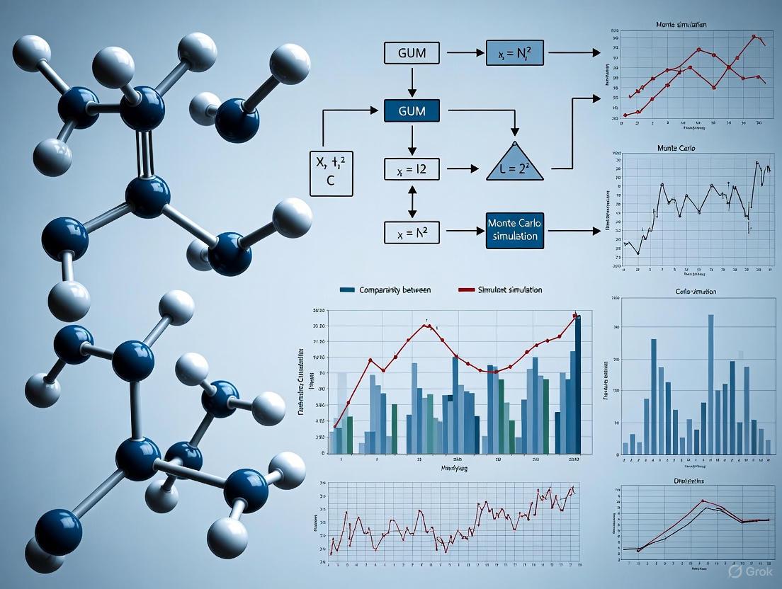
Visualization of Uncertainty Analysis Workflows

Generalized Uncertainty Analysis Framework

Uncertainty Analysis Decision Workflow

Experimental Protocol for Toxicity Testing

Toxicity Test Uncertainty Assessment

The Scientist's Toolkit: Essential Research Reagents and Materials

Table 3: Key Research Reagents and Materials for Uncertainty Analysis

Item	Function	Application Context
Activated Sludge	Biological medium for toxicity testing; contains microbial communities	Ecotoxicological testing (ISO 8192:2007) [4]
3,5-Dichlorophenol	Reference toxicant for method validation and calibration	Standardized toxicity testing [4]
Oxygen Probe	Measures dissolved oxygen concentration in biological systems	Respiration inhibition tests [4]
Temperature-Controlled Chambers	Maintain stable environmental conditions during testing	All biological measurements requiring temperature stability [4] [5]
Calibrated Flow Meters	Precisely measure and control airflow rates	Perspiration and respiration measurement systems [5]
Reference Materials	Provide traceability to stated references through unbroken chain of comparisons	Establishing measurement traceability [1]
Quality Control Materials	Monitor analytical performance and contribute to top-down uncertainty estimates	Routine medical laboratory testing [3]
DSM265	DSM265	DSM265 is a long-duration dihydroorotate dehydrogenase (DHODH) inhibitor for antimalarial research. For Research Use Only. Not for human use.
FN-1501	FN-1501, CAS:1429515-59-2, MF:C22H25N9O, MW:431.5 g/mol	Chemical Reagent

Critical Importance for Biomedical Data Integrity

In biomedical research and drug development, proper uncertainty quantification is not merely a technical requirement but a fundamental component of data integrity and reliability. The comparison of results from different laboratories, consistency assessment with reference values, and determination of suitability for clinical purpose all depend on robust uncertainty analysis [1].

Measurement uncertainty directly impacts risk assessment and decision-making processes throughout drug development. When measurement results lack proper uncertainty statements, decision risks increase significantly, potentially leading to incorrect conclusions about drug efficacy, safety profiles, or diagnostic accuracy [2]. This is particularly critical in biomedical contexts where decisions based on measurement data can affect patient diagnosis, treatment strategies, and regulatory approvals [6].

Furthermore, uncertainty analysis supports method validation and improvement by identifying dominant contributors to measurement variability. For instance, in toxicity testing, understanding that temperature tolerance, measurement interval, and oxygen probe accuracy account for over 90% of total uncertainty allows researchers to focus improvement efforts on these critical parameters [4]. This targeted approach to method optimization enhances both the quality and efficiency of biomedical research.

The choice between GUM and Monte Carlo methods should be guided by the specific characteristics of the measurement system, with GUM providing sufficient reliability for linear models with symmetric distributions, and Monte Carlo simulation offering superior performance for non-linear systems with asymmetric uncertainty distributions [4] [5]. As biomedical measurements continue to increase in complexity, the appropriate application of these uncertainty analysis methods will remain essential for maintaining data integrity across the research and development pipeline.

Foundational Principles of the GUM Framework

The Guide to the Expression of Uncertainty in Measurement (GUM) is an internationally recognized document published by the Joint Committee for Guides in Metrology (JCGM) that establishes standardized guidelines for evaluating and expressing uncertainty in measurement results [7]. This framework provides a systematic approach for quantifying uncertainties from various sources, including equipment limitations, environmental conditions, calibration procedures, and human factors, ensuring reliable and traceable measurement results [7].

The GUM operates on several core principles that form the backbone of its methodology. First, it introduces a clear categorization of uncertainty evaluation methods into Type A and Type B. Type A evaluation involves statistical analysis of measured data, typically through repeated observations, while Type B evaluation incorporates other knowledge such as manufacturer specifications, calibration certificates, or previous measurement data [8]. Second, the framework emphasizes the propagation of uncertainties through measurement models using the law of propagation of uncertainty (LPU), which is based on a first-order Taylor series approximation [5]. Third, it provides guidelines for expressing uncertainties using confidence intervals, expanded uncertainty, and coverage factors to indicate the level of confidence associated with measurement results [7].

A fundamental assumption underlying the GUM approach is that measurement models are linear or nearly linear and that the probability distributions involved can be adequately characterized by normal distributions or t-distributions [4] [5]. This assumption enables the use of simplified mathematical approaches for uncertainty propagation but also defines the boundaries beyond which the GUM method may become unreliable.

The GUM Workflow: A Step-by-Step Process

Implementing the GUM framework follows a systematic workflow that ensures comprehensive uncertainty analysis:

• Define the Measurand: Precisely specify the parameter to be measured and its units of measurement [7].
• Identify Uncertainty Sources: Document all components of the calibration process and accompanying sources of error, which may include calibration uncertainties, environmental conditions, electrical noise, and stability of the test setup [7].
• Quantify Uncertainty Components: Evaluate each source of error through Type A (statistical) or Type B (non-statistical) methods, determining probability distributions for each source [7] [8].
• Calculate Standard Uncertainties: Convert each uncertainty component to a standard uncertainty, expressed as a standard deviation [7].
• Determine Sensitivity Coefficients: Calculate how each input quantity affects the final measurement result [9].
• Construct Uncertainty Budget: Compile all components and their standard uncertainty calculations in a structured format [7].
• Combine Uncertainties: Apply the root-sum-of-squares (RSS) method to combine all standard uncertainty components [7].
• Calculate Expanded Uncertainty: Apply an appropriate coverage factor (typically k=2 for 95% confidence) to obtain the final expanded uncertainty [7].

This structured approach facilitates transparency and repeatability in uncertainty analysis, allowing metrologists to identify dominant uncertainty contributors and prioritize improvement efforts.

Experimental Comparison: GUM Versus Monte Carlo Methods

Performance Comparison in Practical Applications

Experimental studies across various fields have provided quantitative comparisons between GUM and Monte Carlo methods. The table below summarizes key findings from published research:

Table 1: Experimental Comparison of GUM and Monte Carlo Methods

Application Field	Measurement System	Key Findings	Reference
Toxicity Testing	ISO 8192:2007 oxygen consumption inhibition test	GUM results validated by MCS for oxygen consumption rates; Percentage inhibitions showed asymmetric distributions and were underestimated by GUM, especially at lower toxicant concentrations	[4]
Perspiration Measurement	Ventilated chamber sweat rate system	Measurement uncertainty: 6.81×10⁻⁶ kg/s (GUM) vs. 6.78×10⁻⁶ kg/s (MCS); Uncertainty percentage: 3.68% (GUM) vs. 3.66% (MCS)	[5]
Virtual CMM	Coordinate measurement machine simulation	For linear models with normally distributed errors: similar results; For non-linearity or biased data: propagation of distributions with bias correction provided most accurate results	[10]
Cadmium Measurement	Graphite furnace atomic absorption spectrometry	Main differences between methods attributed to calibration equation treatment	[5]
Electromagnetic Compatibility	EMC testing	No significant differences found between the two methods	[5]

Detailed Experimental Protocol: Toxicity Testing Case Study

The comparative analysis of GUM and Monte Carlo methods in toxicity testing followed a rigorous experimental protocol based on the ISO 8192:2007 method for determining oxygen consumption inhibition in activated sludge [4]:

Materials and Equipment:

• Activated Sludge: Sourced from a municipal wastewater treatment plant
• Reference Substance: 3,5-dichlorophenol (as recommended in ISO 8192:2007)
• Test Medium: Peptone (16 g), meat extract (11 g), urea (3 g), sodium chloride (0.7 g), calcium chloride dihydrate (0.4 g), magnesium sulphate heptahydrate (0.2 g), anhydrous potassium dihydrogen phosphate (2.8 g) dissolved in 1 L distilled/deionized water
• Additional Reagents: N-allylthiourea (ATU) solution (2.5 g/L) and 3,5-dichlorophenol (1 g/L)
• Equipment: Oxygen probe (FDO 925 WTW), multi-parameter meter (Multi 3430 WTW), magnetic stirrer (Rotilabo MH 15), aeration systems

Experimental Procedure:

• Activated sludge was settled at room temperature for one hour, decanted, and supernatant replaced with chlorine-free tap water (repeated four times for cleaning)
• Test mixtures were prepared with at least three test material concentrations (1.0 mg/L, 10 mg/L, 100 mg/L) and a blank control, plus four additional dilution levels for inhibition curves
• Mixtures were aerated (300-600 L/h) for 30 minutes before transfer to test vessels on magnetic stirrers
• Oxygen consumption was measured while maintaining temperature at 22±2°C and pH at 7.5±0.5
• Oxygen consumption rates were calculated using: ( Ri = \frac{\rho1 - \rho_2}{\Delta t} \times 60 ) mg/(L·h), where ρ₁ and ρ₂ represent oxygen concentrations at beginning and end of measurement range, and Δt is the time interval in minutes
• Evaluation included linear regression of oxygen consumption curves with prior outlier identification using Cook's Distance
• Inhibition curves were generated to determine EC50 values

Uncertainty Analysis Methodology: The study evaluated up to 29 uncertainty contributions using both GUM and Monte Carlo approaches. Dominant uncertainty contributors identified included temperature tolerance, measurement interval, and oxygen probe accuracy, accounting for over 90% of total uncertainty [4].

Research Reagent Solutions for Uncertainty Analysis

Table 2: Essential Research Materials for Uncertainty Analysis Experiments

Item	Function/Application	Example Specifications
Oxygen Probe	Measures oxygen consumption in toxicity tests	FDO 925 with Multi 3430 meter [4]
Temperature Control System	Maintains stable test environment	22±2°C maintenance capability [4]
Reference Substances	Provides calibrated comparison materials	3,5-dichlorophenol for toxicity testing [4]
Activated Sludge	Biological medium for toxicity assessment	Sourced from wastewater treatment plants [4]
Data Analysis Software	Implements GUM and MCS algorithms	Capable of statistical analysis and simulation [5]

Method Selection Guidelines and Limitations

The experimental evidence reveals clear guidelines for selecting between GUM and Monte Carlo methods based on measurement characteristics:

GUM Method is Preferred When:

• Measurement models are linear or nearly linear [10] [5]
• Error sources are normally distributed [10]
• Resources are limited, as GUM typically requires less computational time [5]
• The Welch-Satterthwaite formula can be adequately applied for effective degrees of freedom [5]

Monte Carlo Method is Superior When:

• Dealing with strong nonlinear models where Taylor series approximation becomes inaccurate [5]
• Probability distributions are asymmetric, as commonly occurs with percentage inhibition measurements [4]
• Models involve complex relationships that cannot be easily differentiated [9]
• Higher accuracy is required in uncertainty estimation, particularly with biased data analysis [10]

Key Limitations of Each Approach:

• GUM Limitations: Truncation errors from first-order Taylor series expansion in nonlinear models; potentially inaccurate assumption of normality; challenges in calculating effective degrees of freedom [5]
• Monte Carlo Limitations: Longer runtime requirements for complex cases; difficulty in selecting proper probability distribution functions; inability to visualize individual input contributions to overall uncertainty [5] [9]

The following diagram illustrates the decision process for selecting the appropriate uncertainty evaluation method:

The GUM framework provides a robust, standardized methodology for uncertainty evaluation that performs effectively across a broad spectrum of measurement applications. Its structured workflow, emphasizing systematic identification and quantification of uncertainty sources, enables metrologists to produce comparable, defensible measurement results across different laboratories and industries [7].

Experimental evidence confirms that GUM and Monte Carlo methods yield equivalent results for linear models with normally distributed errors [10] [5]. However, in cases involving significant nonlinearities, distribution asymmetries, or complex model structures, Monte Carlo simulation provides more accurate uncertainty estimation [4] [5]. The emerging research trend focuses on hybrid approaches that leverage the computational efficiency of GUM while incorporating Monte Carlo validation for critical applications requiring higher accuracy.

For researchers and drug development professionals, selecting the appropriate uncertainty analysis method requires careful consideration of model linearity, distribution characteristics, computational resources, and accuracy requirements. The experimental protocols and comparison data provided in this guide offer a foundation for making informed decisions that enhance the reliability of measurement results in pharmaceutical development and other scientific fields.

The Monte Carlo method, also known as Monte Carlo simulation or Monte Carlo experiments, is a broad class of computational algorithms that rely on repeated random sampling to obtain numerical results [11]. The fundamental concept involves using randomness to solve problems that might be deterministic in principle, making it particularly valuable for modeling phenomena with significant uncertainty in inputs [11] [12]. The method derives its name from the Monte Carlo Casino in Monaco, inspired by the gambling activities of the uncle of its primary developer, mathematician Stanisław Ulam [11] [13].

Monte Carlo methods have evolved from their origins during the Manhattan Project in the 1940s, where John von Neumann and Stanislaw Ulam systematically developed them to investigate neutron travel through radiation shielding [13] [12]. The method has since become an indispensable tool across diverse fields including physics, finance, engineering, and healthcare, enabling researchers to explore complex systems that are analytically intractable or too costly to experiment with directly [11] [14] [13].

Fundamental Principles of Monte Carlo Simulation

Core Concept and Theoretical Basis

At its essence, the Monte Carlo method is a numerical technique that predicts possible outcomes of uncertain events by employing probabilistic models that incorporate elements of uncertainty or randomness [12]. Unlike deterministic forecasting methods that provide definite answers, Monte Carlo simulation generates a range of possible outcomes each time it runs, offering a more realistic representation of real-world variability [12].

The method operates on the principle of ergodicity, which describes the statistical behavior of a moving point in an enclosed system that eventually passes through every possible location [12]. This becomes the mathematical foundation for Monte Carlo simulation, where computers run sufficient simulations to produce probable outcomes from different inputs [12]. The accuracy of results is proportional to the number of simulations performed, with higher iteration counts yielding more reliable predictions [12].

The Role of Probability Distributions

Probability distributions are fundamental components that represent the range of possible values for uncertain variables [12]. These statistical functions capture the inherent randomness in input parameters and are categorized as either discrete or continuous distributions:

• Normal distribution (bell curve): Symmetrically shaped like a bell, representing most real-life events where possibilities are highest at the median and decrease toward both extremes [12].
• Uniform distribution: Represents random variables with equal probability across the valid range, appearing as a horizontal flat line when plotted [12].
• Triangular distribution: Uses minimum, maximum, and most-likely values to represent random variables, with probability peaking at the most-likely value [12].
• Exponential distribution: Describes the time between events in a Poisson process or the distance a particle travels before interaction [13].

The Monte Carlo Simulation Process

Systematic Workflow

The Monte Carlo method typically follows a structured pattern comprising several distinct phases [11] [13] [12]:

Figure 1: Monte Carlo Simulation Workflow

Detailed Phase Explanation

• Define the Domain and Mathematical Model: Establish the system boundaries and develop equations describing relationships between input and output variables [12]. The mathematical model can range from basic business formulas to complex scientific equations and must accurately represent the system under investigation [12].

• Generate Random Inputs from Probability Distributions: Create large datasets of random samples (typically 100,000 or more) based on appropriate probability distributions [12]. This step utilizes pseudo-random number generators (RNGs), with modern algorithms like the Mersenne Twister providing high-quality random sequences while allowing reproducibility for testing and debugging [13].

• Perform Deterministic Computation: Execute the mathematical model using the generated random inputs [11]. Despite the random inputs, this computation is deterministic - the same inputs will always produce the same outputs [11] [12].

• Aggregate and Analyze Results: Collect all output data and perform statistical analysis to determine key parameters such as mean values, standard deviations, and confidence intervals [11] [12]. The results are typically presented as histograms or distribution graphs that show the continuous range of possible outcomes [12].

Comparative Analysis: Monte Carlo Simulation vs. GUM Framework

The Guide to the Expression of Uncertainty in Measurement (GUM) is an internationally recognized approach for estimating measurement uncertainties [4]. The GUM method relies on the law of uncertainty propagation and characterizes output quantities using normal or t-distributions [4]. For a response variable (y = y(x1, x2, \ldots, xn)), the combined uncertainty (uy) is calculated as:

[ uy = \sqrt{\sum{j=1}^{n}\left(\frac{\partial y}{\partial xj}u{xj}\right)^2 + 2\sum{j=1}^{n-1}\sum{i=j+1}^{n}\frac{\partial y}{\partial xi}\frac{\partial y}{\partial xj}u{xi,xj}} ]

where (u{xi,xj} = u{xi}u{xj}r{xi,xj}) and (-1 \leq r{xi,x_j} \leq 1) [15].

Key Differentiating Factors

Table 1: Fundamental Differences Between GUM and Monte Carlo Methods

Aspect	GUM Method	Monte Carlo Simulation
Theoretical Foundation	Law of uncertainty propagation & Taylor series expansion [4] [5]	Repeated random sampling & statistical analysis [11] [12]
Model Requirements	Differentiable models with known partial derivatives [5] [15]	Any computable model, including non-differentiable and black-box systems [11] [15]
Distribution Assumptions	Assumes normality or t-distributions for outputs [4] [5]	No distributional assumptions; empirically derives output distributions [12] [15]
Computational Approach	Analytical calculation using sensitivity coefficients [5] [16]	Numerical approximation through iterative sampling [11] [12]
Handling of Nonlinear Systems	Limited by first-order Taylor series approximation [5] [15]	Naturally accommodates strong nonlinearities without simplification [15]

Performance Comparison in Experimental Studies

Multiple experimental studies have directly compared the performance of GUM and Monte Carlo methods across various application domains:

Table 2: Experimental Comparison of GUM and Monte Carlo Methods

Application Domain	Key Findings	Reference
Toxicity Assessment (ISO 8192:2007)	GUM underestimated uncertainty at lower toxicant concentrations with asymmetric distributions; Monte Carlo provided accurate uncertainty quantification across all concentrations	[4]
Perspiration Measurement Systems	Both methods produced similar results (6.81 × 10⁻⁶ kg/s uncertainty), but Monte Carlo better captured system nonlinearities	[5]
Pressure Standard Effective Area	GUM required problematic simplifications for complex models; Monte Carlo enabled exact uncertainty calculations without approximations	[16]
Electronic Circuits (Sallen-Key Filter)	GUM produced inaccurate results for strongly nonlinear systems; Monte Carlo accurately quantified uncertainty despite nonlinearities	[15]
Biomedical Equipment	Monte Carlo provided more accurate results for nonlinear relationships, requiring increased trials for uncertainty stabilization	[5]

Output Analysis and Interpretation in Monte Carlo Simulations

Statistical Aggregation Techniques

The output analysis phase transforms raw simulation data into meaningful statistical insights through several key processes:

• Result Aggregation: Collecting all output values from multiple simulation runs for statistical processing [11]. For (n) simulations with results (ri), the empirical mean is calculated as (m = \frac{\sum{i=1}^{n} r_i}{n}) [11].

• Distribution Fitting: Analyzing the shape and characteristics of output distributions to identify patterns, asymmetries, and outliers [12]. This often involves creating histograms or probability density plots of the results [12].

• Confidence Interval Estimation: Determining ranges that contain the true value with specified probability [11]. The necessary sample size (n) for a desired accuracy (\epsilon) can be estimated using (n \geq s^2 z^2 / \epsilon^2), where (s^2) is the sample variance and (z) is the z-score corresponding to the desired confidence level [11].

Advanced Uncertainty Quantification

Figure 2: Uncertainty Quantification Process in Monte Carlo Analysis

Application in Drug Development and Healthcare

Pharmaceutical Research Implementation

Monte Carlo simulation has demonstrated particular value in drug development, where it addresses significant uncertainties in predictions of failure, cost overruns, and schedule variations [17]. The method enables dynamic modeling connecting preclinical stages through product launch, automatically reflecting time savings across dependent projects [17]. In healthcare more broadly, Monte Carlo methods have proven invaluable in treatment planning, risk assessment, and resource allocation [14].

Table 3: Research Reagent Solutions for Uncertainty Analysis

Research Tool	Function	Application Context
Random Number Generators	Generate pseudo-random sequences for sampling input distributions [13]	Foundation for all Monte Carlo simulations; critical for reproducibility
Probability Distribution Libraries	Provide mathematical models for various uncertainty patterns (normal, uniform, triangular, exponential) [12]	Represent different types of uncertain variables in experimental systems
Statistical Analysis Software	Perform aggregation and analysis of simulation outputs [12]	Calculate uncertainty metrics, confidence intervals, and sensitivity measures
Computational Parallelization Frameworks	Distribute simulation workload across multiple processors [11] [12]	Reduce computation time for large-scale uncertainty analyses
Sensitivity Analysis Tools	Identify dominant uncertainty contributors in complex systems [4]	Prioritize factors for measurement improvement and uncertainty reduction

Experimental Protocol for Pharmaceutical Uncertainty Analysis

A typical Monte Carlo implementation in drug development follows this structured protocol:

• Model Establishment: Define the complete drug development pathway as a mathematical model incorporating all stages from preclinical research to commercialization [17].

• Uncertainty Parameter Identification: Identify critical uncertain variables including success probabilities, development timelines, regulatory approval chances, and market dynamics [17].

• Probability Distribution Assignment: Assign appropriate probability distributions to each uncertain parameter based on historical data or expert judgment [17] [12].

• Simulation Execution: Run sufficient iterations (typically 10,000+) to obtain stable statistical results, utilizing parallel computing where necessary [17] [12].

• Portfolio Analysis: For multi-project portfolios, model dependencies between projects where success of one initiative signals others to proceed [17].

• Decision Support: Use resulting probability distributions of outcomes to support go/no-go decisions, resource allocation, and risk mitigation planning [17].

Comparative Advantages and Limitations

Benefits of Monte Carlo Simulation

• Complexity Handling: Capability to manage sophisticated models with dependencies within and across systems [17]
• Distribution Flexibility: No restrictive assumptions about input or output probability distributions [12] [15]
• Nonlinear System Compatibility: Accurate uncertainty quantification for strongly nonlinear systems where GUM fails [15]
• Comprehensive Uncertainty Capture: Ability to identify and model all viable outcomes from risks and opportunities [17]
• Visualization Capabilities: Generation of intuitive histograms and probability distributions for result communication [12]

Challenges and Computational Considerations

• Resource Intensity: Significant computational requirements, with simulations potentially taking hours or days to complete [11] [12]
• Input Sensitivity: Heavy dependence on appropriate input distributions and model structure [12]
• Implementation Complexity: Potential difficulty in selecting proper probability distribution functions for all input variables [5]
• Error Propagation: Inaccurate inputs necessarily lead to inaccurate outputs, as the method cannot compensate for fundamental model flaws [13]

The comparative analysis between GUM and Monte Carlo methods reveals distinct advantages for Monte Carlo simulation in complex, nonlinear systems prevalent in pharmaceutical research and drug development. While GUM provides an adequate analytical approach for simple, differentiable models with approximately normal output distributions, Monte Carlo simulation offers superior capability for handling real-world complexities, asymmetric distributions, and sophisticated dependency structures [4] [15].

For uncertainty analysis in drug development, where multiple interdependent factors contribute to overall project uncertainty and strategic decision-making, Monte Carlo methods provide a more robust and comprehensive framework [17]. The ability to model complete development pathways from preclinical research through commercialization, while dynamically capturing the impact of uncertainties across dependent projects, makes Monte Carlo simulation an indispensable tool for modern pharmaceutical researchers and development professionals [17].

In scientific research and drug development, quantifying the uncertainty associated with measurement results is not just good practice—it is a fundamental requirement for data integrity and regulatory compliance. The Guide to the Expression of Uncertainty in Measurement (GUM) outlines two primary methodological frameworks for this task: the analytical Law of Propagation of Uncertainty (LPU) and the numerical Statistical Sampling approach, most commonly implemented via Monte Carlo Simulation (MCS) [18] [19]. The LPU, rooted in differential calculus, provides an analytical solution, while MCS uses computational power to propagate distributions through random sampling [20]. This guide provides a detailed, objective comparison of these two approaches, supported by experimental data, to help researchers select the most appropriate method for their uncertainty analysis.

Theoretical Foundations and Methodologies

The core distinction between the two methods lies in their mathematical underpinnings and procedural execution.

Law of Propagation of Uncertainty (GUM Method)

The LPU is an analytical method based on the first-order Taylor series approximation of the measurement function [21] [18]. It is the internationally recognized approach detailed in the GUM [4].

• Mathematical Principle: For a measurand (Y = f(X1, X2, ..., XN)), the combined standard uncertainty (uc(y)) is calculated as shown in the equation below, where the partial derivatives (\partial f / \partial xi) are sensitivity coefficients, (u(xi)) are standard uncertainties of the inputs, and (u(xi, xj)) is the estimated covariance [21].
• Key Assumptions: The method assumes that the model can be satisfactorily linearized via its first-order Taylor expansion. It also generally characterizes the output quantity by a normal (Gaussian) distribution or a t-distribution [4]. The GUM procedure is based on the premise that all significant systematic errors have been identified and corrected [19].
• Complexity: The calculation of partial derivatives can become mathematically complex for highly non-linear models [20].

Statistical Sampling (Monte Carlo Simulation)

MCS is a numerical method that propagates uncertainties by simulating the measurement process a large number of times [19] [20].

• Mathematical Principle: MCS uses algorithmically generated pseudo-random numbers, forced to follow the probability density functions (PDFs) of the input quantities [19]. The model (Y = f(X1, X2, ..., X_N)) is evaluated repeatedly—often thousands or millions of times—with each evaluation using a new set of randomly sampled input values. The resulting distribution of output values directly provides the PDF of the measurand, from which its expectation, standard uncertainty, and coverage intervals can be derived empirically [19].
• Key Assumptions: MCS requires a reliable random number generator and a sufficient number of trials to ensure the output statistics converge to a stable value. It makes no linearity assumptions about the model [19].
• Implementation: For many medical laboratory applications, MCS can be implemented using readily available spreadsheets like Microsoft Excel, making it accessible without requiring advanced mathematical skills [19].

The fundamental workflows of these two methods are contrasted in the diagram below.

Comparative Analysis: Performance and Applications

The theoretical differences translate into distinct practical strengths, weaknesses, and ideal use cases for each method. The following table summarizes the key comparative characteristics.

Table 1: Key Differences Between LPU and Monte Carlo Simulation

Feature	Law of Propagation of Uncertainty (LPU)	Monte Carlo Simulation (MCS)
Core Approach	Analytical (based on differential calculus) [21]	Numerical (based on statistical sampling) [19] [20]
Mathematical Basis	First-order Taylor series approximation [22] [18]	Repeated random sampling from input Probability Density Functions (PDFs) [19]
Model Linearity	Assumes the model can be linearized; performance degrades with strong non-linearity [4]	Handles linear and non-linear models with equal validity [19] [4]
Output Distribution	Typically assumes a Normal or t-distribution for the output [4]	Empirically derives the output PDF, revealing asymmetry if present [19] [4]
Computational Demand	Low; single calculation	High; requires thousands to millions of model evaluations [20]
Handling Correlation	Explicitly included via covariance terms in the propagation formula [22] [21]	Can be handled by sampling from multivariate input distributions [20]
Ideal Use Cases	Relatively simple, linear or mildly non-linear models with well-behaved uncertainties [20]	Complex, highly non-linear models, or models producing asymmetric output distributions [4]

Experimental Data and Case Study Comparison

A 2025 study on toxicity assessment in wastewater treatment plants provides robust experimental data directly comparing both methods. The study quantified the measurement uncertainty of the ISO 8192:2007 method, which determines the inhibition of oxygen consumption in activated sludge, using both the GUM (LPU) and MCS approaches [4].

• Experimental Protocol: The investigation used activated sludge and 3,5-dichlorophenol as a reference substance. The core measurement was the oxygen consumption rate ((Ri)), calculated as ( Ri = \frac{\rho1 - \rho2}{\Delta t} \times 60 ) mg/L/h, where (\rho1) and (\rho2) are oxygen concentrations and (\Delta t) is the time interval [4]. The researchers evaluated up to 29 distinct uncertainty contributions, including temperature tolerance, measurement interval, and oxygen probe accuracy.
• Key Findings: The study concluded that for the calculated oxygen consumption rates, the results from the GUM method were successfully validated by MCS, confirming the LPU's reliability for this particular output [4]. However, for the final output of the analysis—the percentage inhibition—critical differences emerged. The MCS revealed that the percentage inhibitions at lower toxicant concentrations followed asymmetric distributions. The GUM method, which inherently assumes a symmetric output, underestimated the uncertainty in these cases [4].
• Interpretation: This case demonstrates that while the LPU is sufficient and computationally efficient for well-behaved, linear systems, MCS is indispensable for capturing the true uncertainty in complex, asymmetric systems often encountered in biological and pharmacological contexts.

Research Reagent Solutions for Uncertainty Analysis

The following table details key computational and statistical tools essential for implementing either uncertainty analysis approach.

Table 2: Essential Research Reagents & Tools for Uncertainty Analysis

Tool / Solution	Function in Uncertainty Analysis	Relevance to LPU or MCS
Mathematical Software (e.g., MATLAB, Mathematica)	Performs symbolic math for calculating partial derivatives required by the LPU, and provides libraries for random number generation for MCS [20].	Both
Statistical Packages (e.g., R, Python with SciPy/NumPy)	Provide built-in functions for statistical analysis, probability distribution fitting, and advanced sampling algorithms crucial for MCS [19].	Primarily MCS
Spreadsheet Software (e.g., Microsoft Excel)	Offers a accessible platform for implementing MCS using built-in random number functions and data analysis tools [19].	Primarily MCS
Probability Distribution Libraries	Provide predefined models (Normal, Rectangular, Triangular, etc.) to correctly characterize the knowledge about each input quantity [19].	Both
GUM Supplement 1 Documentation	The official guide for the propagation of distributions using a Monte Carlo method, serving as a key reference for MCS implementation [19] [4].	Primarily MCS

The choice between the Law of Propagation of Uncertainty and Statistical Sampling via Monte Carlo Simulation is not a matter of one being universally superior to the other. Instead, it is a strategic decision based on the complexity of the measurement model and the nature of the associated uncertainties.

The LPU is an efficient, established, and often sufficient analytical tool for linear or mildly non-linear models where the output can be reasonably assumed to follow a normal distribution. Its analytical nature makes it fast and well-suited for systems with a large number of inputs where MCS would be computationally expensive.

In contrast, MCS is a more powerful and robust numerical tool that should be employed for highly non-linear models, when input quantities have non-Gaussian distributions, or when the output distribution is suspected to be asymmetric [4]. It eliminates the need for complex linearization and provides a more empirically valid uncertainty estimate for complex systems, as evidenced by the toxicity testing case study.

For researchers and drug development professionals, this implies that the LPU remains a valuable tool for many routine analyses. However, for critical applications where model non-linearity is significant or the shape of the output distribution is unknown, MCS is the recommended and more reliable approach to ensure a complete and accurate assessment of measurement uncertainty.

Uncertainty analysis is a critical component in both laboratory accreditation and modern drug development, serving as a cornerstone for data reliability and regulatory decision-making. This guide examines the application of the Guide to the Expression of Uncertainty in Measurement (GUM) and Monte Carlo Simulation within frameworks like ISO/IEC 17025 and Model-Informed Drug Development (MIDD). By comparing these methodologies, we provide a structured analysis of their performance in quantifying measurement variability, which is essential for ensuring the validity of technical results and the safety and efficacy of pharmaceutical products.

The Guide to the Expression of Uncertainty in Measurement (GUM) is the internationally recognized benchmark for evaluating measurement uncertainty [4] [5]. It is based on the law of uncertainty propagation and uses a first-order Taylor series approximation to combine uncertainty contributions from all input quantities affecting a measurement. The GUM method assumes that the output quantity can be characterized by a normal or t-distribution, making it most reliable for linear or mildly nonlinear models [5].

In contrast, Monte Carlo Simulation (MCS) is a computational method recommended as a supplement to the GUM for more complex scenarios [4] [5]. It employs random sampling from the probability distributions of input quantities to build a numerical representation of the output quantity's distribution. This approach is particularly valuable for strongly nonlinear models or when the output distribution is expected to be asymmetric, as it does not rely on linear approximations [5].

The table below summarizes the core characteristics of each method.

Table: Foundational Principles of GUM and Monte Carlo Simulation

Feature	GUM Method	Monte Carlo Simulation
Core Principle	Analytical uncertainty propagation via first-order Taylor series [5].	Numerical approximation via random sampling from input distributions [4] [5].
Model Assumptions	Best for linear or mildly nonlinear models; assumes output is normal or t-distributed [5].	No linearity assumption; handles nonlinear models and asymmetric outputs effectively [4] [5].
Computational Demand	Generally low; calculated directly from a measurement equation.	Can be high, requiring a large number of trials (e.g., hundreds of thousands) for stable results [5].
Primary Application Context	Standardized measurement processes where models are well-understood and relatively linear.	Complex systems, nonlinear models, and cases where the shape of the output distribution is unknown or asymmetric [4].

Comparative Experimental Data and Performance

A 2025 study on toxicity assessment in wastewater treatment provides a direct, quantitative comparison of GUM and Monte Carlo Simulation for the ISO 8192:2007 method, which determines the inhibition of oxygen consumption in activated sludge [4].

Experimental Protocol for Uncertainty Analysis

The experimental setup and measurement procedure were established according to ISO 8192:2007. The key components of the protocol were [4]:

• Test Organism/Medium: Nitrified activated sludge from a municipal wastewater treatment plant was used, cleaned via settling and decanting.
• Reference Substance: 3,5-Dichlorophenol was used as the reference toxicant, prepared at a concentration of 1 g/L in distilled/deionized water.
• Test Mixture Preparation: A test mixture with multiple dilution levels (at least three concentrations plus a blank control) was prepared. The medium was aerated for 30 minutes before measurement.
• Measurement Conditions: The test environment was maintained at 22 ± 2 °C with a pH of 7.5 ± 0.5. Oxygen consumption was measured in a test vessel using a calibrated oxygen probe.
• Data Analysis: Oxygen consumption rates were calculated via linear regression of the oxygen concentration curves. Inhibition curves were then generated to determine the EC50 value.

The study evaluated up to 29 different uncertainty contributions [4]. The three dominant contributors were identified as:

• Temperature tolerance
• Measurement time interval
• Oxygen probe accuracy Together, these factors accounted for over 90% of the total measurement uncertainty [4].

Performance Comparison and Quantitative Outcomes

The study validated the GUM results for oxygen consumption rates using Monte Carlo Simulation, confirming the GUM's reliability for this specific output [4]. However, a critical divergence was observed for the calculation of percentage inhibition, particularly at lower toxicant concentrations.

Table: Comparative Performance in Toxicity Testing (ISO 8192:2007)

Analysis Output	GUM Method Results & Limitations	Monte Carlo Simulation Results & Advantages
Oxygen Consumption Rate	Results were validated by MCS, confirming reliability for this output [4].	Excellently aligned with GUM results, confirming its suitability for this specific metric [4].
Percentage Inhibition	Underestimated uncertainty, especially at lower toxicant concentrations. Struggled with asymmetric distributions [4].	Effectively captured the asymmetric distribution of results, providing a more realistic uncertainty estimate [4].
Key Finding	The GUM method's linearity assumption can lead to an underestimation of uncertainty in nonlinear, real-world biological systems [4].	Proven as a necessary alternative for systems exhibiting asymmetry, ensuring robust and realistic decision-making [4].

Regulatory Significance in ISO/IEC 17025 and Drug Development

Uncertainty Analysis in ISO/IEC 17025 Accreditation

For testing and calibration laboratories, ISO/IEC 17025:2017 mandates the assessment and reporting of measurement uncertainty (MU) as a critical requirement for demonstrating technical competence [23] [24]. Clause 7.6 of the standard specifically addresses the evaluation of measurement uncertainty [24].

A common mistake during assessments is the use of incomplete uncertainty models, for instance, including only calibration uncertainty while ignoring other key contributors like sample preparation, environmental conditions, and operator variability [24]. Such weaknesses have a domino effect, impacting the validity of decision rules, statements of conformity (Clause 7.8.6), and the ability to ensure the validity of results (Clause 7.7) [24]. The 2017 revision of the standard introduced a stronger emphasis on risk-based thinking, requiring laboratories to systematically address risks to the quality of their results [25] [26].

Uncertainty Analysis in Model-Informed Drug Development (MIDD)

In drug development, the principles of uncertainty analysis are embedded in Model-Informed Drug Development (MIDD). MIDD uses quantitative models to facilitate drug development and regulatory decision-making, aiming to reduce costly late-stage failures and accelerate patient access to new therapies [27].

A "Fit-for-Purpose" approach is central to MIDD, meaning the selected modeling and uncertainty analysis techniques must be well-aligned with the specific Question of Interest (QOI) and Context of Use (COU) at a given development stage [27]. For example:

• Physiologically Based Pharmacokinetic (PBPK) models require robust uncertainty and variability analysis to gain regulatory acceptance for predicting drug-drug interactions or extrapolating to special populations.
• Quantitative Systems Pharmacology (QSP) models are inherently complex, and uncertainty analysis is crucial for establishing confidence in their predictions for dose selection and trial design [27] [28].

The emerging use of Artificial Intelligence (AI) and Machine Learning (ML) in drug development further underscores the need for advanced uncertainty quantification. While AI projects can face high failure rates, generative AI shows high-value opportunities for accelerating modeling, simulation, and regulatory document creation, all of which rely on transparent uncertainty analysis [28].

Workflow and Implementation

The logical workflow for selecting and applying an uncertainty analysis method in a regulated laboratory or drug development setting is summarized below.

The Scientist's Toolkit: Essential Reagents and Materials

The following table details key materials and their functions based on the experimental protocol for the activated sludge respiration inhibition test (ISO 8192:2007), a representative method for uncertainty analysis in a biological system [4].

Table: Key Research Reagent Solutions for Uncertainty Analysis in Toxicity Testing

Item	Function in the Experimental Protocol
Activated Sludge	Serves as the biological matrix containing the microorganisms whose oxygen consumption is measured to assess toxicity [4].
3,5-Dichlorophenol	Used as a reference substance to standardize the toxicity test and validate the measurement method's performance [4].
Oxygen Probe	The primary sensor for measuring dissolved oxygen concentration in the test vessel over time; its accuracy is a major uncertainty contributor [4].
N-Allylthiourea (ATU)	A chemical inhibitor used to specifically suppress nitrification, allowing for the separate assessment of heterotrophic oxygen consumption inhibition [4].
Test Medium (Peptone, Meat Extract, Urea, Salts)	Provides essential nutrients and maintains ionic strength, creating a standardized environment for microbial activity during the test [4].
Temperature-Controlled Chamber	Maintains the test environment at a stable temperature (e.g., 22 ± 2 °C), as temperature fluctuation is a dominant uncertainty source [4].
Decanoyl-RVKR-CMK	Decanoyl-RVKR-CMK, MF:C34H66ClN11O5, MW:744.4 g/mol
GDC-0326	GDC-0326, CAS:1282514-88-8, MF:C19H22N6O3, MW:382.4 g/mol

Applied Uncertainty Analysis: Implementing GUM and Monte Carlo in Practice

Step-by-Step Guide to Conducting a GUM-Based Uncertainty Analysis

The Guide to the Expression of Uncertainty in Measurement (GUM) is an internationally recognized document that provides a standardized framework for evaluating and expressing measurement uncertainty. Developed by leading international standards organizations and first published in 1993, GUM establishes general rules applicable to a broad spectrum of measurements across different fields, from fundamental research to industrial applications [29] [7] [30]. The primary aim of GUM is to harmonize uncertainty evaluation practices, thereby ensuring reliability and facilitating the international comparison of measurement results [31] [29]. For researchers, scientists, and drug development professionals, applying a rigorous uncertainty analysis is not merely an academic exercise; it is a fundamental requirement for ensuring data integrity, assessing risk, and making defensible decisions based on measurement results. Compliance with standards such as ISO/IEC 17025, which requires uncertainty estimation for laboratory accreditation, further underscores its importance in regulated environments [4].

This guide is framed within a research context comparing the traditional GUM methodology, which relies on the law of propagation of uncertainty and a first-order Taylor series approximation, with the increasingly prevalent Monte Carlo Simulation (MCS) method, a computational technique that propagates distributions by performing random sampling [4] [5] [30]. While GUM is the established benchmark, its limitations in handling highly nonlinear models or asymmetric output distributions are key drivers for the adoption of MCS, as evidenced by recent comparative studies in environmental and biomedical fields [4] [5].

Fundamental Concepts of Measurement Uncertainty

Before embarking on a step-by-step analysis, it is crucial to understand the core concepts. Measurement uncertainty is defined as a "parameter, associated with the result of a measurement, that characterizes the dispersion of the values that could reasonably be attributed to the measurand" [4]. In simpler terms, it quantifies the doubt about the measurement's result.

The GUM framework classifies methods for evaluating uncertainty components into two types:

• Type A Evaluation: Method of evaluation by the statistical analysis of a series of observations. This typically involves calculating the mean and standard deviation from repeated measurements [32].
• Type B Evaluation: Method of evaluation by means other than statistical analysis of series of observations. This involves using scientific judgment, manufacturer's specifications, calibration certificates, or other prior knowledge to estimate an uncertainty component [32].

The final combined uncertainty, denoted as u_c(y), is a single standard deviation equivalent that encompasses all identified uncertainty sources. For reporting purposes, particularly to provide a confidence interval, an expanded uncertainty (U) is calculated by multiplying the combined uncertainty by a coverage factor (k). Common coverage factors are k=2 for approximately 95% confidence and k=3 for 99% confidence, under the assumption of a normal distribution [30].

The GUM Step-by-Step Uncertainty Analysis Procedure

The process of calculating measurement uncertainty via the GUM methodology can be systematically broken down into a series of sequential steps. Different sources consolidate these steps slightly differently, but the core workflow remains consistent [33] [29] [7]. The following seven-step procedure provides a robust framework for conducting an analysis.

Step 1: Specify the Measurand and Measurement Process

The first step involves creating a clear plan by specifying the measurement in detail.

• Action: Document a clear statement of what is being measured (the measurand), the mathematical formula or model used to calculate it, the specific method or procedure followed, and the equipment employed [33].
• Example: For a drug concentration in a powder mixture, the measurand is the weight fraction f, and the model is f = x / (x + y + z + ...), where x is the drug quantity and y, z,... are excipient quantities [34]. The equipment would include the balances used to weigh each component.

List every possible factor that could contribute to uncertainty in the final result.

• Common Sources: These include instrument resolution, repeatability, environmental conditions (e.g., temperature, humidity), operator bias, calibration uncertainties of equipment, and material stability [33] [7]. A cause-and-effect diagram (fishbone diagram) can be a useful tool in this step to visually map out all potential influencers.

Step 3: Quantify the Uncertainty Components

Assign a numerical value to each source identified in Step 2.

• For Type A uncertainties: Calculate the standard deviation of the mean from repeated measurements [32].
• For Type B uncertainties: Use available information. For example, if a balance has a readability of ±0.1 mg, the uncertainty is derived from this value. The GUM provides guidance on assigning probability distributions (e.g., normal for calibration certificates, rectangular for digital instrument resolution) to convert specifications into standard uncertainties [33] [30].

Step 4: Characterize Uncertainties and Determine Sensitivity Coefficients

• Characterize Distribution: Classify each component as Type A or Type B and state its probability distribution (e.g., Normal, Rectangular, Triangular) [33].
• Sensitivity Coefficients (c_i): These coefficients describe how much the output estimate (the measurand) changes with a small change in an input quantity. They are often determined from the partial derivative of the measurement model with respect to each input variable. For a model y = f(x1, x2, ...), the coefficient for x1 is c1 = ∂y/∂x1 [31] [34]. This step is crucial for converting input uncertainties into their contribution to the output's uncertainty.

Step 5: Convert Uncertainties to Standard Deviations

Ensure all uncertainty components are expressed as standard uncertainties, meaning they are in the form of a standard deviation. For a Type B evaluation with a rectangular distribution (due to a digital resolution of a), the standard uncertainty is u = a / √3 [33].

Step 6: Calculate the Combined Standard Uncertainty

Combine all the individual standard uncertainty components into a single combined standard uncertainty, u_c. This is typically done using the root-sum-square (RSS) method, which also incorporates the sensitivity coefficients [33] [7]. The general formula for non-correlated inputs is: u_c(y) = √[ (c1 ⋅ u(x1))² + (c2 ⋅ u(x2))² + ... ]

Step 7: Calculate the Expanded Uncertainty

To obtain an interval expected to encompass a large fraction of the distribution of values, calculate the expanded uncertainty, U. This is done by multiplying the combined standard uncertainty by a coverage factor, k [33] [30]. U = k â‹… u_c(y) The choice of k (typically 2 or 3) is based on the desired level of confidence (e.g., 95% or 99%) and the effective degrees of freedom of the measurement (often estimated via the Welch-Satterthwaite formula) [5].

The workflow for this entire 7-step process is summarized in the following diagram:

Experimental Protocols for Key Comparative Studies

To ground the GUM methodology in practical research, this section outlines the experimental protocols from key studies that have directly compared GUM and Monte Carlo methods.

Protocol 1: Toxicity Assessment in Wastewater Treatment

This study quantified the measurement uncertainty of the ISO 8192:2007 method, which determines the inhibition of oxygen consumption in activated sludge, a critical test for protecting biological processes in wastewater treatment plants [4].

• Experimental Setup: Activated sludge from a municipal plant was utilized. The test substance was 3,5-dichlorophenol, a reference toxicant. The test medium was prepared with peptone, meat extract, urea, and salts. A test mixture with multiple dilution levels was prepared and aerated before transfer to a test vessel.
• Measurement Procedure: Oxygen consumption was measured in the vessel using a calibrated oxygen probe placed on a magnetic stirrer. The environment was maintained at 22 ± 2 °C and a pH of 7.5 ± 0.5. The oxygen consumption rate (R_i) was calculated from the slope of the oxygen concentration decrease over time: R_i = (ρ1 - ρ2) / Δt * 60 mg/(L·h), where ρ1 and ρ2 are oxygen concentrations at the start and end of the linear range, and Δt is the time interval in minutes [4].
• Uncertainty Analysis: The study evaluated a total of 29 uncertainty contributions, including temperature tolerance, measurement time interval, and oxygen probe accuracy. Both GUM and MCS were applied to propagate these uncertainties for the oxygen consumption rate and the derived percentage inhibition.

Protocol 2: Perspiration Measurement System

This research evaluated the uncertainty of a system designed to measure human perspiration rate, a biomedical measurement system involving multiple input parameters [5].

• Experimental Setup: The system consisted of a ventilated chamber covering a skin area, with ambient air sucked in by a pump. The system was instrumented with a flow meter for airflow rate and sensors for temperature and relative humidity at the inlet and outlet.
• Measurement Procedure: The perspiration rate (G) was calculated indirectly from the measurements of airflow rate (m), inlet air density (ρ_in), and the absolute humidity of the inlet (d_in) and outlet (d_out) air, using the formula: G = m * (d_out - d_in) / ρ_in [5].
• Uncertainty Analysis: Uncertainty sources for each direct measurement (e.g., flow meter resolution and repeatability, sensor accuracy) were quantified. The propagation of these uncertainties through the perspiration rate equation was performed using both the GUM framework and Monte Carlo simulation, allowing for a direct comparison of the results and the underlying assumptions of each method.

Comparative Analysis: GUM vs. Monte Carlo Simulation

The following tables synthesize quantitative data and key characteristics from studies comparing GUM and Monte Carlo methods, highlighting the performance and applicability of each approach.

Table 1: Quantitative Results from Comparative Studies

Study Application	Key Inputs & Model	GUM Result	Monte Carlo Result	Key Finding
Toxicity Test (Oâ‚‚ Inhibition) [4]	29 inputs (Temp, Time, Probe). Nonlinear model for % inhibition.	Slightly underestimated uncertainty at low toxicant concentrations.	Revealed asymmetric distributions; provided more realistic uncertainty intervals.	GUM reliable for linear parts (Oâ‚‚ rate); MCS superior for nonlinear outputs (% inhibition).
Perspiration System [5]	Airflow, density, humidity. G = m*(d_out - d_in)/ρ_in.	Combined uncertainty: 6.81 × 10⁻⁶ kg/s.	Validated the GUM result for this specific model.	Both methods agreed well for this system, demonstrating GUM's adequacy for less complex models.
Drug Concentration in Mixture [34]	Masses of drug x and excipients y,z.... f=x/(x+y+z+...).	Relative uncertainty: df/f = (dx/x) * [1 + (n-1)f].	(Not applied in cited study)	Highlights GUM's use of a 1st-order Taylor series. Model shows uncertainty increases with number n of ingredients.

Table 2: Methodological Comparison of GUM and Monte Carlo Simulation

Feature	GUM Method	Monte Carlo Simulation
Theoretical Basis	Law of propagation of uncertainty; 1st-order Taylor series approximation [5].	Repeated random sampling from input probability distributions; numerical propagation [4] [30].
Model Complexity	Best suited for linear or mildly nonlinear models [5].	Handles highly nonlinear models and complex systems without simplification [4] [5].
Output Distribution	Assumes output is normal or t-distributed for expanded uncertainty [30].	Generates an empirical output distribution, revealing asymmetry if present [4] [30].
Computational Load	Low; analytical calculation.	High; requires thousands or millions of model evaluations to stabilize results [5].
Primary Limitation	Can produce errors for strong nonlinearities; may underestimate uncertainty for asymmetric distributions [5] [30].	Selection of correct input distributions is critical; runtime can be long for complex systems [5].

The relationship between the two methods and their optimal use cases is illustrated below. The GUM Supplement 1 officially endorses MCS as a complementary method, particularly for validating GUM results or when GUM's assumptions are violated [4] [5].

The Scientist's Toolkit: Essential Reagents and Materials

The following table details key reagents, materials, and software tools essential for conducting uncertainty analyses in experimental research, particularly in pharmaceutical and environmental contexts as cited.

Table 3: Essential Research Reagent Solutions and Software Tools

Item Name	Function / Role in Uncertainty Analysis	Example from Research Context
3,5-Dichlorophenol	Reference toxicant substance used to calibrate and validate bioassay responses.	Served as the reference substance in the ISO 8192:2007 toxicity test to ensure international comparability of inhibition results [4].
Activated Sludge	A complex microbial ecosystem used as the biological sensor in toxicity inhibition tests.	Sourced from a municipal wastewater plant; its oxygen consumption response to toxins is the core measurand [4].
N-allylthiourea (ATU)	Chemical inhibitor used to selectively suppress nitrification, allowing isolation of heterotrophic oxygen consumption.	Critical for modifying the standard test to measure specific inhibition pathways, adding a source of methodological uncertainty [4].
Calibrated Oxygen Probe	Sensor for measuring dissolved oxygen concentration, a direct source of measurement uncertainty.	A dominant uncertainty contributor; its accuracy, calibration, and resolution directly impact the oxygen consumption rate calculation [4].
SUNCAL Software	Free, open-source software for performing uncertainty calculations using both GUM and Monte Carlo methods.	Recommended for practical application, enabling researchers to perform the necessary statistical calculations and propagations [32].
Precision Balances	Instrument for determining the mass of drug and excipients; a primary source of uncertainty in formulation.	Its sensitivity (dx) is a key term in the uncertainty model for drug concentration in powder mixtures [34].
Glumetinib	Glumetinib, CAS:1642581-63-2, MF:C21H17N9O2S, MW:459.5 g/mol	Chemical Reagent
GNE-207	GNE-207, MF:C29H30N6O3, MW:510.6 g/mol	Chemical Reagent

This guide has detailed the step-by-step procedure for conducting a GUM-based uncertainty analysis, from specifying the measurand to reporting the expanded uncertainty. The comparative analysis with the Monte Carlo method reveals a clear landscape: the GUM framework provides a robust, analytically efficient, and standardized methodology that is perfectly adequate for a wide range of measurement problems, particularly those that are linear or only mildly nonlinear [5]. However, research demonstrates that for systems with significant nonlinearities or those that produce asymmetric output distributions, such as certain toxicity inhibition calculations, the GUM method can underestimate uncertainty [4]. In these cases, the Monte Carlo simulation offers a more powerful and reliable alternative, capable of revealing the true structure of the output uncertainty without relying on first-order approximations [5] [30].

For the modern researcher, the choice is not necessarily binary. The most rigorous approach, endorsed by the GUM Supplement 1, involves using the two methods in concert. One can use the GUM method for its efficiency and ease, while employing Monte Carlo simulation to validate the results, especially when operating near the boundaries of the GUM's applicability. This combined strategy ensures the highest level of confidence in uncertainty estimates, thereby strengthening the foundation of scientific conclusions and regulatory decisions in drug development and beyond.

Step-by-Step Guide to Implementing a Monte Carlo Simulation for Uncertainty

Uncertainty analysis is a cornerstone of reliable scientific research, ensuring that measurement results are accompanied by a quantifiable indicator of their reliability. For years, the Guide to the Expression of Uncertainty in Measurement (GUM) has provided the foundational framework for this analysis [19]. Its analytical, first-principles approach, however, presents challenges for complex, non-linear systems common in modern research. In response, the Monte Carlo Simulation (MCS) method has emerged as a powerful computational alternative [35]. This guide provides an objective comparison of these two methodologies, arming researchers and drug development professionals with the knowledge to select the appropriate tool for their uncertainty analysis needs. The core distinction lies in their approach: GUM uses an analytical method based on linear approximations and sensitivity coefficients, while MCS uses computational power to propagate distributions through random sampling, making it particularly suited for complex models [35] [4].

Theoretical Foundation: GUM and Monte Carlo Simulation

The GUM Framework

The GUM provides a standardized, internationally recognized procedure for uncertainty estimation [4] [19]. Its methodology is fundamentally analytical. It requires building a detailed mathematical model of the measurement process and calculating the combined standard uncertainty by determining the separate effect of each input quantity through sensitivity analysis, which often involves computing complex partial derivatives [35]. A fundamental premise of the GUM is the assumption that known systematic errors are identified and corrected early in the evaluation, with the remaining uncertainty comprising components from both random errors and the uncertainty of the corrections themselves [19]. For many linear models with well-understood inputs, this approach is robust and effective.

The Monte Carlo Simulation Method

In contrast, Monte Carlo Simulation is a probabilistic method that relies on repeated random sampling to estimate numerical results [36]. Instead of solving a deterministic problem analytically, MCS uses randomness to simulate a process thousands of times, thereby building a distribution of possible outcomes [35]. This process involves defining probability distributions for all input variables and then running a large number of iterations, where for each iteration, values for the inputs are randomly drawn from their respective distributions and used to compute an output value [37] [38]. The resulting collection of output values forms a probability distribution, from which uncertainty estimates can be directly derived without the need for complex differential equations [19].

Comparative strengths and limitations

The table below summarizes the core characteristics of each method.

Table 1: Fundamental Comparison of GUM and Monte Carlo Methods

Feature	GUM Method	Monte Carlo Simulation
Core Approach	Analytical (first-principles)	Computational (numerical sampling)
Mathematical Basis	Law of uncertainty propagation; Taylor series expansion	Repeated random sampling & statistical analysis
Handling Non-Linearity	Can be unreliable; neglects higher-order terms [35]	Naturally accounts for all non-linearities [35]
Handling Correlated Inputs	Complex and sometimes unreliable [35]	Can directly model correlation effects [35]
Output Distribution	Assumes/outputs a standard (e.g., normal, t-) distribution [4]	Empirically generates any output distribution, reveals asymmetries [4]
Skill Requirement	Advanced mathematical skills for derivatives [19]	Less advanced math; requires programming/software knowledge [19]

Experimental Comparison: A Case Study in Toxicity Testing

Experimental Protocol and Methodology

A 2025 study quantifying the measurement uncertainty of the ISO 8192:2007 method, which determines the inhibition of oxygen consumption in activated sludge, provides robust experimental data for a direct comparison [4]. The study evaluated up to 29 separate uncertainty contributions.

• Measured System: Inhibition of oxygen consumption in activated sludge using 3,5-dichlorophenol as a reference substance [4].
• Key Measured Parameters: Oxygen consumption rate and percentage inhibition [4].
• Methodology: The uncertainty of the method was evaluated using both the GUM guideline and Monte Carlo Simulation (validated with 100,000 iterations) to facilitate a direct comparison of the results [4].
• Dominant Uncertainty Sources: The study identified temperature tolerance, measurement interval, and oxygen probe accuracy as the dominant contributors, accounting for over 90% of the total uncertainty [4].

Quantitative Results and Data Comparison

The experimental data allows for a clear, objective comparison of the outputs from both methods.

Table 2: Experimental Results from Toxicity Testing Uncertainty Analysis

Analysis Aspect	GUM Result	Monte Carlo Simulation Result	Comparative Insight
Oxygen Consumption Rate	Calculated combined standard uncertainty	Validated GUM results [4]	Both methods show strong agreement for this linear(ish) output [4].
Percentage Inhibition	Underestimated uncertainty, especially at low concentrations [4]	Revealed asymmetric distributions; provided realistic uncertainty [4]	GUM failed to capture the true risk for non-linear, asymmetric systems [4].
Impact of Correlations	Considered; had minimal impact on outcomes [4]	Considered; had minimal impact on outcomes [4]	For this specific experiment, correlation was not a decisive factor.
Overall Conclusion	Reliable for linear models and symmetric uncertainties.	Necessary for asymmetric outputs and non-linear models [4].	MCS revealed GUM's limitations in complex scenarios.

A Step-by-Step Protocol for Implementing a Monte Carlo Simulation

The following workflow diagram outlines the general process for conducting a Monte Carlo Simulation, which can be adapted to various scientific applications.

Step 1: Identify the Transfer Equation

The first step is to define the quantitative model that represents the process or relationship you wish to explore. This mathematical expression is known as the "transfer equation" [38].

• For Engineering/Physics: This may be a known formula. For example, in a pump design, flow can be calculated as: Flow = π(D/2)² * L * RPM, where D is piston diameter, L is stroke length, and RPM is strokes per minute [38].
• For Complex/Novel Processes: If no established formula exists, a model can be created from a Designed Experiment (DOE) or regression analysis. For instance, a response surface DOE for an electrocleaning process yielded the transfer equation: Roughness = 957.8 − 189.4(Vdc) − 4.81(ASF) + 12.26(Vdc²) + 0.0309(ASF²) [38].

Step 2: Define the Input Parameters

For each factor in your transfer equation, you must define its probability distribution. The accuracy of the simulation is highly dependent on the quality of this input data [37].

• Select Probability Distributions: Common distributions include:
  • Normal Distribution: Characterized by mean (μ) and standard deviation (σ). Used for many natural phenomena and measurements subject to small random errors [19].
  • Rectangular (Uniform) Distribution: Defined by a lower and upper limit (±a). Used when the probability of any value within the range is equal. Its standard deviation is a/√3 [19].
  • Triangular Distribution: Also defined by limits (±a), but with a peak at the central value. Its standard deviation is a/√6 [19].
• Example from Manufacturing: In the piston pump example, inputs were defined as normally distributed: Piston diameter (mean=0.8 cm, SD=0.003 cm), Stroke length (mean=2.5 cm, SD=0.15 cm), RPM (mean=9.549, SD=0.17) [38].

Step 3: Set Up and Run the Simulation

This step involves running a large number of iterations to simulate the long-term behavior of the process.

• Number of Iterations: For reliable results, a large number of iterations is required—typically on the order of 100,000 [38]. This large sample size ensures the output distribution is stable and representative.
• Execution: Software tools automatically generate the specified number of random data sets for the input parameters based on their defined distributions. Each of these 100,000 simulated scenarios is then calculated using the transfer equation to produce 100,000 potential outcomes [38].

Step 4: Analyze the Process Output

The final step is to interpret the generated output data to make informed decisions.

• Visualize the Distribution: Plot the results in a histogram to visualize the full range of possible outcomes and their probabilities [36] [37].
• Calculate Key Statistics: Determine the mean, standard deviation, and percentiles (e.g., the 5th and 95th percentile to define a 90% confidence interval) of the output distribution [38].
• Draw Insights: Assess the likelihood of different scenarios, identify risks, and plan contingencies. For example, the pump simulation revealed a flow standard deviation of 0.756 ml, far exceeding the target of 0.2 ml, indicating a need for design refinement before production [38].

The Scientist's Toolkit: Essential Reagents and Materials

For researchers implementing these methods, particularly in biochemical contexts like the cited study, the following tools and reagents are essential.

Table 3: Key Research Reagent Solutions for Uncertainty Analysis

Reagent / Material	Function / Application	Example from Literature
Activated Sludge	The biological medium for assessing toxicity on microbial processes.	Sourced from a municipal wastewater treatment plant [4].
3,5-Dichlorophenol	A reference substance used to validate and calibrate toxicity tests.	Recommended as a reference substance in ISO 8192:2007 [4].
Oxygen Probe	Critical for measuring dissolved oxygen concentration over time.	FDO 925 model from WTW, used with a Multi 3430 meter [4].
N-allylthiourea (ATU)	An inhibitor used to selectively suppress nitrification, allowing for specific oxygen consumption measurements.	Dissolved at 2.5 g/L in distilled/deionized water [4].
Test Medium (Peptone, etc.)	Provides a standardized nutrient source to maintain microbial activity during testing.	Contains peptone, meat extract, urea, and salts [4].
Statistical Software	Enables the execution of thousands of MCS iterations and data analysis.	Tools like Minitab Engage/Workspace, or spreadsheet software like Excel [19] [38].
GNF7686	GNF7686, CAS:442567-43-3, MF:C15H13N3O, MW:251.289	Chemical Reagent
GNF-8625	GNF-8625, CAS:1196546-33-4, MF:C31H30FN7O, MW:535.63	Chemical Reagent

The choice between GUM and Monte Carlo Simulation is not a matter of which is universally better, but which is more appropriate for a specific application. The GUM method is a powerful, established tool for linear models and systems where uncertainties are well-behaved and symmetric. Its analytical nature is efficient and does not require significant computational resources. However, for complex systems characterized by non-linearities, correlated inputs, or those that produce asymmetric output distributions, the Monte Carlo Simulation method is demonstrably superior [35] [4]. It provides a more realistic and reliable uncertainty estimate under these conditions, albeit at the cost of greater computational effort. For researchers in drug development and other advanced scientific fields where models are often complex, MCS offers a robust and accessible means to achieve a higher standard of measurement reliability.

The accurate quantification of trace levels of cadmium in water is a critical task in environmental monitoring and public health protection. Graphite Furnace Atomic Absorption Spectrometry (GFAAS) is a widely employed technique for this purpose due to its high sensitivity and low detection limits [39]. However, the reliability of any analytical measurement must be assessed through a rigorous evaluation of its uncertainty, which quantifies the doubt surrounding the result [4] [40]. This case study examines the direct determination of cadmium in water by GFAAS, with a specific focus on comparing two established approaches for uncertainty evaluation: the Guide to the Expression of Uncertainty in Measurement (GUM) framework and the Monte Carlo Simulation (MCS) method [41]. The research is situated within a broader thesis investigating the comparative performance of these two methodologies in analytical chemistry, highlighting their applications, limitations, and practical implications for measurement science.

Methodologies for Uncertainty Evaluation

The GUM Uncertainty Framework

The GUM provides a standardized, internationally recognized methodology for evaluating and expressing measurement uncertainty [4] [40]. Its application involves a systematic process of identifying and quantifying all significant sources of uncertainty, which are then combined using the law of propagation of uncertainty. For GFAAS analysis, key uncertainty sources include preparation of calibration standards, instrument precision (repeatability), and the calibration curve generated by least squares regression [41]. The GUM framework typically characterizes the output quantity (the measurand) by a Gaussian or a t-distribution to determine an expanded uncertainty at a specified confidence level, usually 95% [41].

The Monte Carlo Simulation Method

The Monte Carlo Method offers a computational alternative for propagating uncertainty, as detailed in a Supplement to the GUM [41]. This approach involves assigning probability distributions to all input quantities and then randomly sampling from these distributions a large number of times (e.g., hundreds of thousands or millions) through a mathematical model of the measurement process [4] [40]. The result is a discrete representation of the probability distribution for the output quantity, from which the uncertainty can be directly derived. This method is particularly advantageous for complex, non-linear models or when the output distribution is not symmetric [4] [40].

Experimental Protocol for Cadmium Measurement by GFAAS

Instrumentation and Analytical Procedure

The experimental data for this case study is derived from the direct determination of cadmium in water using GFAAS [41]. The core of the GFAAS system is a graphite tube, which is heated in controlled stages (drying, pyrolysis, atomization, clean-out) to produce a transient cloud of free cadmium atoms [42]. A hollow cathode lamp emits light at cadmium's specific resonance wavelength (e.g., 228.8 nm), and a detector measures the absorption of this light, which is proportional to the cadmium concentration according to the Beer-Lambert law [42]. To manage the complex seawater matrix, techniques such as matrix modification (e.g., with palladium and magnesium nitrates) and background correction (e.g., Zeeman effect) are often essential to mitigate interferences and stabilize the analyte during pyrolysis [39] [42]. The temperature program must be carefully optimized to separate the cadmium signal from the background matrix effectively [39].

Key Reagents and Materials

Table 1: Essential Research Reagents and Materials for GFAAS Analysis of Cadmium

Item	Function	Example/Specification
Graphite Tubes	Sample holder and atomizer; must be resistant to high temperatures and chemical corrosion [42].	Pyrolytically coated graphite tubes [42].
Matrix Modifiers	Chemical agents that stabilize the analyte and modify the sample matrix to reduce interferences during the pyrolysis stage [39] [42].	Palladium nitrate, Magnesium nitrate [39].
Cadmium Standard Solutions	Used for instrument calibration to establish the relationship between absorbance and concentration [43].	Certified reference materials in appropriate acid matrix [43].
High-Purity Gases	Create an inert atmosphere within the graphite furnace to prevent tube oxidation and sample decomposition [42].	Argon (99.99% purity) [42].
Hollow Cathode Lamps	Source of monochromatic light at the specific resonance wavelength of cadmium [42].	Element-specific cadmium lamp [42].
Ultrapure Acids & Reagents	For sample preparation and dilution; purity is critical to minimize blank contamination [44].	Nitric acid, trace metal grade [44].

Results and Comparative Uncertainty Analysis

Quantitative Comparison of GUM and MCS

The application of both the GUM framework and the Monte Carlo Method to the determination of cadmium at a concentration level of 3.01 μg/L yielded the following results for expanded uncertainty at a 95% confidence level [41]:

Table 2: Comparison of Expanded Uncertainty Results for Cadmium Measurement (at 3.01 μg/L)

Uncertainty Evaluation Method	Expanded Uncertainty (μg/L)	Key Characteristics
GUM Uncertainty Framework	±0.20 μg/L	Slightly overestimates uncertainty (by ~10%) in this case; relies on approximations for calibration curve uncertainty [41].
Monte Carlo Method (MCS)	±0.18 μg/L	Provides a more realistic estimate; directly models the measurement process without some GUM assumptions [41].

The study found that the GUM framework overestimated the uncertainty by approximately 10% compared to the MCS result [41]. This discrepancy was primarily attributed to the approximation used by the GUM method for estimating the standard uncertainty associated with the calibration curve produced by least-squares regression [41]. Even when additional uncertainty sources, considered negligible by the GUM approach, were included in the MCS model, the result remained stable at ±0.18 μg/L, demonstrating the robustness of the simulation [41].

Workflow for Uncertainty Analysis in GFAAS

The following diagram illustrates the logical workflow and key differences between the GUM and Monte Carlo approaches for uncertainty analysis in this context.

This case study demonstrates that both the GUM framework and the Monte Carlo Method are viable for evaluating the measurement uncertainty of cadmium in water using GFAAS. For this specific analytical application, the GUM framework proved to be adequate, albeit resulting in a slight overestimation of the uncertainty [41]. The Monte Carlo Method, while potentially more computationally intensive, offers a more direct and flexible approach that avoids some of the assumptions and limitations inherent in the GUM framework [41]. The findings affirm that the choice of uncertainty evaluation method can impact the reported uncertainty, a critical consideration for regulatory compliance and method validation in environmental and pharmaceutical analysis [43] [4] [40]. This reinforces the thesis that MCS is a powerful tool for validating GUM results, particularly in cases involving complex models or asymmetric distributions.

In biomedical engineering, the reliability of measurement data is paramount, as it directly influences diagnostic decisions, treatment strategies, and product development. Measurement uncertainty is a key parameter for expressing measurement results and reliability, allowing researchers to quantify factors affecting outcomes and compare results across different laboratories [5]. The Guide to the Expression of Uncertainty in Measurement (GUM) established fundamental concepts and principles for developing uncertainty models and has become an internationally recognized approach [4] [45]. However, GUM has recognized limitations, particularly for complex, non-linear systems, leading to the development of alternative methods such as Monte Carlo Simulation (MCS) [5].

Perspiration measurement systems represent a critical biomedical application where uncertainty analysis is essential. These systems monitor sweat rate and composition to provide non-invasive insights into physiological states, hydration levels, and metabolic health [46] [47]. With the wearable sweat sensor market projected to grow from USD 59.2 million in 2024 to USD 1.1 billion by 2034, rigorous uncertainty analysis ensures these devices deliver reliable data for clinical and consumer applications [46]. This case study examines the application of both GUM and Monte Carlo methods for evaluating measurement uncertainty in a perspiration measurement system, providing a comparative analysis of their methodologies, results, and practical implications for researchers and drug development professionals.

Theoretical Framework: GUM and Monte Carlo Methods

The GUM Methodology

The GUM framework provides a systematic approach to uncertainty quantification based on mathematical modeling of all significant uncertainty sources. This methodology involves identifying and categorizing uncertainty contributions, then propagating them through a measurement model using the law of uncertainty propagation and a first-order Taylor series approximation [45]. The result is a combined standard uncertainty that can be expanded to provide an interval containing the true value with a specified probability [4]. GUM is particularly effective for linear models or those with slight nonlinearities, and it forms the foundation for uncertainty evaluation in accredited calibration and testing laboratories [45].

Monte Carlo Simulation Methods

The Monte Carlo method, formalized in the GUM Supplement 1, provides a computational alternative to the analytical GUM approach. MCS uses random sampling from probability distributions of input quantities to numerically simulate the measurement model thousands of times [5] [4]. This generates a probability distribution for the output quantity, from which uncertainty intervals can be directly derived. MCS is particularly valuable for complex models with significant nonlinearities, correlated inputs, or asymmetric output distributions where the GUM's linear approximations may prove inadequate [4] [48].

Fundamental Uncertainty Categories

In computational modeling, uncertainties are typically categorized as either aleatory or epistemic. Aleatory uncertainty refers to the inherent variation in a system caused by random effects that cannot be reduced, such as biological variability between subjects. Epistemic uncertainty stems from lack of knowledge about the system behavior and can theoretically be reduced through improved models or additional data [49] [48]. Both GUM and Monte Carlo methods can address these uncertainty types, though their approaches and effectiveness differ depending on the measurement context.

Table 1: Comparison of GUM and Monte Carlo Methodologies

Characteristic	GUM Method	Monte Carlo Simulation
Theoretical Basis	Law of uncertainty propagation with first-order Taylor series	Random sampling from probability distributions
Model Requirements	Explicit measurement function with continuous first derivatives	Computational model implementation
Computational Approach	Analytical calculation	Numerical simulation
Output Distribution	Assumes normality or t-distribution	Empirically derived from simulations
Handling of Nonlinearities	Limited by first-order approximation	Naturally accommodates full nonlinearities
Treatment of Correlations	Requires explicit correlation coefficients	Can implicitly handle correlations through joint distributions

Experimental Setup: Perspiration Measurement System

System Description and Measurement Principle

The perspiration measurement system under investigation employs a ventilated chamber design where ambient air is drawn into the chamber by an air pump, with the inlet air disturbed to ensure uniform mixture with humidity evaporated from human skin [5]. The system measures multiple parameters: airflow rate via a flow meter, and temperature and relative humidity of both inlet and outlet air using specialized sensors. The fundamental measurement principle relies on calculating absolute humidity from temperature and relative humidity measurements, then determining the perspiration rate (ṁ_sw) through mass balance equations considering airflow rate, air density, and the difference between outlet and inlet absolute humidity [5].

The perspiration rate is calculated using the equation: ṁsw = ṁa * (ρa.out * Yout - ρa.in * Yin) Where ṁa represents the airflow rate, ρa is air density, and Y is absolute humidity, with subscripts indicating inlet (in) and outlet (out) conditions [5].

The comprehensive uncertainty analysis identified multiple contributors to measurement uncertainty, which were systematically categorized and quantified:

Table 2: Uncertainty Components in the Perspiration Measurement System

Uncertainty Source	Measurement Component	Distribution Type	Evaluation Method
Sensor Resolution	Airflow meter display	Uniform	Type B
Measurement Repeatability	All sensors	Normal	Type A
Calibration Accuracy	Temperature and RH sensors	Normal	Type B
Environmental Factors	Temperature tolerance	Rectangular	Type B
Temporal Variations	Measurement interval	Rectangular	Type B
Physical Properties	Air density calculation	Normal	Type B

Research Reagent Solutions and Essential Materials

Table 3: Key Research Materials and Their Functions in Perspiration Measurement

Material/Component	Function	Specification/Notes
Temperature Sensors	Measure inlet/outlet air temperature	Calibrated to specified tolerance
Relative Humidity Sensors	Measure inlet/outlet air humidity	Calibrated to specified tolerance
Airflow Meter	Measure volumetric flow rate	4-decimal place resolution
Air Pump	Draw air through ventilation chamber	Provides consistent airflow
Ventilation Chamber	Interface with human skin	Ensures uniform air mixture
Data Acquisition System	Record sensor measurements	Specific sampling interval
Reference Materials	Calibration and validation	Traceable to national standards

Application of GUM and Monte Carlo Methods

GUM Implementation for Uncertainty Analysis

The GUM method was applied to the perspiration measurement system by first developing a detailed measurement model that expressed the perspiration rate as a function of all input quantities. Each uncertainty component was quantified either through Type A evaluation (statistical analysis of repeated measurements) or Type B evaluation (based on manufacturer specifications, calibration certificates, or scientific principles) [5] [45]. The combined standard uncertainty was calculated by propagating these individual uncertainties through the measurement model using the law of propagation of uncertainties, which involves partial derivatives and accounts for correlations between input quantities where necessary [4]. Finally, an expanded uncertainty was determined by multiplying the combined standard uncertainty by a coverage factor corresponding to the desired level of confidence, typically 95% (k=2) [5].

For the perspiration measurement system, the GUM analysis quantified the uncertainty contribution from each source. The airflow rate uncertainty was assessed considering both resolution (uniform distribution) and repeatability (normal distribution from 30 readings) [5]. Air density uncertainty was derived from the ideal gas law, considering uncertainties in temperature, pressure, and relative humidity measurements. The absolute humidity uncertainty was calculated from temperature and relative humidity measurements, accounting for sensor calibration accuracy and resolution [5].

Monte Carlo Simulation Implementation

The Monte Carlo approach involved defining probability distribution functions for each input quantity based on their uncertainty characteristics [5] [4]. For the perspiration measurement system, normal distributions were typically used for calibration uncertainties, uniform distributions for resolution limitations, and rectangular distributions for environmental tolerance effects. The measurement model was then evaluated repeatedly (typically 10^5 to 10^6 iterations) with random samples drawn from these input distributions [4]. This process generated a probability distribution for the output quantity (perspiration rate), from which the uncertainty interval was directly determined by calculating appropriate percentiles (e.g., 2.5th and 97.5th percentiles for a 95% coverage interval) [5] [4].

The MCS implementation specifically addressed the nonlinearities in the perspiration measurement model that the GUM approach approximated through first-order linearization. This included the nonlinear relationship between temperature and saturated vapor pressure in humidity calculations, and the multiplicative nature of the mass balance equation [5]. The simulation also naturally handled the propagation of distributions without requiring explicit correlation coefficients between input quantities, as any correlations were implicitly maintained through the sampling process [4].

Comparative Workflow Visualization

The following diagram illustrates the comparative workflows for implementing GUM and Monte Carlo methods in uncertainty analysis of the perspiration measurement system:

GUM and Monte Carlo Method Workflows

Results and Comparative Analysis

Quantitative Uncertainty Results

The application of both GUM and Monte Carlo methods to the perspiration measurement system yielded the following comparative results:

Table 4: Comparative Results of GUM and Monte Carlo Methods

Performance Metric	GUM Method	Monte Carlo Method
Total Measurement Uncertainty	6.81 × 10^(-6) kg/s	6.79 × 10^(-6) kg/s
Uncertainty Percentage	6.12%	6.10%
Computational Time	Seconds	Minutes to Hours
Handling of Nonlinear Effects	Approximated	Exact
Distribution Shape	Assumed symmetric	Empirically derived
Key Uncertainty Contributors	Temperature tolerance, measurement interval, oxygen probe accuracy	Temperature tolerance, measurement interval, oxygen probe accuracy

Methodological Strengths and Limitations

Both methods identified temperature tolerance, measurement interval, and sensor accuracy as dominant uncertainty contributors, collectively accounting for over 90% of the total uncertainty in the perspiration measurement system [5] [4]. This consistency in identifying major uncertainty sources validates both approaches for sensitivity analysis and provides clear guidance for measurement system improvement.

The GUM method demonstrated computational efficiency, providing results in seconds compared to the potentially lengthy runtime of Monte Carlo simulations for complex models [5]. However, this efficiency came at the cost of approximation accuracy, particularly for the nonlinear aspects of the perspiration measurement model. The GUM approach also relied on the assumption of normality for calculating expanded uncertainty, which may not be appropriate for all measurement scenarios [5] [4].

The Monte Carlo method provided more accurate uncertainty quantification for nonlinear models without requiring simplifying assumptions about the output distribution [5] [4]. This capability proved particularly valuable for percentage inhibition calculations at lower toxicant concentrations in related biomedical applications, where asymmetric distributions were observed and GUM methods tended to underestimate uncertainty [4]. The main limitations of MCS included longer computational times for complex models and the challenge of selecting appropriate probability distribution functions for all input quantities [5].

Implications for Biomedical Applications

Practical Guidance for Method Selection

Based on the comparative analysis, method selection depends on specific application requirements. The GUM method is recommended for relatively linear systems, routine measurements requiring rapid results, and initial uncertainty assessments where computational simplicity is prioritized [5] [45]. Monte Carlo simulation is preferable for complex, highly nonlinear systems, critical applications where distributional assumptions must be verified, and cases where asymmetric uncertainty intervals are expected [5] [4].

For perspiration measurement systems specifically, the choice depends on the required uncertainty precision and available computational resources. While both methods produced similar results for the main perspiration rate calculation, Monte Carlo provided more accurate uncertainty intervals for derived quantities like percentage inhibition, which exhibited asymmetric distributions [4]. This distinction is particularly relevant for biomedical applications where measurements near detection limits or threshold values are common.

Relevance to Wearable Sweat Sensor Development

The uncertainty analysis methodologies applied to the laboratory perspiration measurement system directly inform the development and validation of commercial wearable sweat sensors. The wearable sweat sensor market is experiencing rapid growth, projected to expand from USD 59.2 million in 2024 to USD 1.1 billion by 2034, driven by demand from athletes, fitness enthusiasts, and healthcare applications [46] [50]. These devices monitor biomarkers including electrolytes, glucose, cortisol, and ethanol to provide insights into hydration, metabolic status, and stress levels [50] [47].

Rigorous uncertainty quantification is essential for addressing key market challenges, including accuracy concerns and limited clinical validation [46]. Understanding and minimizing measurement uncertainty through methods like GUM and Monte Carlo simulation supports clinical adoption by providing transparent reliability assessments [5] [45]. Furthermore, uncertainty analysis guides sensor optimization by identifying dominant uncertainty contributors, thus directing research and development efforts toward parameters with the greatest impact on measurement quality [5] [4].

This case study demonstrates that both GUM and Monte Carlo methods provide effective frameworks for quantifying uncertainty in perspiration measurement systems, with the perspiration measurement system uncertainty quantified at approximately 6.1% using either method [5]. The GUM approach offers computational efficiency and simplicity well-suited for linear systems and routine applications, while Monte Carlo simulation provides superior accuracy for nonlinear models and asymmetric distributions without requiring restrictive assumptions [5] [4].

For researchers and drug development professionals, method selection should be guided by the specific measurement context, required uncertainty precision, and available resources. In critical biomedical applications where measurements inform diagnostic or therapeutic decisions, the additional computational burden of Monte Carlo simulation is often justified by its more realistic uncertainty quantification [4] [48]. As wearable sweat sensors continue to evolve and expand into clinical applications, rigorous uncertainty analysis will play an increasingly vital role in validating performance and establishing reliability for healthcare decision-making [46] [47].

Reliable toxicity assessments are crucial for protecting the biological processes in wastewater treatment plants (WWTPs). The ISO 8192:2007 method, which determines the inhibition of oxygen consumption in activated sludge, serves as a vital tool for assessing the toxic effects of substances on microbiological processes [4] [51]. However, like all measurement methods, it is subject to uncertainties that can significantly impact the reliability and interpretation of results. Underestimating these uncertainties can lead to hazardous substances being misclassified as harmless, potentially resulting in operational failures at treatment plants and environmental damage [4].

This case study examines the quantification and validation of measurement uncertainty within the ISO 8192:2007 framework, focusing specifically on a comparative analysis of the Guide to the Expression of Uncertainty in Measurement (GUM) and Monte Carlo Simulation (MCS) methods. The research is situated within a broader thesis on uncertainty analysis, addressing the critical need for robust methodological comparisons in complex biological testing environments where asymmetric uncertainty distributions may compromise traditional approaches.

Background and Significance

The ISO 8192:2007 Toxicity Test

The ISO 8192:2007 method specifies a procedure for assessing the inhibitory effect of a test material on the oxygen consumption of activated sludge microorganisms [51]. This method aims to represent conditions in biological wastewater treatment plants and provides information on inhibitory or stimulatory effects after short-term exposure (typically 30 minutes to 180 minutes) [51]. It is applicable for testing waters, wastewaters, pure chemicals, and chemical mixtures, provided the chemicals are soluble under test conditions.

The method determines three key parameters: total oxygen consumption inhibition (validity range: 2-25 mg/L), heterotrophic oxygen consumption inhibition (validity range: 5-40 mg/L), and nitrification inhibition (validity range: 0.1-10 mg/L) [4]. These wide validity ranges reflect the natural variability in biological processes and differences in wastewater compositions, making uncertainty quantification essential for distinguishing real toxic effects from measurement variability.

The Critical Need for Uncertainty Analysis in Toxicity Testing

In sensitive environmental monitoring contexts, measurement uncertainty takes on critical importance. Without proper uncertainty quantification, measured values may fall below legal threshold limits not because substances are truly safe, but due to unrecognized measurement uncertainty [4]. Such misclassifications are particularly problematic for wastewater treatment plants, whose performance depends on the activity and stability of microorganisms that must cope with fluctuations in wastewater composition.

A sudden increase in toxic compounds can reduce microbial activity and, in severe cases, lead to system failure [4] [52]. The study by Neunteufel and Muschalla (2025) notes that treatment failures can take months to restore to normal operations, emphasizing the importance of preventive protective measures through accurate toxicity testing [4].

Experimental Protocol and Research Methodology

Test Setup and Measurement Procedure

The experimental setup and measurement procedure followed ISO 8192:2007 specifications and the modifications described by Neunteufel et al. (2024) [4] [52]. The research utilized nitrified activated sludge from the wastewater treatment plant in Graz, Austria, with 3,5-dichlorophenol serving as the reference substance as recommended in the standard.

The experimental workflow involved multiple precisely controlled steps, as visualized below:

Figure 1: Experimental workflow for the ISO 8192:2007 activated sludge respiration inhibition test, highlighting critical control points identified through method optimization.

The activated sludge was prepared by allowing it to settle at room temperature for approximately one hour, followed by decanting and replacement of the supernatant with chlorine-free tap water. This cleaning process was repeated four times. The test medium was prepared with specific components including peptone, meat extract, urea, sodium chloride, calcium chloride dihydrate, magnesium sulphate heptahydrate, and potassium dihydrogen phosphate dissolved in distilled/deionized water [4].

Test mixtures were prepared with different dilution levels (at least three test material concentrations plus a blank control, though the study used four additional dilution levels for more meaningful inhibition curves). After aerating the test mixture for 30 minutes, it was transferred to a test vessel on a magnetic stirrer, and oxygen consumption was measured using an oxygen probe. The test environment and mixture were maintained at 22 ± 2°C, with pH kept at 7.5 ± 0.5 [4].

Calculation Methods

The oxygen consumption rate was calculated using the formula:

[ Ri = \frac{\rho1 - \rho_2}{\Delta t} \times 60 \text{ (mg/L·h)} ]

Where:

• (\rho_1) = oxygen concentration at the beginning of the relevant range (mg/L)
• (\rho_2) = oxygen concentration at the end of the relevant range (mg/L)
• (\Delta t) = time interval (minutes) [4]

Evaluation involved linear regression of oxygen consumption curves (in the oxygen concentration range of approximately 2-7 mg/L), with prior outlier identification and removal using Cook's Distance. Finally, inhibition curves were generated to determine the EC50 value (the concentration that causes 50% inhibition) [4].

Uncertainty Analysis Methods

The study implemented and compared two primary approaches for uncertainty analysis:

• GUM Method: The Guide to the Expression of Uncertainty in Measurement provides an internationally recognized approach based on the law of uncertainty propagation and characterization of the output quantity by a normal or t-distribution [4]. The GUM approach is particularly suitable for linear models with multiple input quantities and a single output quantity.

• Monte Carlo Simulation: This method was used to validate GUM results, particularly important when models are not linear or when output variables deviate from normal distribution due to marked asymmetries [4]. The MCS approach is recommended in GUM Supplement 1 for such applications.

The research evaluated up to 29 different uncertainty contributions in terms of their effects on both oxygen consumption rate and percentage inhibition calculations.

The Scientist's Toolkit: Essential Research Reagents and Materials

Table 1: Key research reagents and materials used in the ISO 8192:2007 toxicity test

Item	Function/Purpose	Specifications/Source
Activated Sludge	Biological matrix for toxicity assessment	Collected from aeration tanks of WWTPs (Graz and Trofaiach) [52]
3,5-Dichlorophenol	Reference toxicant for method validation	SIGMA-ALDRICH Co., St. Louis, MO, USA [4]
Oxygen Probe	Measurement of oxygen consumption	FDO 925 WTW, Weilheim, Germany; Multi 3430 WTW, Weilheim, Germany [4]
Peptone	Organic nitrogen source in test medium	Karl Roth GmbH + Co. KG, Karlsruhe, Germany [4]
Meat Extract	Nutrient source in test medium	Karl Roth GmbH + Co. KG, Karlsruhe, Germany [4]
Urea	Nitrogen source in test medium	MERCK, Darmstadt, Germany [4]
N-allylthiourea (ATU)	Nitrification inhibitor for specific test modes	MERCK-Schuchardt, Hohenbrunn, Germany [4]
Magnetic Stirrer	Maintaining homogeneous conditions during measurement	Rotilabo MH 15 Karl Roth GmbH + Co. KG, Karlsruhe, Germany [4]
GPP78	GPP78, CAS:1202580-59-3, MF:C27H29N5O, MW:439.6 g/mol	Chemical Reagent

Comparative Analysis: GUM vs. Monte Carlo Simulation

Methodology Comparison

The fundamental differences between the two uncertainty analysis approaches are visualized in the following diagram:

Figure 2: Comparison of methodological approaches between GUM and Monte Carlo Simulation for uncertainty analysis, highlighting key differentiators in distribution handling.

Quantitative Results Comparison

The study generated comprehensive data comparing the performance of both uncertainty analysis methods across different measurement parameters:

Table 2: Comparison of GUM and Monte Carlo Simulation results for uncertainty analysis in ISO 8192:2007 toxicity testing

Measurement Parameter	GUM Method Performance	Monte Carlo Simulation Performance	Key Observations
Oxygen Consumption Rate	Reliable uncertainty estimation	Strong validation of GUM results	Both methods showed good agreement for linear parameters [4]
Percentage Inhibition (higher concentrations)	Reasonable uncertainty estimates	Comparable results to GUM	Minimal differences between methods at higher toxicant levels [4]
Percentage Inhibition (lower concentrations)	Underestimation of uncertainty	Revealed asymmetric distributions	Significant discrepancies, with GUM underestimating uncertainty [4]
Correlation Handling	Minimal impact of considering correlations	Naturally accounts for correlations	Correlations had negligible impact on outcomes in this application [4]
Computational Complexity	Lower computational demands	Higher computational requirements	GUM more accessible but potentially less accurate for non-linear systems [4]

Major Uncertainty Contributors Identified

The research identified three dominant contributors that accounted for over 90% of the total measurement uncertainty:

• Temperature tolerance - maintaining the test environment at 22 ± 2°C proved critical
• Measurement time interval - precise recording of time intervals was essential
• Oxygen probe accuracy - regular calibration of oxygen probes significantly impacted results [4]

These findings provide practical guidance for laboratories seeking to reduce measurement uncertainty in ISO 8192:2007 testing, emphasizing that resources should focus on controlling these dominant factors rather than attempting to address all 29 potential uncertainty contributions equally.

Discussion and Implications

Interpretation of Comparative Results

The strong agreement between GUM and Monte Carlo methods for oxygen consumption rates confirms the reliability of the GUM approach for linear or approximately linear models. This is significant for laboratories with limited computational resources, as it demonstrates that the more accessible GUM method provides adequate uncertainty estimates for certain parameters in ISO 8192:2007 testing.

However, the underestimation of uncertainty by the GUM method for percentage inhibition at lower toxicant concentrations highlights a critical limitation. This underestimation occurs specifically because the percentage inhibition calculations produce asymmetric distributions that deviate from the normal distribution assumptions inherent in the standard GUM approach. In such cases, the Monte Carlo Simulation provides a more realistic uncertainty estimation by empirically deriving the output distribution without assuming normality.

Practical Recommendations for Implementation

Based on the comparative analysis, the study provides these evidence-based recommendations for implementing uncertainty analysis in toxicity testing:

• Method Selection Guidance:

  • Use GUM for oxygen consumption rates and higher concentration inhibition tests
  • Apply Monte Carlo Simulation for percentage inhibition at lower concentrations
  • Validate GUM results with MCS when analyzing new types of wastewater or chemicals

• Quality Control Measures:

  • Implement precise recording of measurement time intervals
  • Maintain strict temperature control within specified tolerances
  • Establish regular calibration schedules for oxygen probes
  • Conduct repeat measurements at low toxicant concentrations [4]

• Reporting Standards:

  • Clearly state which uncertainty analysis method was used
  • Report asymmetric uncertainty intervals when applicable
  • Document dominant uncertainty contributors for critical measurements

Broader Implications for Uncertainty Analysis Research

This case study contributes significantly to the broader thesis comparing GUM and Monte Carlo simulation for uncertainty analysis. It demonstrates that the choice between methods should be guided by the specific characteristics of the measurement model rather than by universal preference. While GUM offers accessibility and computational efficiency, Monte Carlo Simulation provides essential robustness for non-linear systems with asymmetric distributions.

The minimal impact of correlation considerations in this application suggests that in complex biological systems with numerous uncertainty contributors, dominant factors may overshadow the effects of correlations between inputs. This insight can simplify uncertainty budgets in similar environmental and biological testing contexts.

This comparative analysis demonstrates that both GUM and Monte Carlo methods have distinct roles in uncertainty analysis for toxicity testing according to ISO 8192:2007. The GUM method provides reliable results for oxygen consumption rates and is computationally more accessible, while Monte Carlo Simulation is essential for accurate uncertainty estimation of percentage inhibition at lower toxicant concentrations where asymmetric distributions occur.

The identification of temperature tolerance, measurement interval, and oxygen probe accuracy as dominant uncertainty contributors provides practical guidance for laboratories seeking to improve the reliability of their toxicity assessments. By implementing the recommended approaches based on this comparative analysis, researchers and wastewater treatment professionals can enhance the robustness of ISO 8192:2007-based toxicity testing, leading to more informed decisions in environmental protection and wastewater treatment process control.

The findings reinforce the importance of selecting uncertainty analysis methods based on the specific characteristics of the measurement model, particularly when dealing with biological systems that exhibit natural variability and non-linear responses. This case study contributes valuable insights to the ongoing development of uncertainty analysis methodologies across scientific disciplines.

Software and Tools for Streamlining GUM and Monte Carlo Analyses

This guide objectively compares the performance of the Guide to the Expression of Uncertainty in Measurement (GUM) framework and the Monte Carlo Simulation (MCS) method for evaluating measurement uncertainty, providing supporting experimental data from various scientific fields.

The Guide to the Expression of Uncertainty in Measurement (GUM) provides an internationally recognized, analytical approach for uncertainty evaluation based on the law of propagation of uncertainty and the characterization of the output quantity by a Gaussian or t-distribution [41]. In contrast, the Monte Carlo Method (MCM), detailed in the GUM Supplement 1, propagates probability distributions assigned to input quantities through a numerical simulation to determine a probability distribution for the measurand [41].

The following diagram illustrates the fundamental difference in the workflow and propagation of distributions between the two methods.

Comparative Experimental Data

The following table summarizes key quantitative findings from multiple studies that directly compared the performance of GUM and Monte Carlo methods.

Table 1: Comparative Experimental Results of GUM vs. Monte Carlo Methods

Field of Application	Specific Case Study	GUM Result	Monte Carlo Result	Key Finding
Environmental Analytics [41] [4]	Direct cadmium measurement in water (at 3.01 μg/L)	Expanded uncertainty: ±0.20 μg/L	Expanded uncertainty: ±0.18 μg/L	GUM slightly overestimated uncertainty by 10% due to approximations in calibration curve uncertainty [41].
Energy Performance [53] [54]	Thermal energy & efficiency of gas stoves	Smaller coverage intervals	Larger coverage intervals	MCM provided a more realistic, wider coverage interval, suggesting GUM might underestimate uncertainty for efficiency calculations [53].
Toxicity Testing [4]	Oxygen consumption inhibition in activated sludge (ISO 8192:2007)	Underestimated uncertainty for asymmetric distributions at low concentrations	Accurately characterized asymmetric output distributions	MCM is necessary for non-linear systems where output distributions are not symmetric [4].
Biomedical Engineering [5]	Perspiration measurement system	Uncertainty percentage: 6.1%	Uncertainty percentage: 6.3%	Results from both methods were in very close agreement for this specific system [5].

Detailed Experimental Protocols

Protocol: Uncertainty in Cadmium Measurement by GFAAS

This protocol is based on the study comparing ISO-GUM and Monte Carlo methods for direct cadmium measurement in water by Graphite Furnace Atomic Absorption Spectrometry (GFAAS) [41].

• 1. Objective: To evaluate the measurement uncertainty of cadmium concentration at the 3.01 μg/L level.
• 2. Input Quantities: Identify all input quantities influencing the measurand (cadmium concentration). These typically include:
  • Calibration curve parameters (slope, intercept) obtained from least squares regression.
  • Repeatability of sample measurements.
  • Instrumental precision.
  • Sample preparation factors (if applicable).
• 3. GUM Procedure:
  • 3.1. Develop a measurement model where the output quantity (cadmium concentration) is a function of the input quantities.
  • 3.2. Calculate the standard uncertainty for each input quantity.
  • 3.3. Apply the law of propagation of uncertainty, using partial derivatives of the model, to compute the combined standard uncertainty.
  • 3.4. Multiply the combined standard uncertainty by a coverage factor (k=2 for 95% confidence) to obtain the expanded uncertainty.
• 4. Monte Carlo Procedure:
  • 4.1. Assign probability distributions (e.g., Normal, Gaussian) to all input quantities based on available data.
  • 4.2. Perform a large number of trials (e.g., 100,000+). For each trial:
    • Randomly sample a value from the distribution of each input quantity.
    • Calculate the corresponding output value (cadmium concentration) using the measurement model.
  • 4.3. Use the resulting distribution of output values to determine the coverage interval (e.g., the central 95% interval) directly.
• 5. Comparison: Compare the expanded uncertainty from GUM with the coverage interval from MCM.

Protocol: Uncertainty in Toxicity Testing (ISO 8192:2007)

This protocol outlines the methodology for evaluating measurement uncertainty in the inhibition of oxygen consumption in activated sludge, a key ecotoxicological test [4].

• 1. Objective: To quantify the measurement uncertainty of the oxygen consumption rate and the percentage inhibition.
• 2. Experimental Setup:
  • Activated Sludge: Use nitrified sludge from a wastewater treatment plant, cleaned via settling and decanting.
  • Test Medium: Prepare a specific medium containing peptone, meat extract, urea, and salts.
  • Reference Substance: 3,5-dichlorophenol, as recommended by the standard.
  • Measurement: Use an oxygen probe in a test vessel placed on a magnetic stirrer to measure oxygen consumption over time.
• 3. Data Analysis:
  • The oxygen consumption rate (R_i) is calculated from the change in oxygen concentration over time.
  • Linear regression is applied to the oxygen consumption curves.
  • Inhibition curves are generated to determine EC50 values.
• 4. Uncertainty Evaluation:
  • 4.1. Identify up to 29 uncertainty contributions. The dominant contributors are typically:
    • Temperature tolerance.
    • Measurement time interval.
    • Oxygen probe accuracy.
  • 4.2. Apply both the GUM method and MCS to propagate these uncertainties.
  • 4.3. Validate the GUM results using the MCS output, paying particular attention to the shape of the distribution for percentage inhibition at low toxicant concentrations.

The Scientist's Toolkit: Key Methodological Components

Table 2: Essential Components for Uncertainty Analysis

Component / Concept	Function in Uncertainty Analysis
Measurement Model	A mathematical function that defines the relationship between the measurand (output) and all input quantities [55].
Probability Distribution	Describes the possible values of an input quantity and their likelihood (e.g., Normal for Type A, Rectangular for digital resolution) [4] [55].
Law of Propagation of Uncertainty	The core of the GUM framework; combines individual standard uncertainties into a combined standard uncertainty [41] [55].
Coverage Factor (k)	A multiplier (typically 2) used with the combined standard uncertainty to obtain an interval expected to encompass a large fraction of values (e.g., 95%) [55].
Numerical Simulation (MCS)	The engine of the Monte Carlo Method; repeatedly evaluates the model with random inputs to build the output distribution [41] [56].
Sensitivity Analysis	Determines how the variation in the output can be apportioned to different input sources, highlighting the most significant contributors [55].
Least Squares Regression	A common source of uncertainty in calibration curves; its uncertainty estimation can differ between GUM and MCM [41].

The experimental data consistently show that while the GUM framework is adequate and widely applicable, the Monte Carlo Method offers distinct advantages in specific scenarios.

• Linearity and Distribution Assumptions: The GUM framework's reliance on first-order Taylor series approximations and the assumption that the output follows a Gaussian or t-distribution is its main limitation [5]. The Monte Carlo method does not require these assumptions and can handle complex, non-linear models without simplification [16].
• Computational Considerations: MCM can be computationally intensive for complex models, though the adaptive MCM variant can reduce the number of required iterations [53]. GUM is generally less computationally demanding.
• Recommendations:
  • Use the GUM framework for linear or weakly non-linear models where the output is expected to be approximately symmetric. It is efficient and well-established.
  • Use the Monte Carlo Method for strongly non-linear models, when output distributions are asymmetric (e.g., percentage inhibition at low concentrations), or when validating GUM results [4] [5]. It is particularly valuable for high-stakes assessments where an underestimation of uncertainty could lead to misclassification of hazardous substances [4].

Overcoming Challenges: When to Choose Which Method and How to Optimize

The Guide to the Expression of Uncertainty in Measurement (GUM) has established itself as the internationally recognized framework for evaluating and expressing measurement uncertainty in scientific research and industrial applications [4]. This methodology, based on the law of uncertainty propagation and partial derivatives of measurement models, provides a systematic approach to quantifying reliability in experimental data [55]. However, as measurement systems grow increasingly complex, researchers are encountering scenarios where the fundamental assumptions of the GUM approach may limit its applicability.

In parallel, Monte Carlo Simulation (MCS) has emerged as a powerful computational alternative for uncertainty analysis, particularly valuable for systems exhibiting nonlinearity, asymmetric distributions, or complex model structures [4] [57]. This method uses random sampling and computational algorithms to simulate a process thousands or millions of times, generating a probability distribution of all possible outcomes [57].

This guide provides a comparative analysis of these two approaches, focusing on their performance characteristics, methodological requirements, and suitability for different research scenarios, with special relevance to drug development and scientific research applications.

Theoretical Foundations and Methodological Principles

The GUM Framework

The GUM methodology operates on principles of uncertainty propagation through partial derivatives and is particularly effective for linear models with multiple input quantities and a single output quantity [4] [55]. The approach characterizes output quantities using normal or t-distributions and involves a structured process of identifying all uncertainty contributions, developing measurement models, and propagating uncertainties through these models.

A significant challenge in implementing the standard GUM approach lies in the computation of partial derivatives, which becomes increasingly complex with sophisticated measurement models [55]. This limitation has prompted the development of alternative implementations, such as the "sensitivity analysis method," which replaces partial derivatives with numerical approximations while maintaining the core GUM framework [55].

Monte Carlo Simulation

Monte Carlo Simulation represents a fundamentally different approach, relying on computational power rather than analytical mathematics. The method involves defining probability distributions for input quantities, repeatedly sampling from these distributions, running the measurement model for each sample, and building an empirical distribution of the output quantity [57]. This process effectively propagates distributions rather than just uncertainties, providing a more complete representation of the measurement result.

The theoretical strength of MCS lies in its ability to handle any functional form of model and distribution shape without the linearity and normality assumptions required by GUM [4]. This makes it particularly valuable for complex systems in pharmaceutical research and development, where measurement models often involve multiple parameters and nonlinear relationships.

Table 1: Fundamental Characteristics of GUM and Monte Carlo Methods

Characteristic	GUM Method	Monte Carlo Simulation
Theoretical Basis	Uncertainty propagation law; Partial derivatives	Computational statistics; Random sampling
Model Assumptions	Works best with linear or linearized models; Assumes normality or t-distribution for outputs	No specific model form requirements; Makes no a priori assumptions about output distributions
Computational Demand	Low to moderate	High (thousands to millions of iterations)
Implementation Complexity	High for complex models (derivative calculation)	Low to moderate (requires coding but no derivatives)
Distribution Information	Provides mean and standard uncertainty	Provides complete empirical distribution

Experimental Comparison: GUM vs. Monte Carlo in Toxicity Testing

Research Context and Methodology

A comprehensive comparative study evaluated both GUM and Monte Carlo methods for quantifying measurement uncertainty in the ISO 8192:2007 method, which determines the inhibition of oxygen consumption in activated sludge—a crucial toxicity assessment for wastewater treatment and environmental protection [4]. The investigation examined uncertainty contributions across 29 different sources affecting oxygen consumption rate and percentage inhibition measurements.

The experimental system utilized nitrified activated sludge from a wastewater treatment plant, with 3,5-dichlorophenol serving as the reference toxicant, as recommended by ISO 8192:2007 [4]. The measurement process involved preparing specific test media, creating test mixtures with different dilution levels, aerating the mixture, and measuring oxygen consumption using specialized oxygen probes under controlled temperature and pH conditions [4].

The oxygen consumption rate was calculated using the formula: [ Ri = \frac{\rho1 - \rho2}{\Delta t} \times 60 \, \text{mg/(L·h)} ] where (\rho1) and (\rho_2) represent oxygen concentrations at the beginning and end of the measurement range (mg/L), and (\Delta t) is the time interval in minutes [4].

Key Experimental Findings

The comparative analysis revealed significant differences in performance between the two uncertainty evaluation methods:

• Asymmetric Distributions: For percentage inhibition measurements, particularly at lower toxicant concentrations, the results exhibited asymmetric distributions that were poorly handled by the GUM method, leading to underestimation of uncertainty in these regions [4].

• Dominant Uncertainty Sources: Temperature tolerance, measurement interval, and oxygen probe accuracy were identified as dominant uncertainty contributors, accounting for over 90% of the total measurement uncertainty [4].

• Correlation Handling: The consideration of correlations between input quantities had minimal impact on outcomes in the GUM analysis, suggesting that in this specific application, correlation effects were negligible [4].

• Validation Performance: The GUM results for oxygen consumption rates were successfully validated by Monte Carlo Simulation, confirming GUM's reliability for this specific output [4].

Table 2: Performance Comparison in Toxicity Testing Application

Performance Aspect	GUM Method	Monte Carlo Simulation
Oxygen Consumption Rate	Reliable results (validated by MCS)	Consistent with GUM results
Percentage Inhibition (low concentration)	Underestimated uncertainty due to asymmetric distributions	Accurate uncertainty quantification for asymmetric systems
Implementation Requirements	29 uncertainty contributions evaluated	Same uncertainty sources modeled through sampling
Computational Load	Moderate	High (requires numerous simulations)
Result Distribution	Assumes symmetric distribution	Reveals actual distribution shape

Methodological Workflows and Implementation Protocols

GUM Implementation Workflow

The standard GUM methodology follows a defined seven-step process that can be divided into formulation and calculation stages [55]. The workflow begins with defining output quantities, identifying input quantities, developing a measurement model, and assigning probability distributions to input quantities. The calculation stage then involves applying the measurement model, propagating uncertainties, and calculating expanded uncertainties with appropriate coverage factors.

For the sensitivity analysis variant of GUM, the process involves estimating individual uncertainty contributions, determining sensitivity coefficients through numerical variation of input quantities, and calculating overall uncertainty using error propagation principles [55]. This approach replaces the partial derivatives of standard GUM with numerical approximations, enhancing accessibility for complex systems.

Monte Carlo Simulation Workflow

The Monte Carlo method follows a distinctly different workflow centered on computational repetition rather than analytical derivation [57]. The process begins with defining probability distributions for all input quantities based on available information. The algorithm then iteratively samples from these distributions, runs the measurement model for each sample set, and collects the corresponding output values.

After a sufficient number of iterations (typically thousands or millions), the method analyzes the empirical distribution of output values to determine measurement uncertainty characteristics [57]. This distribution-based approach naturally captures nonlinearities and asymmetries without special handling.

Critical Analysis: Advantages and Limitations in Research Applications

GUM Method Strengths and Weaknesses

The GUM framework provides significant advantages for many research applications, particularly those with linear or mildly nonlinear models. As an internationally standardized approach, it ensures consistency and comparability across different laboratories and studies [4]. The method requires relatively modest computational resources compared to Monte Carlo approaches and provides analytical insight into how individual uncertainty sources contribute to the overall uncertainty through sensitivity coefficients [55].

However, the GUM method demonstrates significant limitations when dealing with certain types of measurement problems:

• Nonlinear Models: For strongly nonlinear measurement models, the linear approximation inherent in the GUM uncertainty propagation may introduce significant errors [55].

• Asymmetric Distributions: When output quantities follow asymmetric distributions, particularly at measurement boundaries or with constrained parameters, the GUM assumption of normality or t-distributions becomes problematic [4].

• Complex Model Structures: The calculation of partial derivatives becomes exceedingly difficult or impossible for models with multiple interdependent parameters or implicit functions [55].

• Distribution Information: GUM provides limited information about the complete distribution of possible values, focusing primarily on the standard uncertainty and expanded uncertainty intervals [4].

Monte Carlo Simulation Strengths and Weaknesses

Monte Carlo Simulation offers compelling advantages for complex measurement scenarios, particularly those encountered in pharmaceutical research and development:

• Distribution Handling: MCS automatically captures the complete distributional characteristics of output quantities, including asymmetries, multimodalities, and tail behaviors [4] [57].

• Model Flexibility: The method accommodates any functional form of measurement model without requirements for differentiability or linearity [57].

• Implementation Simplicity: While computationally intensive, MCS avoids the mathematical complexity of partial derivative calculations [55].

• Visualization Capabilities: The empirical distribution of results facilitates comprehensive visualization and understanding of measurement uncertainty characteristics.

The limitations of Monte Carlo methods primarily relate to computational requirements, potential sampling errors with insufficient iterations, and the lack of standardized implementation protocols compared to GUM [55]. Additionally, MCS provides less immediate analytical insight into the relative contributions of different uncertainty sources, though this information can be obtained through additional analysis.

Table 3: Applicability Assessment for Different Research Scenarios

Research Scenario	Recommended Method	Rationale
Linear Models with Normal Inputs	GUM	Simplified implementation with reliable results
Regulatory Compliance Testing	GUM	International recognition and standardization
Complex Biological Systems	Monte Carlo	Handles nonlinearities and asymmetric distributions
Method Development & Optimization	Monte Carlo	Provides complete distributional information
Resource-Constrained Environments	GUM	Lower computational requirements
High-Stakes Decisions with Unknown Distributions	Monte Carlo	More realistic uncertainty quantification

Research Reagent Solutions and Materials

The experimental comparison between GUM and Monte Carlo methods in uncertainty analysis requires specific materials and methodological tools. The following table details essential research solutions utilized in the featured toxicity testing study, which serves as the empirical basis for the methodological comparison [4].

Table 4: Essential Research Materials for Uncertainty Analysis in Toxicity Testing

Material/Solution	Specification	Function in Experimental Protocol
Activated Sludge	Nitrified sludge from wastewater treatment plant	Biological medium for toxicity assessment
3,5-Dichlorophenol	Reference substance (1g/1000mL solution)	Standardized toxicant for method validation
Test Medium	Peptone (16g), meat extract (11g), urea (3g), salts in 1L distilled water	Nutrient source for microbial activity
Oxygen Probe	FDO 925 WTW with Multi 3430 WTW meter	Measurement of oxygen consumption rates
Temperature Control System	Maintenance at 22 ± 2 °C	Critical environmental control parameter
Aeration System	SuperFish (600 L/h) and JBL (300 L/h) aerators	Oxygenation of test mixture
Magnetic Stirrer	Rotilabo MH 15	Homogenization of test mixture
N-Allylthiourea (ATU)	2.5g/1000mL solution	Selective inhibition for test modification

The comparative analysis demonstrates that both GUM and Monte Carlo methods have distinct roles in measurement uncertainty analysis, with their applicability dependent on specific research requirements and system characteristics. The GUM method remains the standard choice for linear systems and regulatory applications where international standardization is paramount [4]. However, for systems exhibiting significant nonlinearities, asymmetric distributions, or complex model structures, Monte Carlo Simulation provides a more robust and realistic uncertainty quantification [4] [57].

The experimental evidence from toxicity testing reveals that the differences between methods become most pronounced in scenarios with asymmetric output distributions, where GUM tends to underestimate uncertainty [4]. This finding has particular significance for drug development and pharmaceutical research, where measurement results often operate near detection limits or regulatory boundaries.

Future methodological developments will likely focus on hybrid approaches that leverage the standardized framework of GUM while incorporating Monte Carlo elements for specific challenging aspects of uncertainty analysis. Additionally, ongoing computational advances will continue to reduce the practical barriers to implementing Monte Carlo methods, making them more accessible for routine laboratory applications.

Addressing Computational Demands and Runtime in Monte Carlo Simulations

In the field of uncertainty analysis, the Guide to the Expression of Uncertainty in Measurement (GUM) provides a foundational, analytical framework for quantifying measurement reliability [4]. In contrast, Monte Carlo Simulation (MCS) offers a computational approach that uses repeated random sampling to model the propagation of uncertainties [58]. While MCS can handle complex, non-linear systems where the GUM method may falter, this capability comes with a significant computational cost [5]. This guide objectively compares the performance of these two methods, with a focused examination of the computational demands and runtime of MCS, providing experimental data and methodologies relevant to researchers and drug development professionals.

Core Principles and Computational Characteristics

Fundamental Operational Differences

The GUM method operates on the law of uncertainty propagation and typically characterizes the output quantity with a normal or t-distribution [4]. Its computational process is primarily deterministic and algebraic. Conversely, Monte Carlo Simulation is a probabilistic metaheuristic that inverts the traditional approach, solving deterministic problems through repeated random sampling [11]. The fundamental steps of the MCS method are [58] [11]:

• Define the domain of possible inputs and their probability distributions.
• Generate inputs randomly from these distributions.
• Perform a deterministic computation for each set of inputs.
• Aggregate the individual results to form a probability distribution of the output.

Direct Comparative Framework: GUM vs. Monte Carlo

The table below summarizes the key performance differentiators between the GUM and Monte Carlo methods.

Table 1: Performance Comparison of GUM and Monte Carlo Methods for Uncertainty Analysis

Feature	GUM Method	Monte Carlo Simulation
Computational Demand	Low; single analytical calculation [4]	High; requires thousands to millions of model evaluations [5] [11]
Typical Runtime	Fast	Slow to very slow, depending on model complexity and sample size [5]
Model Complexity Handling	Suitable for linear or mildly non-linear models; struggles with strong non-linearities and asymmetric distributions [4] [5]	Excellent for complex, highly non-linear models and systems with multiple coupled variables [5] [11]
Result Distribution	Assumes output is normal or t-distributed, which can lead to inaccuracies [5]	Directly generates the output distribution, accurately capturing asymmetry and other complex shapes [4]
Implementation Complexity	Low to medium; requires knowledge of partial derivatives and variance propagation [4]	Conceptually straightforward but requires robust random number generation and significant computational resources [11]
Validation Approach	Considered the primary method	Often used to validate results from the GUM method [4]

Experimental Data on Computational Performance

Case Study: Toxicity Assessment in Wastewater Treatment

A 2025 study on the ISO 8192:2007 toxicity method provided a direct comparison of both methods in an environmental context [4]. The research evaluated up to 29 different uncertainty contributions in determining the inhibition of oxygen consumption in activated sludge.

• Methodology: The GUM analysis was performed based on the established guideline. The MCS was then run to validate the GUM results, leveraging its ability to handle asymmetric distributions that appear especially at lower toxicant concentrations [4].
• Key Finding on Performance: The study confirmed that the GUM results for oxygen consumption rates were reliable when validated by Monte Carlo Simulation. However, it highlighted that for percentage inhibitions, which showed asymmetric distributions, the GUM method underestimated the uncertainty. This underscores the necessity of simulation-based approaches for asymmetric systems, despite their higher computational cost [4].

Case Study: Perspiration Measurement Systems

A 2016 study in Measurement journal directly evaluated the measurement uncertainty of a perspiration measurement system using both GUM and MCS [5].

• Methodology: The uncertainty sources for multiple factors (airflow rate, air density, inlet/outlet absolute humidity) were first quantified. The total uncertainty was then estimated using both the GUM method and a Monte Carlo Simulation [5].
• Key Finding on Performance: The study concluded that the Monte Carlo simulation provided better results for strong non-linear models. However, it explicitly identified the limitations of MCS, noting that its runtime can be long in complex cases [5]. This presents a practical trade-off between accuracy and computational expense.

Protocols for Managing Computational Demands

Determining sufficient number of trials

A critical step in designing an MCS is determining the number of trials (n) required for a reliable result. The following protocol can be used [11]:

• Pilot Run: Conduct an initial run with a small number of samples (k, e.g., 100).
• Estimate Variance: Calculate the sample variance (s²) from this pilot run.
• Calculate Required n: Use the formula n ≥ s² * z² / ε², where:
  • z is the z-score corresponding to the desired confidence level (e.g., 1.96 for 95% confidence).
  • ε is the desired margin of error.

For systems where results are bounded between a and b, a more specific formula can be applied: n ≥ 2(b - a)² * ln(2 / (1 - δ/100)) / ε², where δ is the confidence level as a percentage [11].

Strategies for Runtime Optimization

The "embarrassingly parallel" nature of the Monte Carlo algorithm is its greatest asset for mitigating runtime costs [11]. The following workflow outlines a strategic approach to implementation and optimization.

Diagram 1: MCS Optimization Workflow

The key optimization strategy is parallelization, which can be implemented across various computing environments [11]:

• Local Processors: Utilize multi-core CPUs to run batches of simulations concurrently.
• High-Performance Computing (HPC): Leverage clusters and cloud computing platforms to distribute millions of trials across many nodes.
• Specialized Hardware: Employ GPUs (Graphics Processing Units) or FPGAs (Field-Programmable Gate Arrays), which are highly efficient for the repetitive, parallelizable computations inherent in MCS.

The Scientist's Toolkit: Essential Research Reagents and Materials

The table below lists key computational and methodological "reagents" essential for conducting robust uncertainty analysis with either GUM or Monte Carlo methods.

Table 2: Key Reagents for Uncertainty Analysis Research

Reagent / Tool	Function in Analysis
GUM Supplement 1 (JCGM 101:2008)	Provides the international standard and guidelines for performing uncertainty analysis using Monte Carlo Simulation [4] [5].
Probability Distribution Library	A collection of statistical distributions (Normal, Uniform, Triangular, etc.) for accurately modeling the uncertainty of input variables [58].
Pseudorandom Number Generator (PRNG)	A core algorithm for generating the sequence of random numbers that drive the sampling in MCS; quality is critical for reliable results [11].
Sensitivity Analysis Scripts	Computational tools to identify which input variables contribute most to the output uncertainty, allowing for targeted refinement [58].
High-Performance Computing (HPC) Environment	The computational infrastructure (clusters, cloud computing, GPUs) required to execute thousands of MCS trials within a feasible timeframe [11].
Reference Substances (e.g., 3,5-Dichlorophenol)	Certified materials with known properties, used to validate experimental methods and uncertainty evaluations, as seen in toxicity testing [4].

The choice between the GUM method and Monte Carlo Simulation involves a fundamental trade-off between computational efficiency and analytical robustness. The GUM method offers a fast, accessible solution for well-behaved, linear systems. In contrast, Monte Carlo Simulation, while computationally intensive, provides unparalleled accuracy for complex, non-linear systems and is often the only viable approach for problems with asymmetric output distributions [4] [5]. For researchers in fields like drug development, where model complexity is high, investing in the computational infrastructure and expertise to run MCS efficiently is not merely an operational cost but a necessity for achieving reliable, defensible uncertainty quantification.

Uncertainty analysis is a fundamental component of scientific measurement, providing crucial information about the quality and reliability of results. In pharmaceutical research and development, accurate uncertainty quantification directly impacts decision-making in drug discovery, development, and regulatory evaluation. The Guide to the Expression of Uncertainty in Measurement (GUM) provides the foundational framework for evaluating uncertainty in measurement, establishing standardized methods for uncertainty quantification across scientific disciplines [19]. As noted by regulatory experts, "identifying and evaluating sources of uncertainty in a regulatory application is an important part of an FDA new drug application reviewers' work; however, drawing conclusions in the face of uncertainty can be a complex and challenging task" [59].

This guide provides a comprehensive comparison between the established GUM methodology and the increasingly popular Monte Carlo simulation (MCS) approach for uncertainty analysis. Through experimental data and practical case studies, we examine their respective advantages, limitations, and optimal applications—particularly in the context of pharmaceutical development where uncertainty stems from multiple sources including human variability, clinical trial limitations, and unknown interactions [59]. Understanding these methodologies empowers researchers to better identify, quantify, and reduce dominant sources of uncertainty in their measurements.

Theoretical Foundations of Uncertainty Analysis

The GUM Framework

The GUM framework employs a model-based approach to uncertainty quantification, requiring the development of a mathematical model that describes the functional relationship between input quantities and the measurement output. This methodology propagates uncertainties using a first-order Taylor series approximation and combines them according to established rules [19]. The GUM approach specifically emphasizes identifying and correcting systematic errors early in the analytical process, with the remaining uncertainty comprising random errors and uncertainties associated with bias corrections [19].

The GUM method requires advanced mathematical skills for many procedures, particularly when dealing with complex models or correlated input quantities [19] [35]. The process involves determining sensitivity coefficients through partial derivatives, which "become extremely difficult and sometimes even unreliable" when multiple measured input variables in a complex measurement system are correlated [35]. Despite these challenges, GUM remains the internationally recognized standard for uncertainty expression in many scientific fields.

Monte Carlo Simulation Fundamentals

Monte Carlo Simulation offers an alternative computational approach to uncertainty quantification that propagates distributions through a measurement model using random sampling techniques. Rather than relying on analytical approximations, MCS uses algorithmically generated pseudo-random numbers forced to follow prescribed probability distributions, with the functional relationship transforming these random inputs into output variations [19]. This process effectively builds the probability distribution of the output quantity empirically.

The MCS method is particularly valuable for handling non-linear models, correlated inputs, and complex distributions that challenge traditional GUM approaches [35]. As one researcher notes, "For non-linear functions, errors are introduced as a consequence of the neglect of the higher order terms. The Monte Carlo method readily takes into account all non-linearities" [35]. This capability makes MCS increasingly popular in pharmaceutical applications where measurement relationships often deviate from simple linearity.

Table 1: Core Conceptual Differences Between GUM and Monte Carlo Methods

Feature	GUM Method	Monte Carlo Simulation
Approach	Analytical	Computational/Numerical
Mathematical Basis	First-order Taylor series approximation	Random sampling from probability distributions
Model Requirements	Explicit functional relationship	Functional relationship plus distribution information
Handling Nonlinearity	Approximate through linearization	Direct propagation without simplification
Correlation Handling	Requires covariance analysis	Naturally accommodates correlated inputs
Output Information	Combined standard uncertainty	Full empirical probability distribution
Computational Demand	Generally low	Varies with model complexity and sample size

Comparative Methodologies: Experimental Protocols

GUM Implementation Protocol

Implementing the GUM method requires a structured, step-by-step approach to ensure comprehensive uncertainty assessment:

• Model Development: Define the mathematical relationship ( Y = f(X1, X2, ..., XN) ) between the measurand Y and all input quantities ( Xi ) [35]. This function should incorporate corrections for systematic effects and account for sources of variability.

• Uncertainty Source Identification: Systematically identify all sources of uncertainty that may affect the measurement result, including those from operators, environment, equipment, methods, and calibration [60]. This crucial step ensures no significant influences are overlooked.

• Standard Uncertainty Quantification: Evaluate the standard uncertainty for each input quantity using Type A (statistical analysis of series of observations) or Type B (other means) methods [60]. Not including Type A uncertainty data is a common deficiency cited during ISO/IEC 17025 audits [60].

• Probability Distribution Assignment: Assign appropriate probability distributions (normal, rectangular, triangular, etc.) to each uncertainty source based on available information [19]. The standard deviation for a rectangular distribution is given by ( a/\sqrt{3} ) and for a triangular distribution by ( a/\sqrt{6} ), where ( a ) represents the half-width of the distribution [19].

• Sensitivity Coefficient Calculation: Determine the sensitivity coefficients ( ci ) through partial differentiation ( (\partial f/\partial Xi) ), which describe how the output estimate varies with changes in input estimates [35].

• Uncertainty Combination: Combine the standard uncertainties using the appropriate formula to obtain the combined standard uncertainty, accounting for any correlations between input quantities.

• Expanded Uncertainty Determination: Multiply the combined standard uncertainty by a coverage factor (typically k=2 for 95% confidence) to obtain the expanded uncertainty [60].

Monte Carlo Simulation Protocol

The Monte Carlo method follows a distinct procedural pathway centered on computational sampling:

• Probability Distribution Specification: Assign specific probability distributions to all input quantities based on available information, similar to the GUM approach but with greater emphasis on distribution shape [19].

• Random Number Generation: Generate random numbers from the specified input distributions using algorithms such as the Box Muller method for normal distributions [61]. The MCS procedure "uses algorithmically generated pseudo-random numbers which are then forced to follow a prescribed probability distribution" [19].

• Model Evaluation: For each set of randomly generated input values, compute the corresponding output value using the measurement model. This process typically requires thousands to millions of iterations to build a robust output distribution.

• Output Analysis: Statistically analyze the accumulated output values to determine the estimate of the measurand, its standard uncertainty, and any required confidence intervals.

• Convergence Verification: Ensure the simulation has run for a sufficient number of trials to achieve stable results, typically by monitoring the stability of the output statistics as the number of iterations increases.

• Result Reporting: Present the output distribution graphically or numerically, including appropriate summary statistics and confidence intervals.

Experimental Case Studies & Comparative Data

Coordinate Measurement Machine Case Study

A comprehensive comparative study applied both GUM and Monte Carlo methods to estimate flatness uncertainty in coordinate measuring machines (CMMs). The research focused on determining whether "the uncertainty propagation model developed according to the guide to the expression of uncertainty in measurement (GUM) approach is valid" for complex geometrical measurements [61].

The experimental protocol involved:

• Measurement Collection: Probing a set of points on a surface using a CMM with a defined sensor configuration
• Data Processing: Utilizing an orthogonal distance regression algorithm to estimate parameters of the substitute surface and their associated uncertainties
• Uncertainty Evaluation: Applying both GUM and MCS methods to the same dataset
• Validation Criteria: Ensuring confidence intervals calculated by GUM were within a numerical tolerance of ( \xi = 0.5 \times 10^{-4} ) of the MCS results [61]

The findings revealed that "both GUM and Monte Carlo methods yield nearly identical flatness error estimates, with a difference of approximately 10⁻⁶" for this application [61]. This remarkable agreement validates the GUM approach for this specific measurement scenario while demonstrating the utility of MCS as a verification tool.

Sample Size Impact on Uncertainty Estimation

The CMM study provided crucial insights into how sample size affects uncertainty estimation, finding that "higher sample sizes reduce flatness uncertainty, whereas fewer samples can overestimate uncertainty, leading to erroneous conformity decisions" [61]. This relationship between sampling effort and uncertainty precision has significant implications for measurement planning and resource allocation across various scientific domains, including pharmaceutical analysis.

Table 2: Comparative Performance in Engineering Applications

Evaluation Aspect	GUM Method Performance	Monte Carlo Performance
Flatness Error Estimation	Highly accurate (difference ~10⁻⁶)	Highly accurate (difference ~10⁻⁶)
Non-linearity Handling	Approximate (linearization)	Exact (direct computation)
Correlation Accommodation	Requires explicit covariance	Naturally handles correlations
Computational Efficiency	Higher for simple models	Lower for simple models
Implementation Complexity	High mathematical expertise	Moderate programming skills
Result Interpretation	Standard uncertainty metrics	Full distribution information

Application in Pharmaceutical and Medical Contexts

Diagnostic Assay Uncertainty

The application of GUM methodology to commercial diagnostic assays presents unique challenges. Unlike definitive reference methods where systematic errors are eliminated, "commercial assays often trade off features such as ease of use and cost with accuracy and allow systematic errors to be present as long as the overall accuracy meets the medical need goal" [62]. This fundamental difference complicates uncertainty estimation using traditional GUM approaches.

A significant limitation arises because "laboratories are hindered in preparing GUM models because the knowledge required to specify some systematic errors is often available only to manufacturers" [62]. This information asymmetry creates practical barriers to comprehensive uncertainty analysis in diagnostic medicine. Additionally, the occurrence of unexplained outliers in diagnostic assays—potentially due to interferents among thousands of substances in clinical samples—poses challenges for GUM implementation, as "there is no provision in GUM to deal with unexplained outliers, which may lead to uncertainty intervals that are not wide enough" [62].

Drug Development and Regulatory Considerations

Uncertainty quantification in drug development spans the entire product lifecycle, from pre-market clinical trials to post-market surveillance. Regulatory experts categorize sources of uncertainty as stemming from "chance, bias, and representativeness" [59], each requiring different methodological approaches for quantification and management.

The FDA PDUFA V Implementation Plan specifically identifies two areas of uncertainty warranting additional attention:

• "The translation of pre-market clinical trial data to the post-market setting in which an approved drug is used in a much wider patient population" [59]

• "A new finding emerges in a post-market setting where the basis for the finding comes from sources of varying levels of rigor" [59]

These challenges highlight the need for robust uncertainty analysis methods that can accommodate real-world variability and evolving evidence quality. Monte Carlo simulation offers particular advantages in these dynamic contexts through its ability to incorporate diverse data sources and model complex relationships.

Research Reagent Solutions for Uncertainty Analysis

Implementing effective uncertainty analysis requires both methodological expertise and appropriate computational tools. The following table outlines essential resources for researchers conducting uncertainty analyses in pharmaceutical and scientific applications.

Table 3: Essential Research Resources for Uncertainty Analysis

Resource Category	Specific Tools/Platforms	Function in Uncertainty Analysis
Statistical Software	R, Python (SciPy, NumPy), SAS	Probability distribution analysis and statistical modeling
Specialized Uncertainty Tools	GUM Workbench, Uncertainty Analyzer	Automated implementation of GUM methodology
Monte Carlo Platforms	MATLAB, Microsoft Excel, Custom code	Implementation of simulation algorithms
Data Management Systems	Electronic Lab Notebooks, SQL databases	Secure storage and retrieval of experimental data
Reference Materials	Certified reference materials, Standard operating procedures	Method validation and measurement traceability
Quality Control Materials	Internal quality control samples, Proficiency testing materials	Evaluation of measurement precision and bias

Practical Implementation Guidelines

Method Selection Criteria

Choosing between GUM and Monte Carlo methods requires careful consideration of multiple factors:

• Model Linearity: For linear or mildly non-linear models, GUM provides reliable results with less computational effort. For strongly non-linear relationships, MCS is generally preferable [35].

• Mathematical Complexity: GUM requires differentiation capabilities, while MCS requires programming and statistical sampling expertise [19].

• Correlation Structure: With independent input quantities, both methods perform well. With complex correlations, MCS offers implementation advantages [35].

• Regulatory Requirements: Specific industries may mandate or prefer particular approaches based on established standards and validation requirements [60].

• Computational Resources: GUM calculations are typically less resource-intensive, while MCS may require significant computing power for complex models with many iterations.

Optimization Strategies for Uncertainty Reduction

Regardless of the methodological approach, several strategies can help identify and reduce dominant uncertainty sources:

• Comprehensive Influence Identification: Systematically evaluate all potential influences on measurement results, including operator, environment, equipment, method, and calibration effects [60]. Documenting these influences helps prioritize reduction efforts.

• Regular Uncertainty Budget Updates: Maintain current uncertainty budgets that reflect changes in measurement processes, equipment, or conditions [60]. Static uncertainty estimates may become inaccurate over time.

• Type A Data Incorporation: Include experimentally determined Type A uncertainty data, particularly repeatability and reproducibility estimates, to capture actual process variability [60].

• Measurement Traceability: Ensure equipment calibration through accredited laboratories providing uncertainty statements, establishing reliable reference points for uncertainty analysis [60].

• Appropriate Probability Distribution Selection: Match probability distributions to the actual characteristics of uncertainty sources rather than defaulting to normal distributions, particularly when using MCS [19].

Both GUM and Monte Carlo methods provide valid approaches to uncertainty quantification, with the optimal choice depending on specific application requirements, model characteristics, and available resources. The GUM framework offers an analytically rigorous approach suitable for many applications with linear or mildly non-linear relationships, while Monte Carlo simulation provides greater flexibility for complex models, correlated inputs, and non-standard distributions.

In pharmaceutical applications, where uncertainty stems from diverse sources including biological variability, methodological limitations, and incomplete knowledge, a thoughtful approach to uncertainty analysis is essential. By understanding the relative strengths and limitations of each method, researchers can make informed decisions about uncertainty quantification strategies that support robust scientific conclusions and regulatory decisions in drug discovery and development.

For future research directions, emerging areas such as censored regression approaches for uncertainty quantification in drug discovery and enhanced Bayesian methods offer promising avenues for advancing uncertainty analysis in complex pharmaceutical applications [63]. As one researcher notes, "Complex uncertainty calculations can be accomplished by standard spreadsheet applications rather than by technically demanding mathematical procedures" [19], making sophisticated uncertainty analysis increasingly accessible to the scientific community.

In the realm of scientific measurement, quantifying uncertainty is not complete without understanding the relative influence of each input variable on the final output uncertainty. Researchers and drug development professionals face the critical challenge of identifying which parameters contribute most significantly to overall uncertainty, enabling efficient resource allocation for measurement improvement. This guide objectively compares two predominant methodologies for this task: the traditional GUM (Guide to the Expression of Uncertainty in Measurement) framework and computational Monte Carlo Simulation approaches.

The GUM method utilizes analytical differentiation and variance propagation to calculate sensitivity coefficients, effectively acting as weight coefficients that quantify how the uncertainty in each input quantity propagates to the output [18]. In contrast, Monte Carlo Methods perform this analysis numerically by propagating distributions rather than just variances, often revealing influences that linearized models may miss [15] [64]. Within the context of a broader thesis comparing GUM and Monte Carlo simulation for uncertainty analysis, this article provides experimental data and practical protocols for implementing both approaches to quantify input influence effectively.

Methodological Comparison: GUM vs. Monte Carlo for Influence Analysis

Table 1: Fundamental Characteristics of GUM and Monte Carlo Methods for Influence Analysis

Feature	GUM Framework	Monte Carlo Simulation
Theoretical Basis	Law of propagation of uncertainty using first-order Taylor series linearization [18]	Propagation of probability distributions through random sampling [64]
Sensitivity Calculation	Partial derivatives (analytical or numerical) as sensitivity coefficients [18]	Statistical analysis (e.g., correlation, regression) between input samples and output results [65]
Computational Demand	Low	High (requires numerous model evaluations)
Handling of Nonlinear Systems	Approximate; may miss higher-order effects [66]	Direct; accurately captures nonlinear and asymmetric effects [66] [15]
Distribution Assumptions	Assumes output is Gaussian or t-distributed [41] [18]	No restrictive assumptions; works with any input distribution [64]
Key Output for Influence	Percentage contribution from each input based on combined variance [4]	Comprehensive view including distribution shape effects [4] [15]

The core mathematical implementation differs significantly between the two approaches. The GUM method calculates a combined standard uncertainty ( uc(y) ) using the formula: [ uc(y) = \sqrt{\sum{i=1}^N \left(\frac{\partial f}{\partial xi}\right)^2 u^2(xi) + 2\sum{i=1}^{N-1}\sum{j=i+1}^N \frac{\partial f}{\partial xi}\frac{\partial f}{\partial xj}u(xi,xj)} ] where the partial derivatives ( \frac{\partial f}{\partial xi} ) serve as the primary weight coefficients indicating input influence [18]. These sensitivity coefficients transform input uncertainties ( u(x_i) ) into their contribution to the output uncertainty.

Monte Carlo Methods employ a different approach, repeatedly evaluating the measurement model: [ y^{(r)} = f(x1^{(r)}, x2^{(r)}, \ldots, x_N^{(r)}) ] where superscript (r) denotes the r-th sample from the probability distributions of the inputs [64]. Statistical analysis of the resulting output distribution ( {y^{(1)}, y^{(2)}, \ldots, y^{(M)}} ) and its relationship to input variations provides multiple pathways to quantify influence, including correlation analysis, regression coefficients, and variance-based methods [65].

Experimental Evidence and Case Studies

Toxicity Testing in Wastewater Treatment

A comprehensive study evaluating the ISO 8192:2007 toxicity assessment method provides compelling experimental data comparing both approaches [4] [40]. Researchers quantified measurement uncertainty of oxygen consumption inhibition in activated sludge, evaluating up to 29 different uncertainty contributions using both GUM and Monte Carlo methods.

Table 2: Dominant Uncertainty Contributors in Toxicity Testing (ISO 8192:2007)

Input Parameter	Influence (GUM)	Influence (Monte Carlo)	Notes
Temperature tolerance	~35% of total uncertainty	~34% of total uncertainty	Dominant contributor in both methods
Measurement time interval	~32% of total uncertainty	~33% of total uncertainty	Consistent high influence
Oxygen probe accuracy	~25% of total uncertainty	~26% of total uncertainty	Significant contributor
Lower toxicant concentrations	Underestimated influence	Accurately quantified asymmetric influence	Key difference between methods

The experimental protocol involved:

• Test Setup: Activated sludge from a wastewater treatment plant was utilized with 3,5-dichlorophenol as reference substance [4]
• Measurement Conditions: Temperature maintained at 22 ± 2°C, pH at 7.5 ± 0.5 [4]
• Oxygen Consumption Rate Calculation: [ Ri = \frac{\rho1 - \rho2}{\Delta t} \times 60 \text{ mg/(L·h)} ] where ( \rho1 ) and ( \rho_2 ) are oxygen concentrations at beginning and end of measurement interval, and ( \Delta t ) is time in minutes [4]
• Uncertainty Analysis: Both GUM and Monte Carlo approaches applied to the same experimental data
• Influence Quantification: Contribution of each input parameter to output uncertainty calculated using both methods

The study revealed that while both methods identified the same dominant contributors, the Monte Carlo approach provided superior insight for percentage inhibition calculations at lower toxicant concentrations, where asymmetric distributions resulted in GUM underestimating uncertainties [4].

Cadmium Measurement in Water

A comparative study on direct cadmium measurement in water by Graphite Furnace Atomic Absorption Spectrometry (GFAAS) offers additional experimental evidence [41]. At a concentration level of 3.01 μg/L, the expanded uncertainty (95% confidence level) was ±0.20 μg/L using the GUM method and ±0.18 μg/L using Monte Carlo simulation, indicating a 10% overestimation by the GUM approach [41].

The key methodological steps included:

• Calibration Curve Development: Using least squares regression
• Uncertainty Source Identification: Including sample preparation, instrumental measurements, and calibration curve fitting
• Influence Analysis: The main source of discrepancy was identified as the approximation used by GUM in estimating the standard uncertainty of the calibration curve produced by least squares regression [41]

This case demonstrates that while GUM provided adequate results in this application, the Monte Carlo method avoided certain assumptions and limitations of the GUM framework, providing potentially more accurate influence quantification [41].

Practical Implementation Protocols

Protocol for GUM-Based Influence Analysis

• Model Formulation: Define the mathematical relationship ( y = f(x1, x2, ..., x_N) ) between inputs and output [18]
• Uncertainty Estimation: Quantify standard uncertainty ( u(x_i) ) for each input quantity using Type A (statistical) or Type B (other means) evaluation [18]
• Sensitivity Coefficient Calculation: Compute partial derivatives ( \frac{\partial y}{\partial x_i} ) either analytically or numerically [18]
• Variance Contribution Computation: Calculate the contribution of each input as ( \left(\frac{\partial y}{\partial xi}\right)^2 u^2(xi) ) [18]
• Percentage Influence Calculation: [ \text{Influence}i = \frac{\left(\frac{\partial y}{\partial xi}\right)^2 u^2(xi)}{\sum{j=1}^N \left(\frac{\partial y}{\partial xj}\right)^2 u^2(xj)} \times 100\% ]
• Dominant Contributor Identification: Rank inputs by their percentage influence and focus improvement efforts accordingly

Protocol for Monte Carlo-Based Influence Analysis

• Model Definition: Establish the computational model ( y = f(x1, x2, ..., x_N) ) [64]
• Distribution Assignment: Assign appropriate probability distributions to each input quantity based on available information [64]
• Sampling: Generate M samples from the joint distribution of all inputs (typically M ≥ 10^5 for stable results) [64]
• Model Evaluation: Compute output values for all M input samples [64]
• Influence Quantification:
  • Calculate correlation coefficients between each input and output
  • Perform regression analysis with output as dependent variable and inputs as independent variables
  • Use standardized regression coefficients as measures of influence [65]
• Validation: Check convergence by comparing results from different sample sizes
• Result Interpretation: Identify dominant contributors based on statistical measures

The Scientist's Toolkit: Essential Research Reagents and Materials

Table 3: Key Research Reagent Solutions for Uncertainty Analysis Studies

Item	Function	Example Application
Activated Sludge	Biological medium for toxicity testing	ISO 8192:2007 oxygen consumption inhibition tests [4]
3,5-Dichlorophenol	Reference toxicant	Method validation and comparability studies [4]
Oxygen Probe	Dissolved oxygen measurement	Primary measurement in toxicity tests [4]
Atomic Absorption Spectrometer	Trace metal quantification	Cadmium measurement in water [41]
MATLAB/Python/R	Statistical computing	Implementation of Monte Carlo simulations [66] [64]
Microsoft Excel	Spreadsheet analysis	Kragten method for uncertainty propagation [64]

Both GUM and Monte Carlo methods provide effective pathways to quantify the influence of input parameters on output uncertainty, each with distinct advantages. The GUM approach offers computational efficiency and analytical clarity through sensitivity coefficients, making it suitable for well-behaved, approximately linear systems [18]. Monte Carlo methods provide superior capability for handling nonlinear models, asymmetric distributions, and complex systems where linearization fails [66] [15].

For researchers and drug development professionals, the choice between methods depends on specific application requirements. For initial screening and well-characterized linear systems, GUM provides rapid influence analysis. For complex systems, higher-stakes applications, or when distributional information is critical, Monte Carlo methods offer more comprehensive and reliable influence quantification [4] [64]. The experimental evidence demonstrates that while both methods often identify the same dominant contributors, Monte Carlo simulation provides additional insights, particularly for asymmetric systems and low concentration measurements, enabling more informed decision-making in pharmaceutical development and scientific research.

Practical Recommendations for Precise Time Recording, Temperature Control, and Sensor Calibration

In drug development, the reliability of experimental data is paramount. Measurements—whether of reaction time, temperature, or sensor output—underpin critical decisions from compound screening to quality control. This guide focuses on three foundational pillars of data integrity: precise time recording, accurate temperature control, and traceable sensor calibration. The precision of these measurements is formally expressed through measurement uncertainty, a quantitative indicator of result reliability. Researchers primarily employ two internationally recognized methods for uncertainty analysis: the GUM (Guide to the Expression of Uncertainty in Measurement) framework and Monte Carlo Simulation (MCS). This guide provides a comparative analysis of these methods, supported by experimental data and practical protocols, to empower researchers in selecting the optimal uncertainty analysis strategy for their specific applications.

Comparative Analysis of GUM and Monte Carlo Methods for Uncertainty Evaluation

The "Guide to the Expression of Uncertainty in Measurement" (GUM) is an internationally recognized methodology for estimating measurement uncertainties. It is based on the law of uncertainty propagation and typically characterizes the output quantity by a normal or t-distribution [4]. In contrast, the Monte Carlo method, detailed in the GUM Supplement, uses computational power to propagate probability distributions by performing a large number of random simulations [5].

Table 1: Core Characteristics of GUM and Monte Carlo Methods

Feature	GUM Method	Monte Carlo Simulation
Theoretical Basis	First-order Taylor series approximation; law of uncertainty propagation [4]	Random sampling from input probability distributions [5]
Model Flexibility	Best for linear or mildly nonlinear models [5]	Handles highly nonlinear models and complex systems effectively [4] [5]
Output Distribution	Assumes a normal or t-distribution for calculating expanded uncertainty [4]	No prior assumption; reveals the true shape of the output distribution (e.g., asymmetric) [4]
Computational Demand	Low; calculations can be performed manually or with simple software [5]	High; requires a significant number of trials (e.g., hundreds of thousands) for stable results [5]
Primary Limitation	Can introduce errors for strong nonlinear models due to Taylor series truncation [5]	Long runtime for complex models; selection of input distributions may be difficult [5]

Experimental data highlights the practical consequences of these methodological differences. A study on toxicity assessment in activated sludge revealed that while GUM and MCS produced similar results for oxygen consumption rates, the GUM method underestimated the uncertainty for percentage inhibition values, particularly at lower toxicant concentrations where the output distributions were asymmetric [4]. Similarly, research on a perspiration measurement system found that the Monte Carlo method provided a more robust uncertainty estimation for the complex, multi-parameter system [5].

Table 2: Experimental Comparison from a Perspiration Measurement System Study [5]

Measurement Parameter	Dominant Uncertainty Sources	Uncertainty (GUM)	Notes on Method Performance
Airflow Rate	Meter resolution, repeatability	Calculated from components	Both methods were applicable for this direct measurement.
Absolute Humidity	Temperature & Relative Humidity sensor calibration	Calculated from components	Both methods were applicable for this derived parameter.
Overall Perspiration Rate	Combined from airflow and humidity	6.81 × 10⁻⁶ kg/s	Monte Carlo was better suited for the nonlinear system model.

Experimental Protocols for Method Comparison and Uncertainty Source Identification

Protocol 1: Toxicity Inhibition Test (ISO 8192:2007)

This protocol is used to determine the inhibition of oxygen consumption in activated sludge, a critical test for assessing the impact of substances on biological processes in wastewater treatment, which is analogous to environmental toxicity screening in pharmaceutical development [4].

• Sludge Preparation: Collect nitrified activated sludge and allow it to settle at room temperature for one hour. Decant and replace the supernatant with chlorine-free tap water. Repeat this cleaning process four times [4].
• Test Medium Preparation: Prepare the test medium by dissolving the following in 1 L of distilled/deionized water: 16 g peptone, 11 g meat extract, 3 g urea, 0.7 g NaCl, 0.4 g CaCl₂·2Hâ‚‚O, 0.2 g MgSO₄·7Hâ‚‚O, and 2.8 g KHâ‚‚POâ‚„ [4].
• Test Mixture & Dilution: Prepare a test mixture with the substance under investigation (e.g., 3,5-dichlorophenol as a reference) at multiple dilution levels (e.g., 1.0 mg/L, 10 mg/L, 100 mg/L, and a blank control). Additional dilution levels can be prepared for more detailed inhibition curves [4].
• Aeration and Measurement: Aerate the test mixture for 30 minutes. Then transfer it to a test vessel on a magnetic stirrer. Maintain the temperature at 22 ± 2 °C and pH at 7.5 ± 0.5. Measure oxygen consumption using a calibrated oxygen probe [4].
• Data Analysis & Uncertainty Evaluation: Calculate the oxygen consumption rate (Ráµ¢) using the formula: Ráµ¢ = (ρ₁ - ρ₂) / Δt × 60 (mg/L/h), where ρ₁ and ρ₂ are the oxygen concentrations at the start and end of the measurement range, and Δt is the time interval in minutes. Evaluate the measurement uncertainty using both GUM and Monte Carlo methods [4].

Protocol 2: Flexible Strain Sensor Calibration

This protocol details the calibration of large-range flexible strain sensors using a variable section cantilever beam, a method relevant for validating sensors used in biomechanical monitoring or robotic tactile sensing [67].

• Setup: Use a variable section cantilever beam (an equal-thickness triangular cantilever) of length L, thickness h, and fixed-end width b. The sensor under test is attached to the surface of the beam [67].
• Deflection Application: Apply a controlled load, F, at the free end of the cantilever beam to induce a known deflection. For large-range sensors, this will result in a large deflection [67].
• Deflection Measurement: Precisely measure the deflection value, y(x), at a specific point x (the distance from the fixed end). This displacement must be traceable to national standards [67].
• Strain Calculation: Calculate the theoretical strain, ε, acting on the sensor using the nonlinear model that accounts for large deflection angles: ε = h * y(x) / (x² + y(x)²). This model corrects the imprecision of conventional linear models, which can have a relative deviation of 6% at 5000 με, whereas the nonlinear model's deviation is only 0.2% [67].
• Sensor Output Recording: Record the corresponding electrical output from the flexible strain sensor at the calculated strain value.
• Uncertainty Analysis: Determine the calibration curve and its uncertainty. The relative expansion uncertainty for a flexible resistive strain sensor using this method can be as low as 0.365% (k=2) [67].

Essential Research Reagent Solutions and Materials

Table 3: Key Reagents and Materials for Featured Experiments

Item Name	Function / Application	Example from Protocol
Activated Sludge	Biological medium for toxicity testing of compounds.	Sourced from a wastewater treatment plant for the ISO 8192:2007 test [4].
3,5-Dichlorophenol	Reference substance for calibrating and validating toxicity tests.	Used as the test toxicant in the activated sludge respiration inhibition test [4].
N-allylthiourea (ATU)	Chemical inhibitor used to isolate specific metabolic pathways.	Dissolved to suppress nitrification, allowing measurement of heterotrophic oxygen consumption only [4].
Variable Section Cantilever Beam	Calibration fixture for applying precise and uniform strain.	Used to generate a known, traceable strain field for calibrating flexible strain sensors [67].
Dry Block Calibrator	Portable device for on-site calibration of temperature sensors.	Provides a stable temperature environment for comparing sensors under test against a reference [68].
Reference Thermometer	Traceable standard for temperature calibration.	Used in a calibration bath or dry block to provide the known reference temperature [68].

Workflow and Signaling Pathway Visualizations

The choice between GUM and Monte Carlo methods is not one of superiority but of appropriateness for the specific measurement context. Based on the experimental data and analyses presented, the following recommendations are made:

• For Linear Models and Direct Measurements: The GUM method provides a reliable, computationally efficient, and standardized approach for evaluating measurement uncertainty. It is well-suited for most direct calibrations, such as those for temperature sensors using comparison methods in a stable bath [68] [5].
• For Complex, Nonlinear, or High-Stakes Systems: Monte Carlo Simulation is the preferred method when dealing with strongly nonlinear models (e.g., the large-deflection strain calibration model), systems with multiple correlated inputs, or when the output distribution is expected to be asymmetric, as was the case for percentage inhibition in toxicity testing [67] [4]. It provides a more robust and realistic uncertainty estimate, which is critical for conforming to quality standards like ISO/IEC 17025 and for making sound decisions in drug development.
• For Method Validation: It is considered best practice to use the Monte Carlo method to validate the results of a GUM analysis, especially when dealing with a new or complex measurement system [4] [5].

In conclusion, precise time recording, stringent temperature control, and traceable sensor calibration form the bedrock of reliable data in pharmaceutical research. Systematically applying and understanding the limitations of uncertainty analysis methods like GUM and Monte Carlo simulation empowers scientists to quantify data reliability, improve process controls, and ultimately, make better-informed decisions in drug development.

Validation and Comparative Analysis: Verifying Results and Making an Informed Choice

Direct Comparison of GUM and Monte Carlo Results in Calibration Tests

Uncertainty quantification is a cornerstone of reliable measurement in scientific research and industrial calibration. The Guide to the Expression of Uncertainty in Measurement (GUM) provides the internationally accepted framework for uncertainty evaluation, based on the law of propagation of uncertainty and the characterization of the output quantity by a Gaussian or t-distribution [69]. In response to the challenges posed by complex, non-linear models, the Monte Carlo Method (MCM) was formalized as a supplement to the GUM, providing a numerical approach for propagating probability distributions through a measurement model [70].

This guide objectively compares the performance of these two methodologies across diverse calibration test scenarios, presenting experimental data and analysis to inform researchers, scientists, and drug development professionals in selecting appropriate uncertainty quantification techniques for their specific applications.

Experimental Protocols and Methodologies

High-Temperature Strain Gauge Calibration

In a study calibrating Pt-W high-temperature strain gauges, the gauge factor (GF) was calibrated across a temperature range of 25°C to 900°C [69]. The mathematical model for the calibration is derived from Hooke's law:

[GF = \frac{\Delta\varepsilon(3l^2 - 4a^2)}{6hf{l/2}} \times 10^6 = \frac{2\Delta\varepsilon}{\varepsilon{l/2}}]

where ( \Delta\varepsilon ) is the difference in the strain meter indication during loading and unloading, ( h ) is specimen thickness, ( l ) is the distance between fulcrums, ( a ) is the distance between loading point and fulcrum, and ( f_{l/2} ) is deflection difference [69]. The input quantity ( \Delta\varepsilon ) was evaluated using Type A uncertainty assessment with 18 measurements (6 strain gauges with 3 loading-unloading cycles each), while uncertainties for ( h ), ( l ), and ( a ) were evaluated using Type B assessment [69].

Activated Sludge Respiration Inhibition Test

For toxicity assessment in wastewater treatment, the ISO 8192:2007 method was used to determine oxygen consumption inhibition in activated sludge [4]. The experimental setup involved preparing test mixtures with different dilution levels of 3,5-dichlorophenol as the reference substance. The oxygen consumption rate was calculated as:

[Ri = \frac{\rho1 - \rho_2}{\Delta t} \times 60 \, \text{mg/(L·h)}]

where ( \rho1 ) and ( \rho2 ) represent oxygen concentrations at the beginning and end of the measurement range, and ( \Delta t ) is the time interval in minutes [4]. The system maintained temperature at 22 ± 2°C and pH at 7.5 ± 0.5, with oxygen consumption measured using oxygen probes.

Air Flow Measurement System

The uncertainty of a new air speed and flow measurement system with non-linear characteristics was evaluated using both GUM and MCM across six speed levels from approximately 1 m/s to 20 m/s [71]. This study specifically addressed systems with non-linear properties where traditional GUM approaches may face limitations.

Comparative Results Across Calibration Tests

Quantitative Comparison of Uncertainty Estimates

Table 1: Direct comparison of GUM and Monte Carlo results across different calibration tests

Application Domain	Key Measurement	GUM Results	Monte Carlo Results	Discrepancy/Notes
High-Temperature Strain Gauge [69]	Gauge Factor (GF) uncertainty	Based on prior information and linear approximation	Closer to real situation, superior for GF evaluation	MCM found more suitable for GF uncertainty evaluation
Activated Sludge Toxicity [4]	Percentage inhibition	Underestimated uncertainty, especially at lower concentrations	Revealed asymmetric distributions	MCM essential for asymmetric systems
Air Flow Measurement [71]	Standard uncertainty across 1-20 m/s	Lower uncertainty values	Higher uncertainty values	Impossible to validate GUM for two significant digits
Cadmium Measurement in Water [70]	Expanded uncertainty (95% confidence)	±0.20 μg/L	±0.18 μg/L	MCM provided more refined estimate
UV Irradiance Measurement [72]	Combined standard uncertainty	Good agreement with MCM	Good agreement with GUF	Non-linearity of model could be neglected

Uncertainty Source Identification

In the high-temperature strain gauge study, researchers introduced the concept of the weight coefficient W to quantitatively analyze the influence of each input quantity on the output uncertainty [69]. This approach identified ( \Delta\varepsilon ) as the main uncertainty source, demonstrating how MCM can be supplemented with additional analytical techniques to identify dominant uncertainty contributors in complex calibration systems.

Workflow and Methodological Comparison

Fundamental Differences in Approach

The GUM framework operates primarily through analytical methods, using prior information and linear approximation of models to propagate uncertainties [69]. In contrast, the Monte Carlo Method employs numerical simulation, propagating distributions through random sampling to determine an output probability distribution [19]. This fundamental difference in approach leads to their varying performance across different measurement scenarios.

Diagram 1: Comparative workflows of GUM and Monte Carlo methods for uncertainty evaluation

Applicability and Limitations

Table 2: Method suitability across different measurement scenarios

Measurement Characteristics	GUM Suitability	Monte Carlo Suitability
Linear models	High	High
Non-linear models	Limited	High
Large uncertainties	Moderate	High
Asymmetric distributions	Low	High
Small sample sizes	Moderate with Student t	High with sufficient iterations
Correlated input quantities	Possible with covariance terms	Handled naturally
Computational resources	Minimal	Significant requirement
Implementation complexity	Low to moderate	Moderate to high

The Researcher's Toolkit for Uncertainty Analysis

Essential Materials and Reagents

Table 3: Key research reagents and materials for calibration experiments

Item	Function/Application	Example Specification
Pt-W High-Temperature Strain Gauges	Strain monitoring of hot-end components in aero-engines	Temperature range: 25°C to 900°C
Plasma-sprayed ceramic Al2O3	Installation of strain gauge on specimen	High temperature stability
3,5-Dichlorophenol	Reference substance for toxicity testing	Concentration: 1g per 1000 mL distilled water [4]
Activated Sludge	Microbiological medium for toxicity assessment	Nitrified sludge from wastewater treatment plants
N-allylthiourea (ATU)	Inhibitor for specific biological processes	Concentration: 2.5g per 1000 mL distilled water [4]
Oxygen Probe	Measurement of oxygen consumption	FDO 925 with Multi 3430 (WTW) [4]
Test Medium Components	Peptone, meat extract, urea, salts	Provides nutrients for microbial activity

The direct comparison of GUM and Monte Carlo methods across multiple calibration tests reveals a consistent pattern: while both methods show good agreement in linear models with symmetric distributions [72], the Monte Carlo method demonstrates superior performance in handling non-linear systems [71], asymmetric distributions [4], and complex measurement models where GUM approximations may underestimate uncertainties [69].

For researchers and professionals in drug development and scientific research, this analysis suggests that GUM remains a valuable tool for straightforward, linear calibration models, while Monte Carlo simulation should be employed for complex systems with non-linear characteristics, asymmetric distributions, or when validating GUM results for critical applications. The choice between methods should be guided by the model complexity, distribution characteristics, and required reliability of uncertainty estimates.

The Guide to the Expression of Uncertainty in Measurement (GUM) provides the foundational framework for evaluating and expressing measurement uncertainty across scientific disciplines. This methodology employs a first-order Taylor series approximation for uncertainty propagation, characterizing the output quantity through a Gaussian or scaled and shifted t-distribution [73]. Despite its widespread international adoption, the GUM approach encounters significant limitations when applied to non-linear models or systems with asymmetric uncertainty distributions [73] [5]. The Monte Carlo Simulation (MCS) method, formalized in the GUM Supplement 1, offers a computational alternative that propagates distributions through random sampling rather than analytical approximation [73].

Understanding the specific conditions under which these methods produce divergent results is crucial for measurement science. Discrepancies typically emerge from the fundamental assumptions underlying each approach: GUM relies on linearization and normality assumptions, while Monte Carlo simulations directly model the propagation of probability distributions without these constraints [5]. This comparative analysis examines empirical evidence from multiple scientific domains to identify systematic patterns in how and when GUM underestimates or overestimates true measurement uncertainty, providing researchers with practical guidance for method selection in various experimental contexts.

Fundamental Methodological Differences

The GUM Uncertainty Framework (GUMM)

The GUM methodology follows a systematic approach to uncertainty quantification based on the law of propagation of uncertainty. For a measurement model (Y = f(X1, X2, ..., Xn)), the combined standard uncertainty (uc(y)) is calculated as the positive square root of the combined variance (u_c^2(y)) [74]:

[ uc^2(y) = \sum{i=1}^n \left( \frac{\partial f}{\partial xi} \right)^2 u^2(xi) + 2 \sum{i=1}^{n-1} \sum{j=i+1}^n \frac{\partial f}{\partial xi} \frac{\partial f}{\partial xj} u(xi, xj) ]

This summation in quadrature approach effectively handles linear models but introduces approximation errors for non-linear systems due to first-order Taylor series truncation [73] [5]. The method further assumes that the resulting output distribution can be characterized as normal or t-distributed, which may not hold true for real-world measurement systems with complex probability structures.

Monte Carlo Simulation (MCS) Approach

The Monte Carlo method implements a numerical approach to uncertainty evaluation through a structured process:

• Probability Distribution Assignment: Define probability density functions (PDFs) for all input quantities (X_i) [73]
• Random Sampling Generation: Draw M random samples from the PDFs of all input quantities [73]
• Model Evaluation: Compute corresponding output values for each sample set [73]
• Result Aggregation: Build empirical distribution of output quantity from all model evaluations [73]
• Statistical Analysis: Determine expectation, standard uncertainty, and coverage intervals directly from the empirical distribution [73]

This direct propagation of distributions bypasses the linearization requirements of GUMM, making it particularly valuable for systems with significant non-linearity or complex parameter interactions [73] [5].

Comparative Workflow

The diagram below illustrates the fundamental differences in methodology between the GUM and Monte Carlo approaches:

Experimental Evidence of Discrepancies

Cylindricity Error Measurement in Precision Engineering

The evaluation of cylindricity error represents a case where the mathematical model demonstrates significant non-linearity. Researchers developed both GUMM and Adaptive Monte Carlo methods (AMCM) to estimate measurement uncertainty, employing Quantum-behaved Particle Swarm Optimization (QPSO) to calculate the minimum zone cylindricity error [73].

Table 1: Uncertainty Evaluation Results for Cylindricity Error Measurement

Measurement Trial	Cylindricity Error (mm)	GUMM Uncertainty (mm)	AMCM Uncertainty (mm)	Discrepancy Pattern
1	0.016823	0.000230	0.000245	GUMM underestimation
2	0.017162	0.000253	0.000269	GUMM underestimation
3	0.016945	0.000241	0.000258	GUMM underestimation
4	0.017024	0.000236	0.000251	GUMM underestimation

The consistent underestimation of uncertainty by GUMM (approximately 6-7% across trials) stems from the non-linear nature of the minimum zone cylindricity model, where first-order Taylor series expansion fails to capture higher-order propagation effects [73]. The AMCM approach more accurately characterized the output distribution without relying on linearizing assumptions, providing more reliable uncertainty intervals for this precision engineering application.

Toxicity Assessment in Wastewater Treatment

The ISO 8192:2007 method for determining oxygen consumption inhibition in activated sludge presented researchers with a system exhibiting asymmetric uncertainty distributions, particularly at lower toxicant concentrations [4]. A comprehensive evaluation of 29 uncertainty contributions identified temperature tolerance, measurement interval, and oxygen probe accuracy as dominant factors, collectively accounting for over 90% of the total uncertainty [4].

Table 2: Uncertainty Comparison for Oxygen Consumption Inhibition Testing

Toxicant Concentration	GUM Uncertainty	Monte Carlo Uncertainty	Distribution Characteristics	Discrepancy
Low	Symmetric interval	Asymmetric interval	Strong asymmetry	GUM underestimation up to 10%
Medium	Symmetric interval	Mildly asymmetric	Moderate asymmetry	Minor differences
High	Symmetric interval	Nearly symmetric	Approaching normality	Good agreement

The key finding revealed that while GUM and Monte Carlo methods showed good agreement for oxygen consumption rates, percentage inhibitions at low toxicant concentrations displayed asymmetric distributions that GUM methodology failed to capture [4]. This systematic underestimation at low concentrations could lead to misclassification of hazardous substances as harmless—a critical concern for environmental protection and wastewater treatment operations.

Perspiration Measurement Systems

Research on perspiration measurement systems further validated the divergence patterns between uncertainty evaluation methods. The study quantified uncertainty contributions from multiple sources, including airflow rate, air density, and inlet/outlet absolute humidity measurements [5].

For this multi-parameter system, the GUMM approach calculated the measurement uncertainty at (6.81 \times 10^{-6}) kg/s, while the Monte Carlo method provided a more comprehensive assessment of the output distribution [5]. Although the perspiration system exhibited less pronounced non-linearity than the cylindricity case, researchers still noted limitations in the GUM approach related to its handling of the Welch-Satterthwaite formula for effective degrees of freedom [5].

Critical Analysis of Discrepancy Patterns

Systematic Conditions Leading to GUM Inaccuracies

Empirical evidence from multiple studies reveals consistent patterns in when and why GUM methodology produces inaccurate uncertainty estimates:

• Strongly Non-linear Models: Systems with significant higher-order terms in their measurement functions produce substantial errors through Taylor series truncation [73] [5]. The cylindricity error evaluation exemplifies this case, with consistent GUMM underestimation of 6-7% [73].

• Asymmetric Output Distributions: When input distributions or model transformations create skewed output distributions, GUM's normality assumption becomes invalid [4]. This was particularly evident in toxicity testing at low concentrations [4].

• Complex Multi-Parameter Systems: Measurement models with numerous interacting input variables often exhibit propagation characteristics that exceed GUM's analytical capabilities [5] [55].

• Small Sample Sizes: The GUM framework struggles with accurate uncertainty estimation when limited experimental data prevents reliable characterization of input distributions [5].

Consequences for Scientific and Regulatory Decision-Making

The systematic discrepancies between uncertainty evaluation methods have practical implications across scientific domains:

• Environmental Protection: Underestimation of measurement uncertainty in toxicity testing could lead to misclassification of hazardous substances, potentially compromising wastewater treatment biological processes [4].
• Precision Manufacturing: Underestimated uncertainties in cylindricity measurements may result in non-conforming components passing quality control, affecting product performance and reliability [73].
• Medical Diagnostics: In clinical laboratory settings, inaccurate uncertainty estimates could impact diagnostic interpretation and treatment decisions [75].

Research Reagent Solutions and Methodologies

Essential Experimental Components

Table 3: Key Research Reagents and Materials for Uncertainty Evaluation Studies

Item/Technique	Function in Uncertainty Analysis	Application Context
Quantum-behaved Particle Swarm Optimization (QPSO)	Solves non-linear minimum zone cylindricity error	Precision engineering, form error evaluation [73]
Activated Sludge Biomass	Biological medium for toxicity assessment	Wastewater treatment, environmental testing [4]
3,5-Dichlorophenol	Reference toxicant for inhibition studies	Ecotoxicological method validation [4]
Precision Coordinate Measuring Machine (CMM)	Captures 3D coordinate data from physical artifacts	Dimensional metrology, form error measurement [73]
Dew-Point Hygrometry System	Measures evaporative water loss	Perspiration measurement, biomedical studies [5]
Temperature & Relative Humidity Sensors	Monitor environmental conditions during experiments	Climate-controlled measurements [5]

The empirical evidence demonstrates that the GUM methodology systematically underestimates measurement uncertainty in specific, well-defined circumstances: strongly non-linear models, systems with asymmetric output distributions, complex multi-parameter interactions, and limited data environments. These discrepancies are not merely theoretical concerns but have practical implications for scientific validity and regulatory compliance across multiple disciplines.

For researchers selecting uncertainty evaluation methods, the following evidence-based guidance emerges:

• Apply Monte Carlo Methods when working with strongly non-linear models, evident asymmetric distributions, or when validation of GUM results is necessary [73] [4] [5]
• GUMM Remain Appropriate for linear or mildly non-linear systems with approximately normal input distributions, particularly when computational resources are limited [74]
• Implement Hybrid Approaches using GUM for initial assessment with Monte Carlo verification for critical measurements [73] [55]

The consistent pattern of discrepancies across diverse scientific domains underscores the importance of method selection in uncertainty analysis. As measurement science advances toward increasingly complex systems, the flexibility and accuracy of Monte Carlo simulation make it an essential tool for reliable uncertainty quantification, particularly in safety-critical applications where underestimation could have significant consequences.

The Impact of Model Linearity and Output Distribution Shape on Method Agreement

Measurement uncertainty is a fundamental parameter for expressing the reliability and quality of scientific results, enabling objective comparison of data across different laboratories [4]. The Guide to the Expression of Uncertainty in Measurement (GUM) provides the internationally recognized framework for uncertainty evaluation, using the law of uncertainty propagation and first-order Taylor series approximations [4] [5]. However, this approach faces limitations with nonlinear models and asymmetric output distributions, where its underlying assumptions may fail [5]. The Monte Carlo Method (MCM), formalized in Supplement 1 to the GUM, offers a computational alternative that propagates distributions through random sampling, making no simplifying assumptions about model linearity [4] [5] [76].

This guide objectively compares the performance of the GUM framework and Monte Carlo simulation for measurement uncertainty analysis, focusing specifically on how model linearity and the shape of output distributions affect agreement between these methods. Through experimental case studies from environmental science, biomedical engineering, and aerospace metrology, we provide researchers with practical insights for selecting the appropriate uncertainty evaluation method for their specific measurement context.

Comparative Analysis of GUM and Monte Carlo Methods

Fundamental Characteristics and Theoretical Foundations

Table 1: Fundamental characteristics of GUM and Monte Carlo methods for uncertainty analysis.

Feature	GUM Framework	Monte Carlo Method
Theoretical Basis	Law of uncertainty propagation using first-order Taylor series	Statistical sampling using random number generation
Model Requirements	Best for linear or mildly nonlinear models	Applicable to any model structure, regardless of linearity
Computational Demand	Low (analytical calculations)	High (requires numerous model evaluations)
Output Distribution	Assumes normal or t-distribution	Empirically determines output distribution shape
Implementation Complexity	Moderate (requires derivative calculation)	Low to moderate (requires programming sampling)
Handling of Asymmetry	Limited capability	Naturally captures asymmetric distributions

Quantitative Comparison Across Application Domains

Table 2: Comparative performance of GUM and Monte Carlo methods across application domains.

Application Domain	Key Input Quantities	GUM Coverage Interval	MCM Coverage Interval	Discrepancy Notes
Toxicity Testing (ISO 8192:2007) [4] [40]	Temperature, measurement interval, oxygen probe accuracy	Underestimates uncertainty at low concentrations	Reveals asymmetric distributions	Significant differences for percentage inhibition at low toxicant concentrations
High-Temperature Strain Gauge Calibration [76]	Specimen geometry, deflection measurements, strain readings	Not suitable for nonlinear GF-temperature relationship	Closer to real situation across 25°C to 900°C range	GUM not recommended for this application
Perspiration Measurement Systems [5]	Airflow rate, humidity sensors, temperature sensors	6.81 × 10⁻⁶ kg/s	Similar values reported	Good agreement between methods
Gas Stove Energy Performance [77]	Thermal energy, efficiency measurements	Smaller coverage intervals	Larger coverage intervals	Significant differences for efficiency measurements
UV Irradiance Measurements [72]	Spectral ratios, calibration factors	Good agreement with MCM	Validates GUM results	Non-linearity of irradiance model can be neglected

Experimental Protocols and Methodologies

Detailed Experimental Workflow for Toxicity Assessment

The experimental setup for evaluating the ISO 8192:2007 toxicity method, which determines the inhibition of oxygen consumption in activated sludge, involves several critical stages [4] [40]:

• Sludge Preparation: Nitrified activated sludge is allowed to settle at room temperature for approximately one hour, then decanted with the supernatant replaced with chlorine-free tap water. This cleaning process is repeated four times.

• Test Medium Preparation: The test medium is prepared with specific constituents: 16 g of peptone, 11 g of meat extract, 3 g of urea, 0.7 g of sodium chloride, 0.4 g of calcium chloride dihydrate, 0.2 g of magnesium sulphate heptahydrate, and 2.8 g of anhydrous potassium dihydrogen phosphate per liter of distilled/deionized water.

• Reference Substance Preparation: 3,5-dichlorophenol serves as the reference substance, prepared at a concentration of 1 g per 1000 mL of distilled/deionized water, as recommended in ISO 8192:2007 to ensure international comparability.

• Test Mixture Preparation: A test mixture with different dilution levels is prepared (including at least three test material concentrations and a blank control), then aerated for 30 minutes before transfer to a test vessel on a magnetic stirrer.

• Oxygen Consumption Measurement: Oxygen consumption is measured using an oxygen probe with strict environmental control (temperature: 22 ± 2°C; pH: 7.5 ± 0.5).

• Data Analysis: Evaluation is performed by linear regression of oxygen consumption curves after outlier identification and removal using Cook's Distance, followed by inhibition curve generation to determine the EC50 value.

The oxygen consumption rate (Rᵢ) is calculated as: Rᵢ = (ρ₁ - ρ₂)/Δt × 60 (mg/L·h), where ρ₁ and ρ₂ represent oxygen concentrations at the beginning and end of the measurement range, and Δt is the time interval in minutes [4] [40].

High-Temperature Strain Gauge Calibration Protocol

The calibration of high-temperature strain gauge gauge factors (GF) involves a specialized methodology [76]:

• Specimen Preparation: Strain gauges are installed on specimens using plasma-sprayed ceramic Alâ‚‚O₃.

• Test Setup: The specimen and support are placed in a high-temperature furnace, connected to a strain meter.

• Temperature Profiling: The system is heated stepwise according to a specific temperature rise rate and intervals from 25°C to 900°C.

• Loading Protocol: At each calibration temperature point, the system is held at temperature, then loading and unloading are performed three times.

• Data Recording: Measurements are recorded using external trigger mode during loading cycles.

The surface strain (ε({}{l/2})) at the midpoint of the specimen is calculated using: ε({}{l/2} = \frac{12h}{3l^2 - 4a^2} f{l/2} × 10^6), where h is specimen thickness, l is the distance between fulcrums, a is the distance between loading point and fulcrum, and f({}{l/2}) is the difference in deflection between loading and unloading [76].

The gauge factor is then calculated as: GF = GF₀ × (Δε/ε({}_{l/2})), where GF₀ is the initial gauge factor of the resistance strain meter (typically 2), and Δε is the difference between the indication value of the strain meter during loading and unloading [76].

Figure 1: Decision framework for selecting between GUM and Monte Carlo methods based on model linearity and output distribution characteristics.

Essential Research Reagent Solutions and Materials

Table 3: Key research reagents and materials for experimental uncertainty analysis.

Reagent/Material	Specification/Supplier	Function in Experimental Protocol
Activated Sludge	Nitrified sludge from wastewater treatment plant	Biological medium for toxicity testing
3,5-Dichlorophenol	SIGMA-ALDRICH Co., St. Louis, MO, USA	Reference substance for toxicity assessment
Peptone	Karl Roth GmbH + Co. KG, Karlsruhe, Germany	Nutrient source in test medium
Meat Extract	Karl Roth GmbH + Co. KG, Karlsruhe, Germany	Organic nutrient source
N-Allylthiourea (ATU)	MERCK-Schuchardt, Hohenbrunn, Germany	Nitrification inhibitor
Oxygen Probe	FDO 925 WTW, Weilheim, Germany	Dissolved oxygen measurement
High-Temperature Strain Gauges	Pt-W composition	Strain sensing at elevated temperatures
Plasma-Sprayed Al₂O₃	Ceramic coating	Insulation and installation of strain gauges

Figure 2: Experimental workflow for toxicity testing according to ISO 8192:2007 protocol.

Critical Analysis of Method Agreement Factors

Impact of Model Linearity

The linearity of the measurement model significantly affects the agreement between GUM and Monte Carlo methods. For linear or mildly nonlinear models, both methods typically show good agreement, as demonstrated in UV irradiance measurements where spectral ratio uncertainties showed satisfactory agreement between GUM, MCM, and Unscented Transform methods [72]. Similarly, in perspiration measurement systems, both methods produced consistent uncertainty estimates (6.81 × 10⁻⁶ kg/s) [5].

However, for strongly nonlinear models, the GUM method's first-order Taylor series approximation introduces significant errors. In high-temperature strain gauge calibration, the nonlinear relationship between gauge factor and temperature across the 25°C to 900°C range rendered the GUM method unsuitable, while MCM provided uncertainty intervals closer to the real situation [76]. This limitation arises because the GUM framework truncates the Taylor series expansion at first-order terms, which cannot correctly propagate errors in strongly nonlinear systems [5].

Influence of Output Distribution Shape

The shape of the output quantity's probability distribution fundamentally impacts method agreement. The GUM method assumes output quantities follow normal or t-distributions, which works well for symmetric distributions but fails for asymmetric cases [4] [5].

In toxicity testing for wastewater treatment plants, percentage inhibition values at low toxicant concentrations exhibited asymmetric distributions that were underestimated by the GUM method but accurately captured by Monte Carlo Simulation [4] [40]. This underestimation can lead to hazardous substances being misclassified as harmless due to unrecognized uncertainty, particularly problematic for wastewater treatment plants where microbial activity stability is crucial [4].

Similarly, in gas stove energy performance measurements, both ordinary and adaptive Monte Carlo methods produced larger coverage intervals compared to the GUM method, particularly for efficiency measurements [77]. The GUM method's inability to accurately characterize asymmetric distributions highlights the necessity of simulation-based approaches for such systems [4].

Identifying dominant uncertainty sources provides valuable insights for measurement system improvement. Across multiple studies, a small number of factors typically account for the majority of measurement uncertainty:

• In toxicity testing, temperature tolerance, measurement interval, and oxygen probe accuracy collectively accounted for over 90% of the total uncertainty [4] [40].
• In strain gauge calibration, the input quantity Δε (difference in strain meter readings) was identified as the main uncertainty source through weight coefficient analysis [76].
• For perspiration measurement systems, uncertainty components included airflow rate, air density, and inlet/outlet absolute humidity [5].

This pattern suggests that targeted improvements in specific measurement components can disproportionately enhance overall measurement quality, regardless of the uncertainty evaluation method employed.

The agreement between GUM and Monte Carlo methods for measurement uncertainty analysis is strongly influenced by model linearity and output distribution shape. For linear models with symmetric output distributions, both methods show good agreement, making the computationally simpler GUM framework appropriate. However, for nonlinear models with asymmetric output distributions, the Monte Carlo method provides more reliable uncertainty estimates, as it makes no simplifying assumptions about model behavior or distribution shape.

Researchers should select uncertainty evaluation methods based on their specific measurement context: GUM for straightforward linear systems and Monte Carlo simulation for complex, nonlinear systems with potentially asymmetric uncertainties. The decision framework presented in this guide provides a structured approach for method selection, while the experimental protocols and reagent specifications enable practical implementation across diverse scientific domains. As measurement systems grow increasingly complex, the rigorous evaluation of measurement uncertainty through appropriate methodologies remains essential for ensuring the reliability and comparability of scientific data.

Using Monte Carlo Simulation to Validate and Verify GUM Results

In the fields of metrology, analytical chemistry, and biomedical engineering, the accurate evaluation of measurement uncertainty is fundamental to producing reliable and comparable data. For decades, the Guide to the Expression of Uncertainty in Measurement (GUM) has been the internationally recognized standard for this task, providing an analytical framework based on the law of uncertainty propagation [4]. However, the GUM approach has inherent limitations, particularly when dealing with complex, non-linear models or asymmetric probability distributions [5].

The Monte Carlo Method (MCM) has emerged as a powerful computational alternative and supplement to traditional GUM uncertainty analysis. As a statistical sampling technique, MCM uses repeated random sampling to propagate distributions through a mathematical model, providing a numerical approach to uncertainty evaluation that can overcome many of GUM's limitations [11]. This guide provides a comprehensive comparison of these two methodologies, supported by experimental data from diverse scientific applications.

Fundamental Principles and Comparative Mechanics

The GUM Framework

The GUM methodology operates on a sensitivity-based approach to uncertainty propagation. It requires the estimation of the separate effect of each input quantity on the final result through sensitivity coefficients, which are typically partial derivatives of the measurement function with respect to each input variable [35]. For a measurement model (Y = f(X1, X2, X3..., XN)), GUM combines the standard uncertainties of the input quantities (X_i) according to the law of propagation of uncertainty, typically assuming that the output quantity follows a normal or t-distribution [4]. This approach works well for linear models or those with small uncertainties but introduces errors for strongly non-linear functions due to first-order Taylor series approximations [35].

The Monte Carlo Method

Monte Carlo simulation offers a fundamentally different approach based on numerical experimentation rather than analytical derivation. The method follows a distinct pattern:

• Define a domain of possible inputs and their probability distributions
• Generate inputs randomly from these probability distributions
• Perform deterministic computations on the inputs
• Aggregate the results to form probability distributions for output quantities [11]

This process relies on the law of large numbers, ensuring that as the number of random samples increases, the empirical distribution of the output quantity converges to its true distribution [11]. Unlike GUM, MCM naturally handles non-linear models, correlated inputs, and asymmetric distributions without simplification [35].

The following diagram illustrates the fundamental workflow of the Monte Carlo Method for uncertainty evaluation:

Key Theoretical Differences

The core distinction between both methods lies in their approach to distribution propagation. GUM propagates variances and covariances analytically, while MCM propagates entire probability distributions numerically [35]. This fundamental difference means that MCM can accurately capture effects that GUM approximates, including:

• Non-linear effects without Taylor series expansion truncation
• Asymmetric distribution shapes in output quantities
• Complex correlation structures between input variables
• Model discontinuities and threshold effects

Experimental Comparisons Across Scientific Fields

Toxicity Testing in Wastewater Treatment

A comprehensive study evaluating the measurement uncertainty of the ISO 8192:2007 method for determining oxygen consumption inhibition in activated sludge provides compelling comparison data. Researchers evaluated up to 29 different uncertainty contributions using both GUM and MCM approaches, with temperature tolerance, measurement interval, and oxygen probe accuracy identified as dominant contributors accounting for over 90% of total uncertainty [4].

Table 1: Comparison of GUM and MCM in Toxicity Testing

Aspect	GUM Results	MCM Results	Implications
Linearity Assumption	Assumes linear or linearized model	No linearity assumption required	MCM superior for non-linear systems
Distribution Shape	Typically normal or t-distribution	Empirical distribution from sampling	MCM reveals asymmetric distributions
Low Concentration Performance	Underestimates uncertainty at low toxicant concentrations	Accurate across concentration ranges	Critical for environmental risk assessment
Validation Outcome	Requires validation for complex cases	Validated GUM results for oxygen consumption rates	MCM serves as reference method

The study confirmed that while GUM results for oxygen consumption rates were reliable when validated by MCM, the percentage inhibitions showed asymmetric distributions that were underestimated by the GUM method, particularly at lower toxicant concentrations [4]. This highlights the necessity of simulation-based approaches for systems exhibiting asymmetry.

Cadmium Concentration Analysis in Sphalerite

Research comparing uncertainty evaluation methods for Cd concentration in sphalerite using ICP-OES demonstrated significant differences between approaches. The study employed weighted least squares (WLS) linear regression to optimize calibration and systematically compared GUM and MCM uncertainty evaluation [78].

Table 2: Uncertainty Comparison for Cd Concentration Analysis

Method	Uncertainty Evaluation Approach	Key Findings	Deviation
GUM	Analytical uncertainty propagation	Limited by linearity assumptions and normal distribution presumption	Up to 57.43% deviation from MCM
MCM	Large-scale random sampling with WLS calibration	Incorporated non-linear coupling effects and provided more realistic distribution	Reference method
Practical Impact	May lead to underestimation of uncertainty in non-linear systems	More accurate uncertainty intervals for regulatory compliance	Significant for environmental monitoring

The integration of WLS calibration and MCM uncertainty evaluation reduced the standard deviation by 62.84% compared to ordinary least squares, demonstrating the practical advantages of this combined approach for improving accuracy and reliability in analytical chemistry [78].

Perspiration Measurement Systems

A biomedical engineering study developed a novel ventilated chamber to measure perspiration from human skin and compared uncertainty evaluation methods for this measurement system. The research quantified uncertainty components including airflow rate, air density, and inlet/outlet absolute humidity [5].

The measurement uncertainty for the perspiration system was estimated at 6.81 × 10⁻⁶ kg/s with an uncertainty percentage of 12.37% using the GUM method. The Monte Carlo simulation confirmed these results but provided additional insights into the distribution characteristics. The study concluded that while GUM provided useful information for improving measurement performance, MCM offered superior capabilities for capturing non-linear effects and distribution shapes [5].

High-Temperature Strain Gauge Calibration

Research on evaluating gauge factor calibration test uncertainty for high-temperature wire strain gauges used in aero-engine monitoring provides insights into specialized engineering applications. The study collected real test data from calibration tests of Pt-W high-temperature strain gauges across a range of 25°C to 900°C [76].

Table 3: Strain Gauge Calibration Uncertainty Comparison

Temperature	Gauge Factor Value	GUM Limitations	MCM Advantages
25°C	3.29	Only uses prior information for uncertainty assessment	Based on theorem of large numbers
900°C	Decreased to 1.6	Limited applicability for non-linear temperature dependence	Handles non-linear relationships effectively
Overall	Non-linear decrease with temperature	Not suitable for GF uncertainty evaluation	Uncertainty interval closer to real situation

The research introduced the concept of a weight coefficient W to quantitatively analyze the influence of each input on output uncertainty, finding that Δε was the main uncertainty source. Through comparison and verification, the uncertainty intervals given by MCM were closer to the real situation, demonstrating MCM's superiority for this application [76].

Practical Implementation Protocols

Experimental Protocol for Toxicity Testing Uncertainty Analysis

The wastewater toxicity assessment followed a rigorous experimental protocol based on ISO 8192:2007 with modifications described by Neunteufel et al. [4]:

Materials and Equipment:

• Nitrified activated sludge from wastewater treatment plant
• 3,5-dichlorophenol as reference substance
• Oxygen probe (FDO 925 WTW, Weilheim, Germany) and Multi 3430 WTW meter
• Magnetic stirrer (Rotilabo MH 15 Karl Roth GmbH + Co. KG)
• Aeration system (SuperFish and JBL compressors)
• Test medium components: peptone, meat extract, urea, salts

Methodology:

• Activated sludge settling and cleaning through four decantation cycles with chlorine-free tap water replacement
• Test medium preparation with specific organic and inorganic components
• Test mixture preparation with multiple dilution levels (at least three test material concentrations plus blank control)
• Aeration of test mixture for 30 minutes before transfer to test vessel
• Oxygen consumption measurement under controlled temperature (22 ± 2°C) and pH (7.5 ± 0.5) conditions
• Data evaluation by linear regression of oxygen consumption curves after outlier identification and removal using Cook's Distance
• Inhibition curve generation for EC50 value determination

The oxygen consumption rate was calculated according to ISO 8192:2007: [ Ri = \frac{\rho1 - \rho2}{\Delta t} \times 60 \, \text{mg/(L·h)} ] where ( \rho1 ) and ( \rho_2 ) represent oxygen concentrations at beginning and end of measurement range, and ( \Delta t ) is the time interval in minutes [4].

Monte Carlo Implementation Protocol

Implementing MCM for uncertainty evaluation requires careful attention to computational consistency, particularly for distributed or sequential analyses [79]:

Consistency Requirement:

• A consistent Monte Carlo method preserves dependencies of random variables within Monte Carlo samples
• Each input random variable must have a unique Monte Carlo sample associated with it
• The exact same sequence must be used no matter how many times or where a variable appears in the analysis
• Inconsistent methods that resample independent sequences for the same variable produce biased results and incorrect uncertainty estimates [79]

Implementation Steps:

• Define mathematical model ( Y = f(X1, X2, ..., X_N) ) relating output to inputs
• Assign probability density functions (PDFs) to all input quantities ( X_i )
• Select Monte Carlo sample size ( M ) (typically ( M \geq 10^6 ) for 95% confidence)
• Generate ( M ) vectors of model inputs by random sampling from assigned PDFs
• Evaluate model for each input vector to obtain ( M ) output values
• Sort output values in increasing order to obtain discrete representation of distribution
• Calculate mean, standard uncertainty, and coverage intervals from sorted output values

Software Tools:

• Microsoft Excel with built-in random number generators [5]
• Specialized uncertainty evaluation software (e.g., Captario for drug development) [17]
• Custom implementations in mathematical programming environments
• High-performance computing clusters for computationally intensive models [79]

Research Reagent Solutions

Table 4: Essential Materials for Uncertainty Analysis Experiments

Item	Function	Application Context
Reference Materials (e.g., 3,5-dichlorophenol)	Provides standardized reference for method validation and comparability	Toxicity testing, environmental analytics [4]
Calibrated Sensors (oxygen, temperature, humidity)	Measures fundamental physical parameters with known uncertainty	Perspiration measurement, environmental monitoring [4] [5]
Strain Gauge Calibration Apparatus	Applies known strains for gauge factor determination	Aerospace strain monitoring, high-temperature testing [76]
ICP-OES with WLS Calibration	Provides optimal instrumental response calibration	Elemental analysis, chemical characterization [78]
Pseudorandom Number Generators	Generates reproducible sequences for Monte Carlo simulation	All MCM applications requiring consistency [79]

The comparative analysis demonstrates that both GUM and Monte Carlo methods have distinct roles in measurement uncertainty evaluation. The GUM framework provides an efficient, analytically tractable approach suitable for linear models with symmetric distributions and remains valuable for its widespread acceptance and relatively simple implementation.

In contrast, Monte Carlo simulation offers superior capabilities for complex, non-linear systems, providing more accurate uncertainty estimation for problems exhibiting asymmetric distributions, significant higher-order effects, or correlated inputs. The experimental evidence from diverse fields consistently shows that MCM can identify and quantify uncertainty components that GUM underestimates, particularly in threshold regions and extreme operating conditions.

For researchers and practitioners, the selection between methodologies should be guided by model complexity, computational resources, and compliance requirements. While GUM remains sufficient for many routine applications, Monte Carlo simulation provides a robust validation tool and reference method for critical measurements where uncertainty underestimation could lead to significant technical or regulatory consequences.

In scientific research and drug development, the reliability of measurement data is paramount. The Guide to the Expression of Uncertainty in Measurement (GUM) provides a foundational, internationally recognized framework for evaluating and expressing measurement uncertainty. This analytical approach uses the law of propagation of uncertainty and linear approximation of models to derive an estimate of the combined standard uncertainty. For more complex scenarios where the GUM framework shows limitations, the Monte Carlo Method (MCM) offers a powerful computational alternative. As a supplement to the GUM, MCM uses numerical simulation to propagate probability distributions through a measurement model, providing a more direct estimation of the output quantity's probability distribution. The choice between these methods significantly impacts the reliability, interpretability, and practical implementation of uncertainty analysis across various scientific disciplines, particularly in regulated environments like pharmaceutical development where measurement confidence directly influences decision-making.

Diagram: Logical Relationship Between GUM and MCM

Comparative Analysis: GUM vs. Monte Carlo Methods

Advantages and Limitations

Table 1: Comprehensive comparison of GUM and Monte Carlo methods for measurement uncertainty evaluation

Aspect	GUM Method	Monte Carlo Method
Theoretical Foundation	Law of propagation of uncertainty using first-order Taylor series approximation [5] [80]	Numerical propagation of distributions using random sampling [81] [19]
Mathematical Complexity	Requires calculation of partial derivatives (sensitivity coefficients) [81]	No derivatives needed; uses computational power for sampling [19]
Model Linearity Assumption	Assumes model can be linearized or is mildly nonlinear [5] [80]	Handles strong nonlinearities without approximation [5] [19]
Distribution Assumptions	Relies on central limit theorem; assumes output follows normal or t-distribution [80] [41]	Makes no assumption about output distribution shape [80] [19]
Computational Demand	Low computational requirements [82]	High computational demand; requires numerous iterations [5] [81]
Handling of Asymmetric Distributions	Limited capability; may produce inaccurate coverage intervals [4]	Effectively handles asymmetric distributions [4] [19]
Information Provided	Provides sensitivity coefficients showing contribution of each input [82] [9]	Provides full output distribution but limited insight into individual contributions [82]
Implementation Complexity	Straightforward for simple models; challenging for complex systems [81]	Conceptually simple but requires programming/software expertise [81]
Validation Approach	Comparison with MCM for validation [4]	Can be used as reference for validating GUM results [4] [80]
Standardization & Acceptance	Internationally standardized; widely accepted [4] [80]	GUM Supplement 1; growing acceptance [80] [19]

Ideal Use Cases and Applications

Table 2: Application-specific recommendations for uncertainty evaluation methods

Field/Application	Recommended Method	Rationale	Examples from Literature
Environmental Toxicity Testing	Monte Carlo	Handles asymmetric distributions in inhibition measurements [4]	ISO 8192:2007 toxicity testing showed asymmetric inhibition distributions [4]
Biomedical Instrumentation	GUM (with MCM validation)	Provides sensitivity coefficients for system improvement [82]	Perspiration measurement system analysis [82]
Chemical Analysis (Linear Range)	GUM	Adequate for linear calibration models [80]	Cadmium measurement in water by GFAAS [80] [41]
Chemical Analysis (Nonlinear Range)	Monte Carlo	Better handles nonlinear calibration models [80]	Cadmium measurement with nonlinear response [80]
Pressure Standard Calibration	Monte Carlo	Handles complex models without simplification [16]	Effective area determination in pressure standards [16]
ANN-Based Sensor Systems	GUM (with adaptations)	Provides sensitivity coefficients for model improvement [9]	Nonlinear optical angle sensor using MLP-ANN [9]
Routine Laboratory Measurements	GUM	Simpler implementation for standardized tests [19]	Medical laboratory applications with normal distributions [19]
Research & Method Development	Monte Carlo	More accurate for characterizing new methods [4] [80]	Evaluation of novel analytical techniques [4]

Experimental Protocols and Case Studies

Detailed Methodologies from Research Studies

Environmental Toxicity Testing Protocol (ISO 8192:2007)

The evaluation of oxygen consumption inhibition in activated sludge according to ISO 8192:2007 provides a robust case study comparing both uncertainty evaluation methods. The experimental setup involves preparing activated sludge from wastewater treatment plants, with 3,5-dichlorophenol serving as the reference toxicant. The test mixture undergoes aeration for 30 minutes before transfer to a test vessel placed on a magnetic stirrer. Oxygen consumption is measured using precision oxygen probes, with maintenance of strict environmental conditions (22 ± 2 °C temperature, pH 7.5 ± 0.5). The oxygen consumption rate (Rᵢ) is calculated as Rᵢ = (ρ₁ - ρ₂)/Δt × 60 mg/(L·h), where ρ₁ and ρ₂ represent oxygen concentrations at the beginning and end of the measurement range, and Δt is the time interval in minutes. For uncertainty analysis, researchers evaluated up to 29 different uncertainty contributions, identifying temperature tolerance, measurement interval, and oxygen probe accuracy as dominant factors accounting for over 90% of the total uncertainty [4].

Diagram: ISO 8192:2007 Toxicity Test Workflow

Cadmium Measurement in Water by GFAAS

The determination of cadmium in water using Graphite Furnace Atomic Absorption Spectrometry (GFAAS) represents another comprehensive comparison of uncertainty evaluation methods. The mathematical model for cadmium concentration incorporates multiple parameters: calibration curve characteristics, sample dilution factor, and instrument repeatability. The cause-and-effect diagram (Ishikawa diagram) identifies relevant uncertainty sources including preparation of standard solutions, calibration curve fitting, sample weighing, and volume measurements. For the GUM approach, the uncertainty from the calibration curve presents particular challenges as it requires approximation of the standard uncertainty produced by least squares regression. In contrast, the Monte Carlo Method propagates distributions through the complete model without requiring linearization, providing a more direct uncertainty estimation. At a cadmium concentration of 3.01 μg/L, the expanded uncertainty (95% confidence level) was ±0.20 μg/L using GUM and ±0.18 μg/L using MCM, demonstrating a 10% overestimation by the GUM framework in this application [80] [41].

Implementation Workflows

GUM Method Workflow

The GUM Uncertainty Framework follows a systematic procedure beginning with definition of the measurement model and identification of all uncertainty sources. Each input quantity is assigned a probability distribution (normal, rectangular, triangular) based on available information. The standard uncertainty for each input is calculated, followed by determination of sensitivity coefficients through partial derivatives. The combined standard uncertainty is computed as the root sum of squares of the standard uncertainties multiplied by their sensitivity coefficients. Finally, the expanded uncertainty is determined by multiplying the combined standard uncertainty by a coverage factor (typically k=2 for 95% confidence level), assuming a normal distribution [80] [19].

Monte Carlo Method Workflow

The Monte Carlo Method implements a different approach, beginning with the same measurement model and probability distribution assignments for input quantities. The process involves generating a random sample from each input distribution, with the sample size determined by adaptive procedures to ensure numerical accuracy. The measurement model is evaluated for each set of sampled inputs, creating a corresponding sample of output values. From this output sample, the estimate of the measurand, standard uncertainty, and coverage intervals are determined directly from the empirical distribution. The adaptive procedure continues until the values of interest stabilize statistically, with typical implementations requiring 10⁵ to 10⁶ trials [81] [19].

Diagram: Monte Carlo Simulation Process

Research Reagent Solutions and Materials

Table 3: Essential materials and computational tools for uncertainty evaluation

Category	Item/Software	Specification/Purpose	Application Context
Reference Materials	3,5-Dichlorophenol	Reference toxicant (1g/L stock)	Environmental toxicity testing (ISO 8192:2007) [4]
Reference Materials	Cadmium Standard Solutions	Certified reference material	GFAAS calibration and measurement [80]
Laboratory Equipment	Oxygen Probes	FDO 925 with Multi 3430 interface	Oxygen consumption measurement [4]
Laboratory Equipment	GFAAS System	Graphite Furnace Atomic Absorption Spectrometer	Cadmium measurement in water [80]
Temperature Control	Precision Thermostat	Maintains 22 ± 0.2°C	Critical parameter control [4]
Statistical Software	R Programming	Open-source statistical computing	Monte Carlo simulation implementation [81]
Statistical Software	MATLAB	Numerical computing environment	Advanced Monte Carlo analysis [80]
Spreadsheet Software	Microsoft Excel	General-purpose calculation	Basic Monte Carlo simulation [19]
Specialized Tools	Artificial Neural Networks	MLP-ANN for complex sensors	Nonlinear optical angle sensing [9]

Practical Implementation Considerations

For researchers implementing these uncertainty evaluation methods, several practical considerations emerge from the literature. The GUM method provides valuable sensitivity coefficients that help identify which input quantities contribute most significantly to the overall uncertainty, enabling targeted improvement of measurement processes [82] [9]. This advantage is particularly valuable during method development and optimization phases. In contrast, while the Monte Carlo method may not directly provide sensitivity coefficients, it offers superior capability for handling complex, nonlinear models and asymmetric distributions without requiring advanced mathematical derivations [4] [19].

The choice between methods often involves balancing computational resources against methodological rigor. For many routine applications in pharmaceutical development and quality control, the GUM framework provides sufficient accuracy with minimal computational requirements. However, for research applications, method validation, and cases involving significant nonlinearities or asymmetric distributions, the Monte Carlo method offers greater reliability despite its higher computational demands [4] [80]. Recent trends indicate growing adoption of the Monte Carlo method as computational power becomes more accessible and software implementations more user-friendly [81] [19].

Based on comprehensive analysis of the literature and experimental case studies, specific recommendations emerge for selecting uncertainty evaluation methods in research and drug development contexts. The GUM method remains the preferred approach for linear or mildly nonlinear models, particularly when sensitivity analysis is valuable for process improvement, and in routine testing environments where computational simplicity is advantageous. Conversely, the Monte Carlo method is strongly recommended for strongly nonlinear models, systems with known asymmetric distributions, validation of GUM results, and research applications where computational resources are adequate.

The case studies demonstrate that while both methods often produce numerically similar results, important differences emerge in specific scenarios. In environmental toxicity testing, the Monte Carlo method revealed asymmetric distributions in percentage inhibition that were underestimated by the GUM approach [4]. In cadmium analysis, the GUM framework slightly overestimated the uncertainty compared to the Monte Carlo reference value [80] [41]. For complex physical models such as pressure standard effective area determination, the Monte Carlo method enabled uncertainty evaluation without the simplifying approximations required by the GUM framework [16].

These findings support a complementary rather than competitive view of both methods, with the Monte Carlo method serving as a valuable validation tool for GUM results and as a primary method for complex measurement scenarios. As computational tools continue to evolve and become more accessible, the integration of both approaches provides the most robust framework for measurement uncertainty evaluation in scientific research and pharmaceutical development.

Conclusion

The choice between GUM and Monte Carlo simulation is not one of superiority but of appropriateness. GUM provides a robust, efficient, and insightful framework for linear models and well-behaved systems, offering valuable sensitivity analysis. However, for the nonlinear models, asymmetric distributions, and complex systems frequently encountered in biomedical research and drug development, Monte Carlo simulation is a more powerful and reliable tool, providing a more accurate quantification of uncertainty. The future of uncertainty analysis lies in the strategic application of both methods, using Monte Carlo to validate GUM where necessary. Embracing these rigorous methods will be paramount for enhancing data reliability, strengthening regulatory submissions, and ultimately making more confident decisions in clinical and pharmaceutical development.

References

• 1. Uncertainty of Measurement in Quantitative Medical Testing [https://pmc.ncbi.nlm.nih.gov/articles/PMC1934961/]
• 2. Why Measurement Uncertainty is Important [https://www.isobudgets.com/why-measurement-uncertainty-is-important/]
• 3. Uncertainty of Measurement in Laboratory Medicine - PMC [https://pmc.ncbi.nlm.nih.gov/articles/PMC6298468/]
• 4. A Comparative Analysis of GUM and Monte Carlo Simulation [https://pmc.ncbi.nlm.nih.gov/articles/PMC12568270/]
• 5. Comparison of GUM and Monte Carlo methods for ... [https://www.sciencedirect.com/science/article/abs/pii/S0263224116001627]
• 6. Uncertainty of Measurement: What it is and What it Should Be [https://pmc.ncbi.nlm.nih.gov/articles/PMC1320178/]
• 7. Understanding GUM and Measurement Uncertainty [https://www.interfaceforce.com/understanding-gum-and-measurement-uncertainty/]
• 8. Meaningful expression of uncertainty in measurement [https://link.springer.com/article/10.1007/s00769-021-01485-5]
• 9. GUM-Based Measurement Uncertainty Analysis of a ... [https://link.springer.com/article/10.1007/s41871-025-00273-w]
• 10. Comparison of uncertainty evaluation methods for virtual ... [https://www.sciencedirect.com/science/article/pii/S266591742400761X]
• 11. Monte Carlo method [https://en.wikipedia.org/wiki/Monte_Carlo_method]
• 12. What is The Monte Carlo Simulation? [https://aws.amazon.com/what-is/monte-carlo-simulation/]
• 13. Introduction To Monte Carlo Simulation - PMC - PubMed Central [https://pmc.ncbi.nlm.nih.gov/articles/PMC2924739/]
• 14. Method “Monte Carlo” in healthcare - PMC [https://pmc.ncbi.nlm.nih.gov/articles/PMC11230067/]
• 15. Enhanced Monte Carlo-Based Uncertainty Quantification in ... [https://link.springer.com/article/10.1007/s10836-025-06202-5]
• 16. Comparison of the GUM and Monte Carlo measurement ... [https://www.cambridge.org/core/journals/international-journal-of-metrology-and-quality-engineering/article/comparison-of-the-gum-and-monte-carlo-measurement-uncertaintytechniques-with-application-to-effective-area-determination-in-pressurestandards/5B47042985B0F1DB2BA19047F0183C0C]
• 17. The Perks of Using Monte Carlo Simulations in Drug ... [https://www.captario.com/post/the-perks-of-using-monte-carlo-simulations-in-drug-development]
• 18. Uncertainty of Measurement: A Review of the Rules for Calculating Uncertainty Components through Functional Relationships - PMC [https://pmc.ncbi.nlm.nih.gov/articles/PMC3387884/]
• 19. Uncertainty in Measurement: A Review of Monte Carlo ... [https://pmc.ncbi.nlm.nih.gov/articles/PMC3961998/]
• 20. Teaching uncertainty propagation as a core component in process engineering statistics - ScienceDirect [https://www.sciencedirect.com/science/article/abs/pii/S174977281300016X]
• 21. NIST TN 1297: Appendix A. Law of Propagation of Uncertainty | NIST [https://www.nist.gov/pml/nist-technical-note-1297/nist-tn-1297-appendix-law-propagation-uncertainty]
• 22. Propagation of uncertainty - Wikipedia [https://en.wikipedia.org/wiki/Propagation_of_uncertainty]
• 23. Understanding ISO/IEC 17025 Requirements ... [https://www.labmanager.com/uncertainty-in-measurement-training-program-16756]
• 24. Common Mistakes in ISO/IEC 17025 Assessments [https://nac-us.org/2025/09/30/common-mistakes-in-iso-iec-17025-assessments/]
• 25. ISO 17025 Compliance Guide 2026: Requirements, ... [https://www.scispot.com/blog/iso-17025-compliance-guide-requirements-software-best-practices]
• 26. Get ISO IEC 17025 Certified: Complete Guide in 2025 [https://digital.nemko.com/standards/iso-iec-17025]
• 27. Advancing drug development with “Fit-for-Purpose” modeling ... [https://pmc.ncbi.nlm.nih.gov/articles/PMC12436579/]
• 28. AI, Digital Trials & Evidence: Certainty EMEA 2025 Recap [https://www.certara.com/blog/from-insight-to-impact-certainty-emea-2025/]
• 29. Intro to ISO Guide to Expression of Uncertainty ... [https://www.fluke.com/en-us/learn/blog/electrical-calibration/introduction-iso-guide-expression-uncertainty-measurement-gum?srsltid=AfmBOoqxFLnSxMxPYAi9RG-K8GOUlVVVyTtK9gRnUgVm3JHiGud2pLBc]
• 30. (PDF) Applying the Guide the Expression of to in... Uncertainty [https://www.academia.edu/21251003/Applying_the_Guide_to_the_Expression_of_Uncertainty_in_Measurements_GUM_to_Building_Systems_Engineering]
• 31. The Guide expression of to in measurement approach for... uncertainty [https://pubmed.ncbi.nlm.nih.gov/14578313/]
• 32. 2025 Workshop & Symposium Tutorials [https://ncsli.org/mpage/WST25]
• 33. 7 Steps to Calculate Measurement Uncertainty [https://www.isobudgets.com/7-steps-to-calculate-measurement-uncertainty/]
• 34. Uncertainty Analysis of Drug Concentration in ... [https://pmc.ncbi.nlm.nih.gov/articles/PMC2716773/]
• 35. Uncertainty estimation and Monte Carlo simulation method [https://www.sciencedirect.com/science/article/abs/pii/S0955598601000152]
• 36. An Introduction and Step-by-Step Guide to Monte Carlo ... [https://medium.com/@benjihuser/an-introduction-and-step-by-step-guide-to-monte-carlo-simulations-4706f675a02f]
• 37. Mastering the Monte Carlo Simulation: A Practical Guide & ... [https://www.mastt.com/blogs/monte-carlo-simulation]
• 38. The 4 Simple Steps for Creating a Monte Carlo Simulation ... [https://blog.minitab.com/en/blog/the-4-simple-steps-for-creating-a-monte-carlo-simulation-with-engage-or-workspace]
• 39. An in-depth review of analytical methods for cadmium ... [https://link.springer.com/article/10.1007/s44371-024-00060-4]
• 40. A Comparative Analysis of GUM and Monte Carlo Simulation [https://www.mdpi.com/2305-6304/13/10/857]
• 41. Comparison of ISO-GUM and Monte Carlo methods for the ... [https://pubmed.ncbi.nlm.nih.gov/21238753/]
• 42. Graphite furnace atomic absorption [https://grokipedia.com/page/Graphite_furnace_atomic_absorption]
• 43. Validation of an analytical method for the determination ... [https://www.sciencedirect.com/science/article/abs/pii/S0956713521005016]
• 44. An investigative algorithm for disorders affecting blood ... [https://jlpm.amegroups.org/article/view/10565/html]
• 45. A Review of Methods for Assessing the Quality ... [https://www.mdpi.com/2076-3417/15/17/9393]
• 46. Wearable Sweat Analysis Device Market Size & Forecast ... [https://www.gminsights.com/industry-analysis/wearable-sweat-analysis-device-market]
• 47. Wearable Sweat Sensors Market Size, Share and Scope ... [https://www.insightaceanalytic.com/report/wearable-sweat-sensors-market/3188]
• 48. A review of uncertainty quantification in medical image ... [https://arxiv.org/html/2310.06873]
• 49. Analysis of Uncertainty and Variability in Finite Element ... [https://pmc.ncbi.nlm.nih.gov/articles/PMC5097915/]
• 50. Wearable Sweat Sensors Market Size 2025 To 2034 [https://www.precedenceresearch.com/wearable-sweat-sensors-market]
• 51. ISO 8192:2007 - Water quality — Test for inhibition of ... [https://www.iso.org/standard/37369.html]
• 52. Determination of Toxicity Using the Activated Sludge ... [https://www.mdpi.com/2073-4441/16/23/3464]
• 53. Comparison of GUM and Monte Carlo Methods for Measurement... [https://sciendo.com/article/10.2478/msr-2022-0020]
• 54. (PDF) Comparison of GUM and Monte Carlo Methods for Measurement Uncertainty Estimation of the Energy Performance Measurements of Gas Stoves | Nanang Kusnandar - Academia.edu [https://www.academia.edu/80318423/Comparison_of_GUM_and_Monte_Carlo_Methods_for_Measurement_Uncertainty_Estimation_of_the_Energy_Performance_Measurements_of_Gas_Stoves]
• 55. How Accurate are Your Experimental Data? A More ... [https://link.springer.com/article/10.1007/s10765-024-03446-9]
• 56. GUM-Compliant Uncertainty Evaluation Using Virtual ... [https://www.mdpi.com/2673-8244/2/1/8]
• 57. Quantifying the Uncertainty: Monte Carlo Simulation [https://getnave.com/blog/monte-carlo-simulation/]
• 58. What Is Monte Carlo Simulation? [https://www.ibm.com/think/topics/monte-carlo-simulation]
• 59. Characterizing Uncertainty in the Assessment of Benefits and ... [https://www.ncbi.nlm.nih.gov/books/NBK207303/]
• 60. Calculating Uncertainty: 10 Terrible Mistakes You Need to ... [https://www.isobudgets.com/calculating-uncertainty-10-terrible-mistakes-you-need-to-avoid/]
• 61. (PDF) Comparison of the GUM and Monte methods on the... Carlo [https://www.academia.edu/71123583/Comparison_of_the_GUM_and_Monte_Carlo_methods_on_the_flatness_uncertainty_estimation_in_coordinate_measuring_machine]
• 62. Critique of the Guide to the expression of uncertainty in ... [https://pubmed.ncbi.nlm.nih.gov/14578312/]
• 63. Enhancing uncertainty quantification in drug discovery with ... [https://www.sciencedirect.com/science/article/pii/S2667318525000042]
• 64. Uncertainty propagation versus Monte Carlo simulation [https://www.sciencedirect.com/science/article/abs/pii/S0969804318306262]
• 65. Monte Carlo-Based Error Propagation for a More Reliable ... [https://pmc.ncbi.nlm.nih.gov/articles/PMC8614739/]
• 66. Linear vs. Monte-Carlo uncertainty propagation [https://baggepinnen.github.io/MonteCarloMeasurements.jl/stable/comparison/]
• 67. Research on a Precision Calibration Model of a Flexible Strain ... [https://pmc.ncbi.nlm.nih.gov/articles/PMC10222466/]
• 68. Temperature Calibration Overview: Methods and Tools [https://www.fluke.com/en-us/learn/blog/calibration/temperature-calibration-overview?srsltid=AfmBOoqAru0_iSg4ic-P3yz5DIFQcd8jYrSZK92IDl93jMYzLlWto9px]
• 69. of Guide to Expression of Uncertainty in Measurement... Comparison [https://pmc.ncbi.nlm.nih.gov/articles/PMC11902841/]
• 70. (PDF) Comparison of ISO- GUM and Monte methods for the... Carlo [https://www.academia.edu/22988915/Comparison_of_ISO_GUM_and_Monte_Carlo_methods_for_the_evaluation_of_measurement_uncertainty_Application_to_direct_cadmium_measurement_in_water_by_GFAAS]
• 71. Gazi University Journal of Science Part C: Design and Technology »... [https://dergipark.org.tr/en/pub/gujsc/issue/77315/1638740]
• 72. Validation of the GUM uncertainty framework and the ... [https://www.sciencedirect.com/science/article/pii/S0263224124013514]
• 73. Adaptive Monte Carlo and GUM methods for the evaluation ... [https://www.sciencedirect.com/science/article/abs/pii/S0141635913000883]
• 74. Combining Measurement Uncertainty Using the GUM ... - ISOBudgets [https://www.isobudgets.com/combining-measurement-uncertainty/]
• 75. A practical approach example to measurement uncertainty [https://pmc.ncbi.nlm.nih.gov/articles/PMC9344870/]
• 76. Comparison of Guide to Expression of Uncertainty in ... [https://www.mdpi.com/1424-8220/25/5/1633]
• 77. Comparison of GUM and Monte Carlo Methods for ... [https://reference-global.com/article/10.2478/msr-2022-0020]
• 78. Uncertainty evaluation of Cd concentration in sphalerite ... [https://pubs.rsc.org/en/content/articlelanding/2025/ay/d5ay01492a]
• 79. Consistency in Monte Carlo Uncertainty Analyses - PMC [https://pmc.ncbi.nlm.nih.gov/articles/PMC8201410/]
• 80. Comparison of ISO-GUM and Monte Carlo methods for the ... [https://www.sciencedirect.com/science/article/abs/pii/S0039914010009392]
• 81. Getting started with uncertainty evaluation using the Monte ... [https://link.springer.com/article/10.1007/s00769-021-01469-5]
• 82. Comparison of GUM and Monte Carlo methods for ... [https://ui.adsabs.harvard.edu/abs/2016Meas...87...27C/abstract]