Non-Destructive Spectroscopic Analysis: Principles, Applications, and Best Practices for Biomedical Research

Abstract

This article provides a comprehensive exploration of non-destructive spectroscopic analysis, detailing its foundational principles and its transformative role in modern biomedical and pharmaceutical research. It covers core methodologies from IR to NMR spectroscopy, illustrates applications in real-time quality control and metabolite detection, and addresses critical troubleshooting and optimization strategies for complex samples. By presenting validation frameworks and comparative analyses of techniques, this guide serves as an essential resource for scientists and drug development professionals seeking to implement robust, efficient, and reliable analytical methods that preserve sample integrity and accelerate discovery.

The Core Principles of Non-Destructive Spectroscopic Analysis

Spectroscopy constitutes a fundamental scientific technique for investigating the interaction between electromagnetic radiation and matter [1]. Non-destructive spectroscopy specifically refers to analytical methods that allow for the characterization of a material's composition, structure, and physical properties without altering its functionality or integrity [2]. The core principle rests on the quantum mechanical phenomenon where atoms and molecules absorb or emit photons at discrete wavelengths when transitioning between energy levels, creating a unique spectral fingerprint for every substance [1] [3]. The energy involved in these transitions is described by the equation (E = h\nu = \frac{hc}{\lambda}), where (E) is energy, (h) is Planck's constant, (\nu) is frequency, (c) is the speed of light, and (\lambda) is wavelength [3].

The non-destructive nature of these techniques makes them indispensable across fields where sample preservation is critical, including pharmaceutical development, cultural heritage conservation, and environmental monitoring [2] [4]. This technical guide explores the core principles, methodologies, and applications of non-destructive spectroscopic analysis within the broader context of analytical research.

Fundamental Principles and Techniques

Non-destructive spectroscopic techniques probe different energy transitions within materials, providing complementary information about elemental composition, molecular structure, and chemical bonds.

Light-Matter Interaction Mechanisms

The interaction between incident light and a material can occur through several mechanisms, each forming the basis for different spectroscopic methods:

• Absorption: Occurs when photon energy matches the energy required for a molecular or atomic transition (e.g., electronic, vibrational). The measurement of absorbed wavelengths forms the basis for techniques like UV-Vis and IR spectroscopy [1].
• Elastic Scattering: The photon is deflected without energy change, as in Rayleigh scattering.
• Inelastic Scattering: The photon undergoes both direction and energy change, providing information about vibrational modes, as utilized in Raman spectroscopy [3].
• Emission: Excited atoms or molecules release energy as photons when returning to lower energy states, measured in techniques like fluorescence spectroscopy [1].

The following diagram illustrates the fundamental processes in non-destructive spectroscopy:

Major Non-Destructive Spectroscopic Techniques

Table 1: Key Non-Destructive Spectroscopic Techniques

Technique	Spectral Region	Measured Transition	Primary Information	Common Applications
UV-Visible Spectroscopy [5] [6]	Ultraviolet-Visible (190-800 nm)	Electronic transitions	Concentration, size of nanoparticles	Pharmaceutical quantification, nanoplastic analysis
Infrared Spectroscopy [2] [7]	Mid-infrared (4000-400 cm⁻¹)	Molecular vibrations	Functional groups, molecular structure	Polymer analysis, pharmaceutical formulation
Raman Spectroscopy [4] [3]	Visible, NIR, or UV	Inelastic scattering	Molecular vibrations, crystal structure	Pigment identification, material characterization
X-ray Fluorescence [4]	X-ray region	Core electron transitions	Elemental composition	Cultural heritage, material science
Nuclear Magnetic Resonance [1]	Radio frequency	Nuclear spin transitions	Molecular structure, dynamics	Drug development, biochemistry

Experimental Protocols and Methodologies

Protocol for Quantitative Analysis of Nanoplastics Using UV-Vis Spectroscopy

The following protocol, adapted from environmental nanoplastic research, demonstrates a specific application of UV-Vis spectroscopy for quantifying true-to-life nanoplastics in suspension [5]:

Principle: This method leverages the absorbance characteristics of polystyrene nanoplastics in UV-Vis range to determine concentration in stock suspensions, providing a rapid, non-destructive alternative to mass-based techniques.

Materials and Equipment:

• Microvolume UV-Vis spectrophotometer
• Polystyrene test nanoplastics (generated from fragmented plastic items)
• MilliQ water
• Ultracentrifugal mill (e.g., ZM 200, Retsch GmbH)
• Laboratory centrifuge
• Microvolume measurement cells

Procedure:

• Nanoplastic Preparation:
  • Select white, unpigmented polystyrene disposable objects to avoid pigment interference.
  • Mechanically fragment selected PS objects using an ultracentrifugal mill operating under cryogenic conditions to obtain a micrometric powder.
  • Separate polystyrene nanoplastics (PS NPs) from microplastics by suspending PS powder in MilliQ water (ratio: 0.1 g PS powder: 30 mL MilliQ water).
  • Perform sequential centrifugations to isolate the final pellets of PS NPs.

• Instrument Calibration:

  • Power on the UV-Vis spectrophotometer and allow it to warm up for 30 minutes.
  • Establish a calibration curve using commercial polystyrene nanobeads of known sizes (100 nm, 300 nm, 600 nm, 800 nm, and 1100 nm diameter) and concentrations.

• Sample Measurement:

  • Load the microvolume sample cell with 1-2 μL of the NP suspension using appropriate pipetting techniques.
  • Place the sample cell in the spectrophotometer and ensure proper alignment.
  • Scan absorbance from 200-800 nm with a resolution of 1 nm.
  • Perform triplicate measurements for each sample to ensure reproducibility.

• Data Analysis:

  • Determine concentration by comparing sample absorbance values at characteristic wavelengths against the calibration curve.
  • Apply appropriate dilution factors if necessary to ensure measurements fall within the linear range of the calibration curve.

Validation: Compare UV-Vis quantification results with mass-based techniques like pyrolysis gas chromatography-mass spectrometry (Py-GC/MS) and thermogravimetric analysis (TGA), or number-based methods like nanoparticle tracking analysis (NTA) to verify accuracy and establish method reliability [5].

Protocol for Pigment Analysis in Cultural Heritage Using XRF

This protocol outlines the non-destructive analysis of pigments on architectural heritage using X-ray Fluorescence spectroscopy [4]:

Principle: XRF identifies elements present in pigments by detecting characteristic X-rays emitted when the sample is irradiated with high-energy X-rays, enabling qualitative and semi-quantitative elemental analysis.

Materials and Equipment:

• Portable XRF spectrometer (with X-ray tube and detection system)
• Sample positioning stage
• Calibration standards
• Optional: helium purge system for light element detection

Procedure:

• Sample Preparation:
  • Visually inspect the analysis area and document with photography.
  • If using laboratory-based XRF systems, minimal surface cleaning may be required to enhance sensitivity, though this should be approached cautiously with fragile heritage materials.
  • Position the artwork or sample securely to prevent movement during analysis.

• Instrument Setup:

  • Select appropriate measurement parameters based on expected elements (voltage, current, filter selection).
  • Set measurement time typically between 10-300 seconds depending on required detection limits.
  • Perform energy calibration using certified standards.

• Data Collection:

  • Position the XRF spectrometer probe perpendicular to and in gentle contact with the sample surface.
  • Acquire spectra from multiple points on each color region to account for heterogeneity.
  • Include adjacent areas to establish background signals.

• Data Interpretation:

  • Identify elements present by matching characteristic X-ray peaks in the spectrum.
  • Correlate elemental composition with known pigment formulations (e.g., Hg and S for vermilion; Cu for azurite, malachite).
  • Combine with complementary techniques like FTIR or Raman spectroscopy for complete pigment identification.

Limitations: XRF is primarily surface-sensitive (penetration depth typically <100 μm) and cannot detect elements lighter than sodium with conventional instruments. For layered paint systems, the technique provides elemental information from all layers penetrated by the X-rays, which may complicate interpretation [4].

Advanced Applications and Integration

Machine Learning-Enhanced Spectroscopy

The integration of machine learning with non-destructive spectroscopy has significantly advanced analytical capabilities, particularly for complex material systems:

• Plasticizer Identification in Cultural Heritage: Researchers have successfully combined ATR-FTIR and NIR spectroscopy with machine learning algorithms to identify and quantify plasticizers in historical PVC objects without destructive sampling [7]. The study utilized six different classification algorithms (Linear Discriminant Analysis, Naïve Bayes Classification, Support Vector Machines, k-Nearest Neighbors, Decision Trees, and Extreme Gradient Boosted Decision Trees) to identify common plasticizers including DEHP, DOTP, DINP, and DIDP based solely on spectroscopic data.

• Quantitative Modeling: Beyond identification, regression models built from spectroscopic data enable quantification of specific components. For plasticizer analysis, models were developed to quantify DEHP and DOTP concentrations in PVC, providing conservators with essential information for preservation strategies without damaging historically valuable objects [7].

Pharmaceutical Applications

Non-destructive spectroscopic techniques have transformed pharmaceutical development and quality control through:

• Real-Time Release Testing (RTRT): Spectroscopy enables RTRT frameworks where quality assurance is performed during manufacturing using non-destructive methods like NIR spectroscopy instead of end-product testing [2]. This approach allows continuous process verification and quicker release times while maintaining quality standards.

• Process Analytical Technology (PAT): Implementation of spectroscopic PAT tools enables in-line monitoring of Critical Quality Attributes (CQAs) during pharmaceutical manufacturing, allowing immediate corrective actions when unusual trends are detected [2]. This aligns with Quality by Design (QbD) principles promoted by regulatory agencies.

Table 2: Research Reagent Solutions for Spectroscopic Analysis

Material/Reagent	Function	Application Examples
Polystyrene Nanobeads [5]	Calibration standards for size and concentration quantification	UV-Vis spectroscopy of nanoplastics; nanoparticle tracking analysis
ATR Crystals (diamond, germanium) [7]	Internal reflection element for sample contact	FTIR spectroscopy of polymer surfaces; plasticizer identification
Calibration Standards [4]	Quantitative elemental analysis reference materials	XRF spectroscopy of pigments and cultural materials
MilliQ Water [5]	High-purity suspension medium for nanomaterial preparation	Sample preparation for environmental nanoplastic research
Reference Pigments [4]	Known composition materials for method validation	Cultural heritage analysis; archaeological material characterization

Comparative Analysis and Technical Considerations

Method Selection Guide

The following workflow diagram illustrates the decision process for selecting appropriate non-destructive spectroscopic techniques based on analytical requirements:

Advantages and Limitations

Non-destructive spectroscopic techniques offer significant benefits but also present specific constraints that researchers must consider:

Advantages:

• Sample Preservation: Techniques do not alter the chemical state of materials during measurement, enabling repeated testing and preserving valuable samples [1] [2].
• Rapid Analysis: Most measurements are completed within seconds to minutes (e.g., XRF analysis takes 10-300 seconds for full elemental analysis) [4].
• Minimal Sample Preparation: Unlike destructive methods, most non-destructive techniques require little to no sample preparation, reducing analysis time and potential artifacts [2] [4].
• In-situ Capability: Many modern spectroscopic instruments are portable, allowing for field analysis of materials that cannot be transported to laboratories [4].

Limitations:

• Sensitivity Constraints: Some techniques may have higher detection limits compared to destructive methods, potentially missing trace components [5].
• Spectral Interpretation Complexity: Overlapping signals from complex mixtures may require advanced chemometric analysis for proper interpretation [2] [7].
• Matrix Effects: The surrounding material can influence spectral signals, potentially complicating quantitative analysis without appropriate calibration [5].
• Technique-Specific Restrictions: For example, XRF cannot detect elements lighter than sodium, and Raman spectroscopy may suffer from fluorescence interference in certain materials [4].

Non-destructive spectroscopy represents a cornerstone of modern analytical science, enabling detailed material characterization while preserving sample integrity. The interaction of light with matter provides a rich information source about composition, structure, and properties across diverse applications from pharmaceutical development to cultural heritage conservation. As spectroscopic instrumentation advances and integrates with machine learning and computational methods, the capabilities for non-destructive analysis continue to expand, offering increasingly sophisticated tools for scientific research and industrial applications. The continued refinement of these techniques ensures they will remain essential for non-invasive material characterization across scientific disciplines.

Spectroscopic analysis has emerged as a cornerstone technique in modern analytical laboratories, particularly valued for its non-destructive nature. This whitepaper examines the three fundamental advantages of spectroscopic methods—analytical speed, cost-efficiency, and sample integrity preservation—within the broader context of non-destructive analysis. By integrating recent technological advancements with practical applications, we demonstrate how these techniques deliver rapid, economically viable, and sample-preserving analysis crucial for pharmaceutical development and scientific research. The data presented establishes spectroscopy as an indispensable methodology where sample preservation and operational efficiency are paramount.

Spectroscopic methods are essential for characterizing materials because they provide critical information about physical, chemical, and structural properties while preserving sample integrity [8]. The non-destructive nature of these techniques stems from their fundamental principle: measuring the interaction between electromagnetic radiation and matter without consuming or permanently altering the sample [8]. Recent advances have significantly enhanced our ability to investigate complex systems more precisely and effectively, making spectroscopy particularly valuable for applications where sample preservation is essential, such as forensic analysis, rare sample investigation, and pharmaceutical development [8].

The global demand for minerals and materials, driven by expanding sectors like advanced materials, electronics, and renewable energy, has further accelerated the adoption of non-destructive spectroscopic techniques [8]. These methods provide unparalleled opportunities for mineral discovery and characterization while maintaining sample integrity for future analysis or archival purposes. The ongoing development of spectroscopic instrumentation and methodology continues to bridge the gap between fundamental research and commercial applications, highlighting the critical function of spectroscopy in modern scientific investigation.

Speed Advantages in Spectroscopic Analysis

Rapid Analysis Capabilities

The speed of spectroscopic analysis represents one of its most significant advantages over traditional wet chemical methods. Techniques such as laser-induced breakdown spectroscopy (LIBS) enable real-time analysis capabilities that are invaluable for both laboratory and field applications [8]. This rapid analysis potential is further enhanced by the minimal sample preparation requirements for many spectroscopic techniques, allowing researchers to move directly from sample collection to data acquisition without time-consuming preparation steps.

Near-infrared (NIR) spectroscopy has particularly emerged as a rapid analysis technology, with its non-destructive, non-invasive, chemical-free characteristics enabling fast analysis possibilities for a wide range of materials [9] [10]. The technology's advancement in instrumentation and computing power has facilitated its establishment as a quality control method of choice for numerous applications where analytical speed is essential. The integration of multivariate data analysis with NIR spectroscopy has maintained this speed advantage while enhancing analytical precision and accuracy.

High-Throughput Screening Applications

In pharmaceutical development and research settings, spectroscopic methods enable high-throughput screening that dramatically accelerates analytical workflows. The combination of spectroscopy with automation systems allows for continuous analysis of multiple samples with minimal operator intervention, significantly increasing laboratory efficiency. This automated approach is particularly valuable in quality control environments where large numbers of samples must be analyzed within tight time constraints.

Recent developments in hyperspectral imaging have extended these speed advantages by providing spectral data as a set of images, each representing a narrow wavelength range or spectral band [9] [10]. This technology adds a spatial dimension to traditional spectroscopy, enabling simultaneous analysis of multiple sample areas without sacrificing analytical speed. The capacity to obtain both identification and localization of chemical compounds in non-homogeneous samples in a single rapid measurement represents a significant advancement in analytical efficiency.

Data Processing and Real-Time Analysis

Modern spectroscopic systems integrate advanced data processing capabilities that further enhance their speed advantages. The application of artificial intelligence and machine learning algorithms to spectroscopic data has revolutionized interpretation processes, enabling faster and more accurate assessment of samples [8]. These computational approaches can identify patterns and relationships in complex spectral data that might elude manual interpretation, accelerating both qualitative and quantitative analysis.

The implementation of real-time analysis capabilities, particularly in field-deployable instruments, has transformed many analytical scenarios. Portable Raman and LIBS systems now provide immediate compositional information during field studies, eliminating the delay between sample collection and laboratory analysis [8]. This instantaneous feedback enables researchers to make informed decisions promptly, optimizing sampling strategies and enabling rapid on-site assessment of material properties.

Table 1: Speed Comparison of Spectroscopic Techniques Versus Traditional Methods

Analytical Technique	Typical Analysis Time	Sample Throughput (per hour)	Sample Preparation Required
NIR Spectroscopy	30-60 seconds	60-120	Minimal to none
Raman Spectroscopy	1-2 minutes	30-60	None
LIBS	10-30 seconds	120-360	Minimal
XRF Spectroscopy	2-5 minutes	12-30	Minimal (pellet preparation possible)
Traditional Wet Chemistry	30-60 minutes	1-2	Extensive
HPLC/GC	15-30 minutes	2-4	Significant

Cost-Efficiency of Spectroscopic Methods

Reduced Consumables and Reagent Requirements

Spectroscopic methods offer significant cost advantages through their minimal requirements for consumables and reagents. Unlike many traditional analytical techniques that require extensive chemical reagents, solvents, and disposable labware, spectroscopic analysis typically needs little beyond the sample itself [9] [10]. This reduction in consumable usage not only lowers direct costs but also minimizes the environmental impact associated with chemical waste disposal, contributing to more sustainable laboratory operations.

The economic benefits of this approach are particularly evident in high-volume analytical environments where traditional methods would require substantial ongoing investment in reagents and disposables. NIR spectroscopy exemplifies this advantage, as it eliminates the need for chemicals and avoids producing chemical waste, unlike reference methods such as gas chromatography (GC) and high performance liquid chromatography (HPLC) [10]. This characteristic makes spectroscopy particularly valuable in resource-limited settings or applications where cost containment is essential.

Labor Efficiency and Operational Costs

The streamlined workflows associated with spectroscopic analysis translate directly into reduced labor requirements and lower operational costs. Minimal sample preparation decreases the technician time needed for each analysis, while automated operation allows staff to focus on data interpretation rather than manual analytical procedures. This labor efficiency creates significant cost savings, particularly in environments with high personnel costs or where large sample volumes must be processed.

Instrument design and maintenance requirements also contribute to the cost-efficiency of spectroscopic methods. As noted in comparative analyses, Raman instrumentation typically exhibits reasonable cost with high signal-to-noise ratio performance [11]. Similarly, NIR spectrophotometers generally present lower instrumentation costs compared to IR spectrophotometers, making the technology accessible to a broader range of laboratories and applications [11]. These favorable cost profiles have accelerated the adoption of spectroscopic techniques across diverse analytical scenarios.

Long-Term Economic Benefits

The non-destructive nature of spectroscopic analysis generates substantial long-term economic benefits by preserving samples for additional testing or archival purposes. In pharmaceutical development, where sample materials may be rare, expensive, or difficult to synthesize, this preservation capability represents significant value. Saved samples can be reanalyzed using the same or complementary techniques, used in additional studies, or retained as reference materials, maximizing the return on investment in sample creation and acquisition.

The combination of spectroscopy with computational approaches creates additional economic advantages by extending analytical capabilities without requiring corresponding investments in physical instrumentation. Chemometric mathematical data processing enables calibration for qualitative or quantitative analysis despite apparent spectroscopic limitations, particularly for NIR spectra consisting of generally overlapping vibrational bands that are non-specific and poorly resolved [11]. This computational enhancement allows laboratories to extract maximum value from existing instrumentation, further improving the cost-efficiency of spectroscopic methods.

Table 2: Cost Analysis of Spectroscopic Techniques

Cost Factor	Traditional Wet Chemistry	Spectroscopic Methods	Cost Reduction
Reagent/Consumable Cost per Sample	$15-50	$0-5	70-100%
Labor Time per Sample	45-90 minutes	5-15 minutes	70-90%
Waste Disposal Cost	Significant	Minimal to none	90-100%
Initial Instrument Investment	Moderate	Moderate to high	N/A
Long-Term Operational Cost	High	Low	60-80%

Sample Integrity Preservation

Non-Destructive Analytical Principles

The fundamental principles of spectroscopy ensure sample integrity preservation by utilizing non-destructive interactions between electromagnetic radiation and matter. As described in recent advances in spectroscopic techniques for mineral characterization, these methods provide important information about physical, chemical, and structural characteristics without consuming or destroying the sample [8]. This non-destructive approach contrasts sharply with many analytical techniques that require sample dissolution, digestion, or other irreversible modifications.

Different spectroscopic techniques employ various mechanisms to preserve sample integrity. NIR spectroscopy, for example, uses shorter wavelengths (800-2500 nm) compared to the mid-infrared (MIR) range (2500-15,000 nm), enabling increased penetration depth and subsequent non-destructive, non-invasive analysis [9] [10]. Similarly, Raman spectroscopy can be used for a variety of measurements on samples that are aqueous in nature or where glass sample holders are present without affecting sample integrity [11]. These non-destructive characteristics make spectroscopic methods particularly valuable for analyzing irreplaceable or historically significant materials.

Minimal Sample Preparation Requirements

The minimal sample preparation required for spectroscopic analysis directly contributes to sample integrity preservation by avoiding potentially destructive preparation steps. Techniques such as grinding, dissolving, or extensive purification—common in traditional analysis—are unnecessary for many spectroscopic applications [12]. This reduction in sample manipulation minimizes opportunities for contamination, degradation, or accidental loss of sample material.

As outlined in guides for sample preparation for spectroscopy, proper handling is crucial for maintaining sample integrity [12]. The non-destructive nature of spectroscopy aligns perfectly with these preservation goals, as most samples require no preparation beyond being appropriately presented to the instrument. For solid samples, this might involve simple placement in a sample holder, while liquids might require only transfer to an appropriate container [12]. This straightforward approach contrasts with the extensive preparation required for techniques like HPLC or traditional wet chemistry, where samples often undergo significant modification before analysis.

Applications Requiring Sample Preservation

The sample preservation capabilities of spectroscopic methods make them particularly valuable for specific applications where material integrity is paramount. In pharmaceutical development, active pharmaceutical ingredients (APIs) and formulation prototypes can be analyzed without consumption, preserving valuable materials for additional testing or reference purposes. Similarly, in forensic science, evidence preservation is essential for legal proceedings, making non-destructive analysis critically important.

Cultural heritage and archeological applications also benefit tremendously from the sample-preserving characteristics of spectroscopy. Historically significant artifacts, artworks, and documents can be analyzed without damage or alteration, providing valuable information about composition, provenance, and age while preserving these irreplaceable items for future study and appreciation. The capacity to obtain detailed chemical and structural information without physical sampling has revolutionized the analysis of cultural materials, enabling insights that were previously impossible without destructive testing.

Experimental Protocols for Non-Destructive Analysis

Sample Handling and Presentation Protocols

Proper sample handling is essential for achieving accurate spectroscopic results while maintaining sample integrity. The specific protocols vary depending on sample type, but all share the common goal of presenting the sample to the instrument without alteration. For liquid samples, handling typically involves transfer via pipettes or syringes to minimize exposure to air and light, with storage in airtight containers to prevent evaporation and contamination [12]. Solid samples generally require no specific preparation beyond being placed in an appropriate holder, though they should be handled using gloves or tongs to prevent contamination [12].

The fundamental principle across all sample types is maintaining the material in its original state throughout the analytical process. Gases should be stored in sealed containers or cylinders to prevent leakage and handled using specialized equipment [12]. For particularly sensitive or labile samples, additional precautions such as cool storage or freezing may be employed to preserve sample integrity before analysis, though the spectroscopic measurement itself remains non-destructive [12]. These protocols ensure that samples remain viable for subsequent analysis or other applications following spectroscopic characterization.

Instrument Calibration and Method Validation

Instrument calibration is essential for ensuring that spectroscopic measurements are accurate and reliable while maintaining the non-destructive advantage. Calibration involves adjusting the instrument to ensure that it is measuring the correct wavelengths or frequencies, typically using stable calibration standards [12]. This process is particularly important for quantitative analysis, where precise measurement of spectral features correlates with material composition or properties.

Method validation establishes the performance characteristics of a spectroscopic method for its intended application, confirming that it delivers accurate results without compromising sample integrity. The validation process typically includes determination of accuracy, precision, specificity, and robustness using appropriate reference materials and procedures [12]. For non-destructive analysis, method validation also confirms that samples remain unchanged following analysis, often through comparison of pre- and post-analysis measurements or through additional testing of sample properties. This comprehensive approach ensures that the non-destructive nature of the analysis does not come at the expense of analytical reliability.

Quality Assurance in Non-Destructive Analysis

Quality assurance protocols for non-destructive spectroscopic analysis focus on verifying analytical performance while preserving sample integrity. Regular performance verification using stable reference materials confirms that instruments continue to operate within specified parameters, while quality control samples monitor ongoing analytical accuracy [12]. These procedures maintain analytical reliability without consuming samples or requiring destructive procedures.

Documentation of sample condition before and after analysis provides additional quality assurance for non-destructive methods. This may include visual inspection, photographic documentation, or baseline spectroscopic measurements confirmed to not affect sample properties. For valuable or irreplaceable samples, this documentation creates a permanent record of sample integrity throughout the analytical process, providing confidence in both the analytical results and the preservation of sample materials for future use.

Visualization of Non-Destructive Spectroscopy Workflow

Diagram 1: Non destructive analysis workflow

Essential Research Reagent Solutions

Table 3: Essential Research Materials for Spectroscopic Analysis

Material/Reagent	Function	Application Notes
Certified Reference Materials	Instrument calibration and method validation	Essential for quantitative analysis; available for various matrix types
Spectral Libraries	Compound identification and verification	Commercial and custom libraries for specific applications
Chemometric Software	Data processing and multivariate analysis	Enables extraction of meaningful information from complex spectral data
Appropriate Solvents	Sample suspension or dilution when necessary	High-purity solvents that do not interfere with spectral features
Sample Holders/Cells	Sample presentation to instrument	Material-specific holders (e.g., quartz for UV, glass for VIS)
Portable Instrumentation	Field analysis and point-of-use testing	Maintains non-destructive advantages outside laboratory settings

Spectroscopic techniques offer compelling advantages for modern analytical challenges, particularly through their unique combination of speed, cost-efficiency, and sample integrity preservation. These non-destructive methods enable rapid analysis with minimal sample preparation, significantly reducing analytical timelines while preserving valuable samples for future study. The economic benefits of spectroscopy extend beyond initial investment to encompass reduced consumable costs, lower waste disposal expenses, and decreased labor requirements. Most importantly, the preservation of sample integrity ensures that materials remain available for additional analysis, archival purposes, or other applications, maximizing the value of each sample. As spectroscopic technology continues to advance through integration with computational methods and artificial intelligence, these fundamental advantages will further solidify the position of non-destructive spectroscopic analysis as an essential methodology across scientific disciplines.

Spectroscopic techniques form the cornerstone of modern analytical chemistry, providing indispensable tools for determining molecular structure, identifying chemical substances, and quantifying composition. These methods are fundamentally non-destructive, allowing researchers to analyze samples without altering their intrinsic properties or consuming them in the process. This preservation of sample integrity is particularly crucial in fields such as pharmaceutical development, forensic science, and cultural heritage analysis where materials may be rare, valuable, or required for subsequent testing. The non-destructive nature of these techniques enables continuous monitoring of chemical processes, long-term stability studies, and the analysis of irreplaceable specimens [13] [14].

The four techniques discussed in this guide—Infrared (IR), Near-Infrared (NIR), Nuclear Magnetic Resonance (NMR), and Raman spectroscopy—each exploit different interactions between matter and electromagnetic radiation to extract unique chemical information. While they share the common advantage of being non-destructive, they differ significantly in their underlying physical principles, instrumentation requirements, and specific applications. This article provides a comprehensive technical overview of these core analytical methods, highlighting their complementary strengths in molecular analysis and their vital roles in scientific research and industrial applications [15].

Fundamental Principles and Comparison

Core Physical Principles

Each spectroscopic technique operates based on distinct quantum mechanical phenomena that determine its specific applications and limitations. Infrared (IR) spectroscopy measures the absorption of infrared light that corresponds directly to the vibrational energies of molecular bonds. When infrared radiation interacts with a molecule, specific frequencies are absorbed, promoting bonds to higher vibrational states. The absorption pattern creates a unique "molecular fingerprint" that reveals information about functional groups and molecular structure [16] [15]. IR spectroscopy primarily targets the mid-infrared region (approximately 4000-400 cm⁻¹) where fundamental molecular vibrations occur, making it exceptionally sensitive to polar bonds such as O-H, N-H, and C=O [16].

Near-Infrared (NIR) spectroscopy utilizes the higher-energy overtone and combination vibrations of fundamental molecular vibrations, primarily involving C-H, O-H, and N-H bonds. Located between the visible and mid-infrared regions (approximately 780-2500 nm), NIR absorption bands are typically 10-100 times weaker than corresponding fundamental mid-IR absorptions. This lower absorption coefficient enables NIR radiation to penetrate much further into samples, allowing analysis of bulk materials with minimal or no sample preparation. The complex, overlapping spectra produced require multivariate calibration techniques for meaningful interpretation [17].

Nuclear Magnetic Resonance (NMR) spectroscopy exploits the magnetic properties of certain atomic nuclei. When placed in a strong external magnetic field, nuclei with non-zero spin (such as ¹H, ¹³C, ¹⁹F) absorb and re-emit electromagnetic radiation in the radiofrequency range. The exact resonance frequency (chemical shift) depends on the local electronic environment, providing detailed information about molecular structure, dynamics, and interactions. NMR can detect nuclei through chemical bonds (J-coupling) and through space (nuclear Overhauser effect), making it unparalleled for complete structural elucidation [18] [14].

Raman spectroscopy is based on inelastic scattering of monochromatic light, usually from a laser in the visible, near-infrared, or near-ultraviolet range. When photons interact with molecules, a tiny fraction (approximately 1 in 10⁷ photons) undergoes Raman scattering, where energy is transferred to or from the molecule's vibrational modes. The energy difference between incident and scattered photons corresponds to vibrational energies, similar to IR spectroscopy. However, Raman intensity depends on changes in molecular polarizability during vibration, making it particularly sensitive to non-polar bonds and symmetric vibrations. This complementary selection rule means some vibrations observable by Raman may be weak or invisible in IR spectra, and vice versa [19] [20].

Comparative Analysis of Techniques

Table 1: Fundamental Characteristics of Spectroscopic Techniques

Characteristic	IR Spectroscopy	NIR Spectroscopy	NMR Spectroscopy	Raman Spectroscopy
Primary Physical Interaction	Absorption of infrared radiation	Absorption of near-infrared radiation	Absorption of radiofrequency radiation	Inelastic scattering of visible/UV light
Energy Transition Probed	Vibrational (fundamental modes)	Vibrational (overtone/combination)	Nuclear spin flip	Vibrational (polarizability change)
Key Measured Parameter	Wavenumber (cm⁻¹)	Wavelength (nm)	Chemical shift (ppm)	Raman shift (cm⁻¹)
Typical Spectral Range	400-4000 cm⁻¹	780-2500 nm	¹H: 0-15 ppm; ¹³C: 0-240 ppm	500-3500 cm⁻¹
Information Obtained	Functional groups, molecular fingerprints	Quantitative composition, physical properties	Molecular structure, dynamics, connectivity	Functional groups, molecular symmetry, crystallinity
Sample Form	Solids, liquids, gases	Primarily solids and liquids	Primarily liquids (solutions)	Solids, liquids, gases
Destructive Nature	Non-destructive	Non-destructive	Non-destructive	Non-destructive (unless sample heating occurs)

Table 2: Complementary Strengths and Limitations

Technique	Key Advantages	Main Limitations
IR Spectroscopy	Excellent for functional group identification; High sensitivity to polar bonds; Quantitative capabilities; Well-established libraries	Limited penetration depth; Strong water absorption; Sample preparation often required
NIR Spectroscopy	Deep sample penetration; Minimal sample preparation; Rapid analysis; Suitable for online monitoring	Weak absorption bands; Complex spectra requiring chemometrics; Lower sensitivity; Indirect qualitative analysis
NMR Spectroscopy	Unparalleled structural elucidation; Quantitative without calibration; Probing molecular dynamics and interactions	Low sensitivity; Expensive instrumentation; Requires skilled operation; Typically needs soluble samples
Raman Spectroscopy	Minimal sample preparation; Weak water interference; Excellent for aqueous solutions; Spatial resolution down to μm	Fluorescence interference; Weak signals; Potential sample heating; Requires standards for quantification

Instrumentation and Experimental Protocols

Instrument Components and Configuration

The instrumentation for each spectroscopic technique shares common elements—a radiation source, sample presentation system, wavelength selection device, detector, and data processor—but differs significantly in their specific implementation. IR spectrometers typically employ a heated filament, Nernst glower, or Globar as broadband infrared sources. Modern systems predominantly use Fourier Transform Infrared (FTIR) technology with an interferometer instead of a monochromator for wavelength selection, providing higher signal-to-noise ratio and faster acquisition. Common detectors include deuterated triglycine sulfate (DTGS) for routine analysis and mercury cadmium telluride (MCT) for faster, more sensitive measurements. Sample interfaces vary from transmission cells for liquids and gases to attenuated total reflectance (ATR) accessories that require minimal sample preparation for solids and liquids [16] [15].

NIR spectrometers utilize halogen lamps or light-emitting diodes (LEDs) as sources, with diffraction gratings or interferometers for wavelength selection. Detectors are typically silicon for the shorter NIR range (up to 1100 nm) and indium gallium arsenide (InGaAs) or lead sulfide (PbS) for longer wavelengths. The sampling accessories are designed for rapid analysis, including fiber optic probes for remote measurements, reflectance accessories for solids, and transmission cells for liquids. The ability to use fiber optics enables integration of NIR analyzers directly into production processes for real-time monitoring [17] [21].

NMR spectrometers consist of three main components: a superconducting magnet, probe, and console. The magnet generates a stable, homogeneous magnetic field, with field strength measured in MHz (typically 400-1000 MHz for modern research instruments). The probe, situated within the magnet bore, contains radiofrequency coils for exciting nuclei and detecting signals, with different probes optimized for various nuclei (¹H, ¹³C, etc.) and sample types. The console controls pulse generation, signal detection, and data processing. Modern NMR systems require cryogenic cooling with liquid helium and nitrogen to maintain superconductivity [18].

Raman spectrometers are built around a monochromatic laser source (typically with wavelengths of 532, 785, or 1064 nm) to minimize fluorescence interference. The scattered light is collected by a lens and passed through a notch or edge filter to remove the intense Rayleigh scattered component (same frequency as laser). The remaining Raman signal is dispersed by a spectrograph (grating-based) and detected by a charge-coupled device (CCD). Fourier Transform (FT)-Raman systems with 1064 nm Nd:YAG lasers are advantageous for fluorescent samples, while dispersive systems with shorter wavelength lasers provide higher Raman scattering efficiency [19] [20].

Standard Experimental Protocols

Sample Preparation Methods:

Table 3: Sample Preparation Guidelines by Technique and Sample Type

Technique	Solid Samples	Liquid Samples	Gas Samples	Specialized Preparations
IR Spectroscopy	KBr pellets, thin films, ATR	Thin films between IR-transparent windows, ATR	Sealed gas cells	ATR for difficult samples (polymers, coatings)
NIR Spectroscopy	Minimal preparation; often analyzed directly in glass vials or reflectance cups	Direct analysis in vials or transmission cells; possible dilution for strongly absorbing samples	Rarely analyzed	Fiber optic probes for direct measurement through packaging
NMR Spectroscopy	Dissolved in deuterated solvents (CDCl₃, D₂O, DMSO-d₆)	Filtered to remove particulates; degassing for certain experiments	Limited applications; specialized probes	Magic Angle Spinning (MAS) for solid-state NMR
Raman Spectroscopy	Minimal preparation; often analyzed directly in glass vials or on slides	Direct analysis in capillaries, cuvettes, or on slides	Sealed gas cells	Surface-Enhanced Raman (SERS) using nanostructured metal substrates

Data Collection Parameters:

• IR Spectroscopy: Typically 4-32 cm⁻¹ resolution; 16-64 scans for adequate signal-to-noise ratio; background spectrum collection for atmosphere compensation [16]
• NIR Spectroscopy: Lower resolution (8-16 cm⁻¹) due to broad bands; multiple scans (32-128) for representative sampling; careful calibration with reference methods required [17] [21]
• NMR Spectroscopy: Parameter optimization including pulse width, relaxation delay, acquisition time, and number of transients; temperature control for stability; locking and shimming for field homogeneity [18]
• Raman Spectroscopy: Laser power optimization to avoid sample damage; appropriate integration time (1-10 seconds) and accumulations; calibration with silicon standard (520.7 cm⁻¹) [19] [20]

Research Reagent Solutions and Essential Materials

Table 4: Essential Research Reagents and Materials for Spectroscopic Analysis

Reagent/Material	Primary Function	Application Context	Technical Considerations
Potassium Bromide (KBr)	IR-transparent matrix for solid samples	IR spectroscopy of solids	Must be finely ground, dried, and pressed under vacuum; hygroscopic
Deuterated Solvents (CDCl₃, DMSO-d₆, D₂O)	NMR solvent with minimal interference	NMR spectroscopy	Provides lock signal; maintains field frequency; degree of deuteration affects sensitivity
Internal Standards (TMS, DSS)	Chemical shift reference	NMR spectroscopy	Added in small quantities; chemically inert; provides defined reference peak (0 ppm)
ATR Crystals (diamond, ZnSe, Ge)	Internal reflection element	ATR-IR spectroscopy	Different crystal materials offer varying hardness, pH resistance, and penetration depth
NIR Calibration Sets	Reference materials for multivariate models	NIR spectroscopy	Must represent expected sample variability; requires primary method validation
SERS Substrates (nanostructured Au, Ag)	Signal enhancement surface	Surface-Enhanced Raman	Provides plasmonic enhancement (10⁶-10⁸×); stability and reproducibility vary
Raman Standards (silicon, cyclohexane)	Instrument calibration	Raman spectroscopy	Verifies wavelength accuracy and intensity response; silicon (520.7 cm⁻¹) common

Applications in Research and Industry

The non-destructive nature of these spectroscopic techniques enables their application across diverse fields where sample preservation is essential. In the pharmaceutical industry, IR and NIR spectroscopy are extensively used for raw material identification, process monitoring, and quality control of final products. NIR's ability to analyze samples through packaging makes it invaluable for stability testing without compromising product integrity. NMR spectroscopy provides critical structural verification of active pharmaceutical ingredients and excipients, while Raman spectroscopy offers mapping capabilities for assessing drug distribution and polymorph form in solid dosage forms [16] [17] [21].

In biological research, NMR serves as a powerful tool for determining three-dimensional structures of proteins and nucleic acids in near-physiological conditions, studying molecular dynamics, and characterizing metabolic pathways through metabolomics. IR and Raman spectroscopy provide label-free methods for analyzing cellular components, monitoring biochemical changes in tissues, and differentiating disease states based on spectral fingerprints. The minimal interference from water in Raman spectroscopy makes it particularly suited for studying aqueous biological systems [19] [14].

Materials science applications include polymer characterization (chain orientation, crystallinity, degradation), analysis of semiconductors, and monitoring of catalytic reactions. IR spectroscopy identifies functional groups in novel materials, while Raman spectroscopy characterizes carbon nanomaterials, measures strain in nanostructures, and investigates phonon modes in crystals. NIR spectroscopy assists in optimization of polymer manufacturing processes through real-time composition monitoring [16] [19] [21].

Additional specialized applications include forensic science (analysis of trace evidence, paints, fibers, drugs), food and agriculture (quality assessment, authenticity verification, composition analysis), environmental monitoring (pollutant detection, water quality analysis), and art conservation (pigment identification, degradation assessment) [16] [17].

Technical Diagrams

Fundamental Processes of Spectroscopy Techniques

Molecular Information Levels by Technique

IR, NIR, NMR, and Raman spectroscopy represent a powerful suite of non-destructive analytical techniques that provide complementary information about molecular structure and composition. Each method offers unique capabilities—IR for functional group identification, NIR for rapid quantitative analysis, NMR for detailed structural elucidation, and Raman for molecular symmetry and crystal structure characterization. Their non-destructive nature enables repeated measurements of valuable samples, real-time process monitoring, and analysis of materials that cannot be altered or consumed. The selection of an appropriate technique depends on the specific analytical requirements, sample characteristics, and information needed. When used individually or in combination, these spectroscopic methods form an indispensable toolkit for scientific research and industrial analysis across diverse fields including pharmaceuticals, materials science, biotechnology, and forensic investigation.

Molecular fingerprints, vector representations of chemical structures, and spectroscopic data are two complementary languages describing molecular identity. This guide explores their intersection, framed within the non-destructive nature of spectroscopic analysis, which preserves sample integrity while revealing structural information [22] [23]. For researchers in drug development, understanding this relationship is crucial for accelerating virtual screening, compound identification, and quality control.

Spectroscopic techniques act as a "molecular microscope", with each method providing a different lens for viewing molecular features [24]. The core of this analysis involves two interconnected problems: the forward problem (predicting spectra from a molecular structure) and the inverse problem (deducing molecular structure from experimental spectra), both central to molecular elucidation in life sciences and chemical industries [24].

Fundamentals of Molecular Fingerprints

Molecular fingerprints are abstract representations that convert structural features into a fixed-length vector format, enabling efficient computational handling and comparison of chemical structures [25]. The evolution of fingerprint types reflects a continuous effort to balance detail with computational efficiency.

Types and Evolution of Molecular Fingerprints

• Rule-Based Fingerprints: Early systems relied on predefined structural rules. Substructure fingerprints (e.g., MACCS, PubChem) encode the presence or absence of specific molecular fragments or functional groups [26] [27]. Circular fingerprints (e.g., ECFP, Morgan) capture circular substructures around each atom, representing the local chemical environment [25] [26]. Atom-pair fingerprints describe molecular shape by recording the topological distance between all atom pairs, providing excellent perception of global features like size and shape [28] [26].

• Data-Driven Fingerprints: Modern approaches leverage machine learning to generate fingerprints. Deep learning fingerprints are created using encoder-decoder models like Graph Autoencoders (GAE), Variational Autoencoders (VAE), and Transformers, which learn compressed representations from molecular structures [26].

• Hybrid and Next-Generation Fingerprints: The MAP4 fingerprint combines substructure and atom-pair concepts by describing atom pairs with the circular substructures around each atom, making it suitable for both small molecules and large biomolecules [28]. Visual fingerprinting systems like SubGrapher bypass traditional representations by detecting functional groups and carbon backbones directly from chemical structure images, constructing a fingerprint based on the spatial arrangement of these substructures [27].

Performance Comparison of Fingerprint Types

Table 1: Comparative analysis of molecular fingerprint types and their characteristics

Fingerprint Type	Structural Basis	Best Application Context	Key Advantages
ECFP4/Morgan [28] [26]	Circular substructures	Small molecule virtual screening, QSAR	Excellent for small molecules, predictive of biological activity
Atom-Pair (AP) [28] [26]	Topological atom paths	Scaffold hopping, large molecules	Perceives molecular shape, suitable for peptides & biomolecules
MAP4 [28]	Hybrid atom-pair & circular	Universal: drugs, biomolecules, metabolome	Superior performance across small & large molecules
Data-Driven (DL) [26]	Learned latent space	Target prediction, property optimization	Can incorporate complex structural patterns beyond explicit rules
SubGrapher (Visual) [27]	Image-based substructures	Patent analysis, document mining	Works directly from images, robust to drawing conventions

Spectroscopic Techniques as Non-Destructive Molecular Fingerprints

Spectroscopic techniques provide experimental fingerprints that complement computationally derived representations. Their non-destructive nature is particularly valuable in pharmaceutical applications where sample preservation is crucial [22] [23].

Spectroscopic Modalities and Their Information Content

• Raman Spectroscopy: This technique provides vibrational fingerprints sensitive to crystallographic structure and chemical composition. It requires no sample preparation and enables analysis through transparent containers like glass vials, making it ideal for forensic analysis and quality control [22]. Its confocal capabilities allow mapping trace quantities of controlled substances on surfaces, with the resulting spectral features enabling identification of each component and their distribution [22].

• Nuclear Magnetic Resonance (NMR): NMR spectra provide detailed information about the carbon-hydrogen framework of compounds. Advanced 2D and 3D-NMR techniques enable characterization of complex molecules including natural products and proteins [24]. Machine learning models like IMPRESSION can now predict NMR parameters with near-quantum chemical accuracy while reducing computation time from days to seconds [24].

• Mass Spectrometry (MS): MS determines molecular mass and formula while identifying fragment patterns when molecules break apart. This provides structural insights through characteristic fragmentation patterns [24].

• Infrared (IR) and UV-Vis Spectroscopy: IR identifies functional groups within compounds, while UV-Vis provides information about compounds with conjugated double bonds [24].

Quantitative Spectral Fingerprinting Applications

Table 2: Non-destructive quantitative analysis of pharmaceutical formulations using spectroscopy

Application	Technique	Sample Type	Analytical Methodology	Performance Results
Drug Identification [22]	Confocal Raman Spectroscopy	Controlled substances (e.g., cocaine forms)	Direct spectral measurement through glass vials	Clear differentiation between free base and HCl forms
Pharmaceutical Ointment Analysis [23]	Transmission Raman Spectroscopy	Crystal dispersion-type ointment (3% acyclovir)	PLS regression with spectral preprocessing	Average recovery: 85% LC (100.7%), 100% LC (99.3%), 115% LC (99.8%)
Trace Mixture Analysis [22]	Raman Mapping	Surface traces of drug mixtures	Confocal point mapping + 2D image construction	Localization of cocaine, caffeine, amphetamine in 25µm×35µm area

Computational Integration: From Spectra to Structures

The integration of artificial intelligence with spectroscopy has created new paradigms for analyzing spectral data, transforming how we solve both forward and inverse problems in molecular analysis [24].

AI Approaches in Spectral Analysis

The field of Spectroscopy Machine Learning (SpectraML) encompasses machine learning applications across major spectroscopic techniques including MS, NMR, IR, Raman, and UV-Vis [24]. These approaches address both the forward problem (predicting spectra from molecular structures) and the inverse problem (deducing molecular structures from spectra) [24].

Forward modeling provides significant advantages by reducing the need for costly experimental measurements and enhancing understanding of structure-spectrum relationships [24]. For the inverse problem, AI transforms molecular elucidation by automating spectral interpretation and overcoming challenges like overlapping signals, sample impurities, and isomerization [24].

Workflow for Spectra-Based Molecular Identification

The following diagram illustrates the integrated computational-experimental workflow for molecular identification using spectroscopic fingerprints and AI:

Molecular Identification Workflow Using Spectroscopic Fingerprints and AI

Experimental Protocols and Methodologies

Raman Spectral Analysis of Controlled Substances

Objective: To identify and differentiate between cocaine forms (free base vs. HCl) and their mixtures with cutting agents using non-destructive Raman spectroscopy [22].

Instrumentation: LabRAM system with 785nm diode laser and 633nm HeNe laser, long working distance objective for analysis through glass vials [22].

Methodology:

• Sample Presentation: Place particles in glass vials; analyze directly through glass window to prevent degradation/contamination
• Spectral Acquisition: Record spectra using 785nm laser to minimize fluorescence interference from contaminants
• Background Subtraction: Use software features to subtract glass background contribution (~1400cm⁻¹)
• Spectral Interpretation: Differentiate forms by examining the 845-900cm⁻¹ triplet pattern:
  • Cocaine HCl: Most intense band at 870cm⁻¹
  • Free base: Most intense band at 847cm⁻¹
• Mixture Analysis: For drug-cutting agent mixtures, identify cocaine presence by its characteristic intensity pattern despite signal dilution

Key Advantages: Non-contact, no sample preparation, preserves evidence for further investigation, high spatial resolution enables small sample volume analysis [22].

Non-Destructive Quantitative Analysis of Pharmaceutical Ointments

Objective: Develop quantitative model for drug assay in crystal dispersion-type ointment using transmission Raman spectroscopy [23].

Materials: Acyclovir (3% w/w model drug) in white petrolatum base, calibration samples with 85%, 100%, 115% label claims [23].

Methodology:

• Spectral Collection: Acquire transmission Raman spectra across multiple samples
• Spectral Preprocessing:
  • Apply multiplicative scatter correction (MSC)
  • Process with standard normal variate (SNV)
  • Calculate first or second derivatives using Savitzky-Golay method
• Model Development: Optimize partial least squares (PLS) regression model using preprocessed spectral data
• Validation: Test model performance on commercial product with different material properties and manufacturing methods

Performance Metrics: Average recovery values of 100.7% (85% LC), 99.3% (100% LC), 99.8% (115% LC); commercial product mean recovery: 104.2% [23].

The Scientist's Toolkit: Research Reagent Solutions

Table 3: Essential tools and software for spectral fingerprinting research

Tool/Software	Type	Primary Function	Application Context
RDKit [28] [25]	Cheminformatics Library	Fingerprint generation & manipulation	Calculating Morgan fingerprints, similarity metrics, molecular operations
MAP4 Fingerprint [28]	Computational Fingerprint	Unified molecular representation	Similarity search across drugs, biomolecules, metabolome
HORIBA LabRAM [22]	Raman Instrumentation	Confocal Raman spectral acquisition	Non-destructive drug analysis through transparent containers
scikit-learn [25] [26]	ML Library	Machine learning model implementation	Random forests, naïve Bayes for spectral data modeling
SubGrapher [27]	Visual Recognition	Image-based fingerprint extraction	Direct functional group recognition from chemical structure images
PLSR Models [23]	Chemometric Method	Multivariate calibration	Quantitative spectral analysis for pharmaceutical formulations
BM635 (hydrochloride)	BM635 (hydrochloride), MF:C25H30ClFN2O, MW:429.0 g/mol	Chemical Reagent	Bench Chemicals
Biotin-PEG10-NHS ester	Biotin-PEG10-NHS ester, MF:C37H64N4O16S, MW:853.0 g/mol	Chemical Reagent	Bench Chemicals

Molecular fingerprints and spectroscopic techniques form a powerful synergy for non-destructive molecular analysis. Spectra provide experimental fingerprints that validate and complement computational fingerprints, creating a robust framework for molecular identification and structural elucidation. The integration of machine learning with spectroscopy accelerates this process, enabling solutions to both forward and inverse problems with unprecedented speed and accuracy.

For drug development professionals, these methodologies offer preservative analysis of valuable compounds throughout the development pipeline—from initial discovery through quality control. As computational power increases and algorithms become more sophisticated, the marriage of spectroscopic fingerprints and molecular representations will continue to transform how we understand and manipulate molecular identity in pharmaceutical research.

Key Spectroscopic Techniques and Their Cutting-Edge Applications in Research

Vibrational spectroscopy, encompassing Infrared (IR) and Near-Infrared (NIR) spectroscopy, provides a suite of non-destructive analytical techniques essential for modern quality control and metabolite research. These methods are grounded in the study of molecular vibrations, delivering rapid, label-free analysis without the need for extensive sample preparation. The non-destructive nature of these techniques preserves sample integrity, allowing for repeated measurements and real-time monitoring, which is a cornerstone of the broader thesis that spectroscopic analysis represents a paradigm shift in analytical science [29] [30]. NIR spectroscopy, in particular, probes the overtones and combinations of fundamental vibrations of chemical bonds such as C-H, O-H, and N-H, making it exceptionally sensitive to the organic molecules found in pharmaceuticals, agricultural products, and biological systems [31].

The fundamental advantage of these techniques lies in their ability to provide both physical and chemical information simultaneously. This dual capability is critical for applications ranging from pharmaceutical manufacturing to agricultural phenotyping, where understanding both composition and distribution is key. Fourier Transform NIR (FT-NIR) systems, for instance, offer higher resolution, better wavelength accuracy, and greater stability compared to dispersive systems, making them particularly suitable for rigorous industrial environments [32]. This technical guide delves into the specific applications, detailed methodologies, and performance data that demonstrate the transformative role of vibrational spectroscopy in industrial and research settings.

Core Principles and Technological Advantages

The operational principles of IR and NIR spectroscopy are based on the interaction of infrared light with matter. When light in these wavelengths strikes a sample, it can be transmitted, reflected, absorbed, or scattered. The specific wavelengths absorbed correspond to the vibrational energies of the chemical bonds within the molecules, creating a unique spectral fingerprint for each sample [32]. NIR spectroscopy (700–2500 nm) is especially powerful because it accesses these molecular vibrations via overtones and combination bands, which, while weaker than fundamental IR absorptions, are perfectly suited for analyzing intact, often untreated samples.

The technological advantages of these methods are substantial:

• Speed and Efficiency: Analyses can be completed in seconds, enabling high-throughput screening essential for breeding programs and industrial process control [31] [33].
• Versatility: A single spectrum can be used to predict multiple quality parameters concurrently, such as the content of active pharmaceutical ingredients (APIs) in tablets or multiple metabolites in plant leaves [34] [31].
• In-line and On-line Capability: Fiber optic probes allow for direct integration into production processes, such as conveyor belts, reactors, or hoppers, facilitating real-time release testing and continuous quality assurance [34] [32].

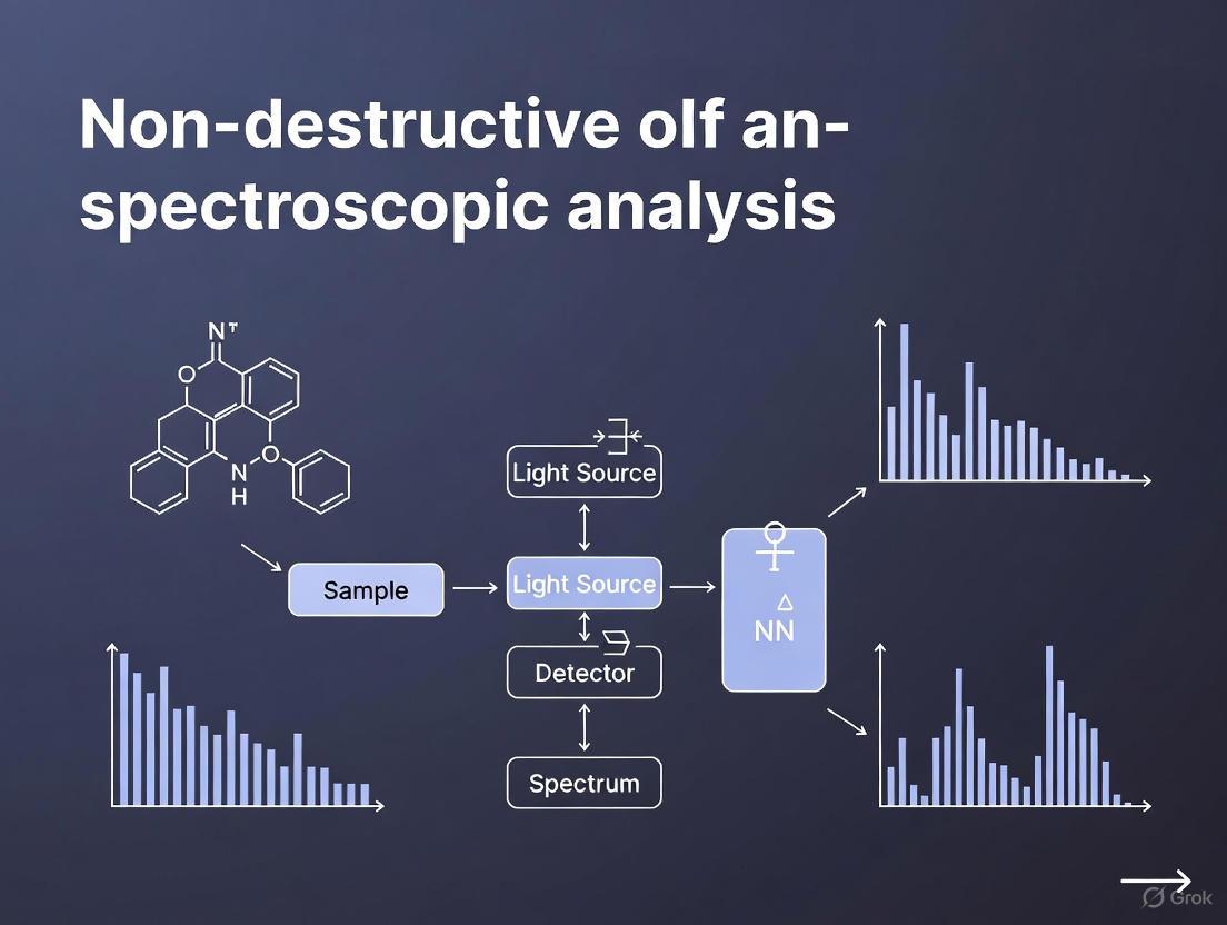
The following diagram illustrates the core workflow of a spectroscopic analysis, from measurement to result, highlighting the integrated nature of hardware, data processing, and model application.

Pharmaceutical Quality Control via NIR Spectroscopy

In-line Monitoring of Drug Products

In the pharmaceutical industry, NIR spectroscopy has been successfully implemented for the non-destructive quality control of final drug products, such as tablets. A key application involves using a specially designed multipoint measurement probe installed on a conveyor belt system to control both the distribution and content of the active pharmaceutical ingredient (API) across a production lot [34]. This approach overcomes limitations related to acquisition speed and sampling area, providing comprehensive physical and chemical knowledge of the product. The spatial and spectral information gathered serves as an innovative paradigm for real-time release strategy, a core objective of Process Analytical Technology (PAT) initiatives [34].

Detailed Experimental Protocol: Tablet Analysis on a Conveyor Belt

The following workflow details the methodology for in-line tablet monitoring:

• Instrumentation Setup: A Fourier Transform NIR (FT-NIR) spectrometer is coupled with a custom-designed fiber optic probe featuring multiple collection fibers. This probe is mounted above a conveyor belt transporting the tablets.
• Spectral Acquisition: The NIR probe scans each tablet as it passes on the conveyor belt. The system operates in reflectance mode, where the diffusely reflected light from the solid tablet is collected and sent to the detector [34] [32].
• Data Pre-processing: Acquired raw spectra are subjected to pre-processing techniques such as Standard Normal Variate (SNV) or Multiplicative Scatter Correction (MSC) to reduce the effects of light scattering and physical variations between tablets.
• Quantitative Modeling: A Partial Least Squares (PLS) regression model is used. This model, developed during the calibration phase, correlates the spectral variations with known variations in the API concentration (as determined by a reference method like HPLC).
• Prediction and Control: The calibrated PLS model is applied to the real-time spectral data from the production line to predict the API content in each tablet. The spatial data from the multipoint probe allows for monitoring the uniformity of API distribution across the batch.

Table 1: Key Performance Metrics in Pharmaceutical NIR Applications

Application Focus	Key Measured Variable	Sampling Mode	Primary Chemometric Method	Key Benefit
Tablet API Content [34]	Active Pharmaceutical Ingredient (API) Concentration	Reflectance	Partial Least Squares (PLS)	Real-time content uniformity analysis
Tablet API Distribution [34]	Spatial API Distribution	Multipoint Reflectance	Multipoint PLS Modeling	Ensures blend homogeneity
Process Analysis [32]	Component Concentration in Reactors	Fiber Optic Transflectance	PLS	In-line monitoring for process control

Non-Destructive Metabolite Estimation in Agricultural Products

Metabolite Profiling in Fresh Tea Leaves

NIR spectroscopy combined with machine learning has demonstrated significant potential for the non-destructive estimation of quality-related metabolites in fresh tea leaves (Camellia sinensis L.). Research has effectively estimated the contents of free amino acids (e.g., theanine), catechins, and caffeine using visible to short-wave infrared (400–2500 nm) hyperspectral reflectance data [31]. This approach addresses a critical need in tea cultivation and breeding, where traditional methods like High-Performance Liquid Chromatography (HPLC) are destructive, time-consuming, and expensive [31].

Detailed Experimental Protocol: Tea Leaf Metabolite Estimation

• Sample Preparation: Approximately 200 fresh tea leaves with varying status (e.g., different nitrogen conditions, leaf stages, shading conditions) are collected. Leaves are presented for scanning without destructive pre-treatment.
• Hyperspectral Data Acquisition: Reflectance spectra are acquired from each leaf at 1-nm intervals across the 400–2500 nm wavelength range using a hyperspectral sensor.
• Reference Analysis: The same scanned leaves are destructively analyzed post-scanning using HPLC to determine the precise concentrations of 15 metabolites, including catechins, caffeine, and free amino acids, creating the reference dataset for model training [31].
• Data Pre-processing and Modeling: Six spectral patterns are tested (Original Reflectance, First Derivative, etc.) with five machine learning algorithms (Random Forest, Cubist, etc.). The combination of De-trending (DT) pre-processing and the Cubist algorithm was robustly selected as the best-performing model for most metabolites over 100 repetitions [31].
• Model Validation: Model performance is evaluated using the Ratio of Performance to Deviation (RPD). Values above 1.4 are considered acceptable, and above 2.0 are considered accurate for analytical applications [31].

Table 2: Performance of NIR Spectroscopy in Estimating Tea Metabolites (Best Model: DT-Cubist) [31]

Metabolite	Mean RPD Value	Interpretation	Concentration Range (μg cm⁻²)
Total Catechins	2.7	Accurate Estimation	206.2 – 2528.7
(-)-Epigallocatechin Gallate (EGCG)	2.4	Accurate Estimation	91.0 – 619.8
Total Free Amino Acids	2.3	Accurate Estimation	12.3 – 746.0
Caffeine	1.8	Acceptable to Accurate	1.8 – 393.1
Theanine	1.5	Acceptable Estimation	0.2 – 264.5
Aspartate	2.5	Accurate Estimation	1.6 – 59.3

Protein Estimation in Rice Breeding

A similar NIRS approach is used in rice breeding programs for the rapid, non-destructive estimation of protein content in brown rice flour. This application is a case study in high-throughput phenotyping, essential for matching the efficiency of modern genotyping. Proteins contain chemical bonds (C-H, N-H) easily detected by NIRS, making this a suitable target [33]. The method involves scanning ground flour in a reflectance cup, followed by calibration using PLS regression against the reference protein data obtained via the Kjeldahl method or similar [33]. This allows breeders to screen early-generation material efficiently for a trait that influences cooking and eating quality.

Essential Reagents and Research Tools

The successful implementation of vibrational spectroscopy methods relies on a suite of specialized reagents and tools. The following table details the core components of the "Scientist's Toolkit" for these applications.

Table 3: Research Reagent Solutions for Vibrational Spectroscopy

Item / Solution	Function / Application	Key Consideration
FT-NIR Spectrometer [32]	Core instrument for acquiring high-resolution, wavelength-accurate spectra.	Superior stability and repeatability vs. dispersive systems; no software standardization needed between instruments.
Fiber Optic Reflection Probe [34] [32]	Enables in-line measurement on conveyor belts, in reactors, or hoppers.	Often engineered with automatic cleaning (e.g., high-pressure air) for process environments.
Hyperspectral Imaging Sensor [31]	Captures spatial and spectral information for heterogeneous solid samples like leaves.	Covers VIS-NIR-SWIR range (400-2500 nm) for broad metabolite estimation.
Chemometric Software (PLS, Cubist) [31] [32]	Develops calibration models linking spectral data to reference analytical results.	Machine learning algorithms (e.g., Cubist) can improve model accuracy for complex traits.
Calibration Standards [32]	A set of samples with known chemical values for building the quantitative model.	Must include all chemical, physical, and sampling variation the model will encounter; often requires 10x the number of components as a minimum.

Integrated Workflow from Sample to Result

The application of vibrational spectroscopy, whether in a laboratory or an industrial setting, follows a logical and integrated sequence. The diagram below maps the critical decision points and steps in the method development and deployment process, highlighting the non-destructive feedback loop that enables real-time control.

Vibrational spectroscopy, particularly NIR and IR, has firmly established itself as a powerful, non-destructive cornerstone for quality control and metabolite estimation. Its ability to provide rapid, non-invasive, and multi-parameter analyses aligns perfectly with the demands of modern industrial processes and advanced scientific research. The detailed protocols and performance data presented confirm that these techniques are not merely supplementary but are often the optimal choice for ensuring product quality in pharmaceuticals and accelerating phenotyping in agriculture. As spectroscopic instrumentation and machine learning algorithms continue to advance, the scope and accuracy of these non-destructive analyses are poised to expand further, solidifying their role as indispensable tools in the scientist's arsenal.

NMR Spectroscopy for Detailed Structural Elucidation of Complex Molecules

Nuclear Magnetic Resonance (NMR) spectroscopy stands as a cornerstone analytical technique in modern research for determining the complete structural composition of organic compounds and biomolecules. As a non-destructive method, it enables the detailed analysis of precious samples without consumption or alteration, preserving material for subsequent studies [35]. This whitepaper examines the fundamental principles, advanced methodologies, and practical applications of NMR spectroscopy, with particular emphasis on its growing role in pharmaceutical research and drug discovery where molecular complexity demands atomic-level precision.

The technique exploits the magnetic properties of certain atomic nuclei, which absorb and re-emit electromagnetic radiation at characteristic frequencies when placed in a strong magnetic field [36]. By measuring these frequencies, NMR provides detailed information about the electronic environment surrounding nuclei, revealing the number and types of atoms in a molecule, their connectivity, and their spatial arrangement [37]. This information is obtained from various NMR parameters including chemical shifts, coupling constants, and signal intensities, allowing scientists to construct a comprehensive picture of molecular structure and dynamics [37].

Fundamental Principles of NMR Spectroscopy

Theoretical Foundation

NMR spectroscopy originates from the intrinsic property of certain atomic nuclei possessing spin, characterized by the spin quantum number (I) [36]. Elements with either odd mass or odd atomic numbers exhibit nuclear "spin" [36]. For NMR-active nuclei such as hydrogen-1 (¹H) and carbon-13 (¹³C), the spin quantum number I = ½, resulting in two possible spin states (+½ and -½) [38]. In the absence of an external magnetic field, these states are energetically degenerate. However, when placed in a strong external magnetic field (B₀), this degeneracy is lifted, creating distinct energy levels through Zeeman splitting [36] [38].

The energy difference between these states corresponds to electromagnetic radiation in the radiofrequency region (typically 4-900 MHz) [36]. The precise resonance frequency of a nucleus depends on the strength of the applied magnetic field and its magnetogyric ratio (γ), a fundamental constant unique to each nuclide [36]. Crucially, the local electronic environment surrounding each nucleus slightly shields it from the applied field, causing subtle shifts in resonance frequency that form the basis of NMR's analytical power.

Key NMR Parameters for Structural Elucidation

NMR spectra contain rich information through several measurable parameters, detailed in the table below.

Table 1: Key Information Contained in NMR Spectra

Observable	Name	Quantitative Information	Structural Significance
Peak Position	Chemical Shift (δ)	δ(ppm) = (νobs - νref)/ν_ref	Chemical (electronic) environment of nucleus
Peak Splitting	Coupling Constant (J)	Peak separation (Hz)	Neighboring nuclei (torsion angles)
Peak Intensity	Integral	Relative height (ratio)	Nuclear count (ratio)
Peak Shape	Line Width	Δν = 1/πT₂	Molecular motion, chemical exchange

Chemical shift represents the resonance frequency of a nucleus relative to a standard reference compound (typically tetramethylsilane, TMS, set at 0 ppm) [39]. Expressed in parts per million (ppm), this parameter is independent of the instrument's magnetic field strength, allowing direct comparison of spectra acquired on different systems [39]. The chemical shift value indicates the electronic environment of the nucleus: shielded nuclei in electron-dense regions appear at lower δ values (upfield), while deshielded nuclei affected by electronegative atoms or π-systems appear at higher δ values (downfield) [39].

Spin-spin coupling occurs through bonds via the interaction between neighboring non-equivalent nuclei, causing splitting of NMR signals into multiplets [36]. The multiplicity follows the n+1 rule, where a proton with n equivalent neighboring protons displays a signal split into n+1 peaks [36]. The separation between these peaks is the coupling constant (J), expressed in Hz, which provides information about molecular geometry and stereochemical relationships [39].

Integration of signal areas provides quantitative information about the relative number of nuclei contributing to each signal, enabling determination of proton ratios within the molecule [39].

Experimental Methodologies and NMR Techniques

NMR Instrumentation and Workflow

A basic NMR spectrometer consists of several key components: a powerful magnet generating a stable, homogeneous magnetic field; a radiofrequency transmitter producing short, powerful pulses; a probehead containing the sample; a receiver coil detecting emitted radiofrequencies; and a computer system for data processing and analysis [36]. Modern Fourier-transform NMR (FT-NMR) instruments employ pulse sequences followed by mathematical transformation of the time-domain signal (free induction decay) into the familiar frequency-domain spectrum [39].

The experimental workflow begins with sample preparation, typically involving dissolution of the compound in a deuterated solvent (e.g., CDCl₃, D₂O, DMSO-d₆) to provide a lock signal and minimize interfering proton signals [36]. After sample insertion into the magnet, the instrument is tuned, shimmed to optimize magnetic field homogeneity, and calibrated before data acquisition. Subsequent processing includes Fourier transformation, phase correction, baseline correction, and referencing before spectral analysis.

Multi-Dimensional NMR Techniques

While 1D NMR (¹H and ¹³C) provides fundamental structural information, complex molecular structures often require advanced 2D NMR techniques that correlate nuclei through chemical bonds or through space.

Table 2: Common 2D NMR Experiments and Their Applications

Experiment	Type	Correlation	Structural Information
COSY	Homonuclear	¹H-¹H through bonds (2-3 bonds)	Proton-proton connectivity networks
HSQC/HMQC	Heteronuclear	¹H-¹³C through one bond	Direct proton-carbon connectivity
HMBC	Heteronuclear	¹H-¹³C through multiple bonds (2-3)	Long-range proton-carbon connectivity
NOESY/ROESY	Homonuclear	¹H-¹H through space (<5 Å)	Spatial proximity, stereochemistry
TOCSY	Homonuclear	¹H-¹H throughout spin system	All protons within coupled network

The following diagram illustrates a generalized workflow for structure elucidation using multi-dimensional NMR experiments:

Step-by-Step Protocol for NMR Structure Elucidation

Sample Preparation Protocol:

• Weighing: Transfer 2-10 mg of compound into a clean NMR tube [36]
• Solvation: Add 0.6-0.7 mL of deuterated solvent (CDCl₃, DMSO-d₆, etc.)
• Mixing: Cap and invert several times to ensure complete dissolution
• Labeling: Clearly label tube with compound identifier
• Loading: Insert tube into NMR spectrometer

Data Acquisition Protocol:

• Lock and Shim: Engage deuterium lock and optimize magnetic field homogeneity
• Tuning: Match and tune probe to sample
• Pulse Calibration: Determine 90° pulse width for quantitative conditions
• Spectral Width: Set to encompass all expected signals (0-14 ppm for ¹H)
• Acquisition Time: Typically 2-4 seconds for ¹H NMR
• Relaxation Delay: 1-5 seconds between scans for complete relaxation
• Scans: Collect 16-64 scans for ¹H; 1024+ scans for ¹³C NMR
• Processing: Apply Fourier transformation, phase correction, and baseline correction

Spectral Interpretation Protocol for ¹H NMR:

• Identify Solvent and Water Peaks: Recognize residual solvent signals
• Count Signals: Determine number of chemically distinct proton environments
• Integrate Peaks: Measure relative proton ratios from integration curves
• Analyze Chemical Shifts: Assign electronic environments using shift tables
• Determine Multiplicity: Apply n+1 rule to identify neighboring protons
• Measure J-Couplings: Extract coupling constants from multiplet patterns
• Correlate with 2D Data: Confirm assignments through COSY, HSQC, HMBC

For ¹³C NMR interpretation:

• Count Signals: Identify number of unique carbon environments
• Analyze Chemical Shifts: Assign carbon types (alkyl, aromatic, carbonyl, etc.)
• DEPT Experiments: Differentiate CH₃, CHâ‚‚, CH, and quaternary carbons
• Correlate with HSQC/HMBC: Connect carbon and proton networks

Advanced Applications in Drug Discovery and Development

NMR in Pharmaceutical Research

NMR spectroscopy has become indispensable in pharmaceutical research, particularly as drug molecules increase in complexity. The technique provides critical structural validation throughout the drug development pipeline, from initial discovery to regulatory submission [35]. In 2025, pharmaceutical companies are increasingly investing in NMR structure elucidation services to support ICH Q3A/B compliance and avoid regulatory observations related to unknown impurities [35].

Fragment-Based Drug Discovery (FBDD) represents a particularly powerful application of NMR, where screening libraries of low-molecular-weight compounds against target proteins identifies initial hits that can be optimized into potent drug candidates [37]. NMR's ability to provide detailed information on binding interactions at the atomic level makes it ideal for this purpose, enabling researchers to understand not just whether a compound binds, but how it binds [37].

A recent perspective published in the Journal of Medicinal Chemistry highlights the significant advancements and future potential of NMR-derived methods in drug discovery, emphasizing the technique's versatility throughout the development process [37]. The integration of cryoprobes and advanced pulse sequences has significantly improved the efficiency and accuracy of NMR measurements, enabling researchers to obtain high-quality data in less time [37].

Comparison with Other Structural Techniques

NMR provides complementary information to other structural biology techniques such as X-ray crystallography and cryo-electron microscopy (cryo-EM). The table below compares these primary methods for molecular structure determination.

Table 3: Comparison of Structural Determination Techniques in Drug Discovery

Parameter	NMR Spectroscopy	X-ray Crystallography	Cryo-Electron Microscopy
Sample State	Solution (native-like)	Crystal	Frozen hydrated
Sample Requirements	~0.5-1.0 mM, 250-500 μL	High-quality crystals	Low concentration (~0.01-0.1 mg/mL)
Molecular Weight Range	≤ ~50 kDa (routine)	No upper limit	> ~50 kDa
Hydrogen Atom Detection	Excellent	Poor	Poor
Dynamic Information	Excellent (timescales ps-s)	Limited	Limited
Time Requirements	Days to weeks	Days to months	Weeks to months
Key Limitations	Sensitivity, molecular weight	Crystallization, static snapshot	Resolution, sample preparation

Unlike X-ray crystallography, which provides a single static snapshot of a molecular structure, NMR captures the dynamic behavior of ligand-protein complexes in solution, revealing multiple conformational states and binding modes [40]. This is particularly valuable for understanding the subtle interplay between enthalpy and entropy critical for binding affinity and specificity [40]. Additionally, NMR can detect approximately 20% more protein-bound water molecules than X-ray crystallography, providing crucial information about hydration networks that mediate protein-ligand interactions [40].

Research Reagent Solutions

Table 4: Essential Materials for NMR Experiments

Item	Function	Application Notes
Deuterated Solvents (CDCl₃, DMSO-d₆, D₂O, etc.)	Provides signal for field frequency lock; minimizes interfering proton signals	Choice depends on sample solubility; store under inert atmosphere to prevent contamination
NMR Tubes	Holds sample within magnetic field; precision ensures spectral quality	Use matched tubes for best results; 5-7" length, 0.3 cm diameter standard [36]
Reference Standards (TMS, DSS)	Provides chemical shift reference point (0 ppm)	Added directly to sample or contained in capillary for external reference
Shift Reagents	Induces spectral changes for chiral analysis	Useful for determining enantiomeric purity and absolute configuration
NMR Software (Mnova, NMRium, TopSpin)	Processing, analysis, and visualization of NMR data	Enables peak picking, integration, multiplet analysis, and structure verification [41] [42]

Current NMR Methodologies in Drug Discovery

Recent advances in NMR technology have enhanced its utility in drug discovery. High-field NMR spectrometers (up to 1.2 GHz) provide unprecedented resolution and sensitivity, allowing for detailed analysis of large biomolecules and their interactions with potential drug candidates [37]. Paramagnetic NMR spectroscopy has emerged as a powerful technique to study protein-ligand interactions, leveraging the paramagnetic properties of certain metal ions to enhance NMR signals of nearby nuclei and provide valuable insights into spatial arrangements within complexes [37].

A novel research strategy termed NMR-Driven Structure-Based Drug Design (NMR-SBDD) combines a catalogue of ¹³C amino acid precursors, ¹³C side chain protein labeling strategies, and straightforward NMR spectroscopic approaches with advanced computational tools to generate protein-ligand ensembles [40]. This approach provides reliable and accurate structural information about protein-ligand complexes that closely resembles the native state distribution in solution [40].

The following diagram illustrates the integrated NMR-SBDD workflow for modern drug discovery:

NMR spectroscopy remains an indispensable tool for detailed structural elucidation of complex molecules, combining comprehensive analytical capabilities with non-destructive sample analysis. As technological advancements continue to address historical limitations in sensitivity and molecular weight range, NMR's applications in pharmaceutical research and drug discovery continue to expand. The integration of NMR with complementary structural biology techniques and computational methods creates a powerful synergistic approach for understanding molecular structure and function at atomic resolution, paving the way for the next generation of therapeutic agents and materials science innovations.

Hyperspectral Imaging and Machine Learning for Rapid, Non-Destructive Contaminant Detection

Hyperspectral imaging (HSI) represents a transformative analytical methodology that integrates conventional imaging and spectroscopy to simultaneously capture spatial and spectral information. This synergy creates a powerful framework for the non-destructive detection and identification of contaminants across diverse sectors, including pharmaceuticals, agriculture, and environmental monitoring. This technical guide elucidates the core principles of HSI, details the machine learning (ML) architectures that enable rapid analysis, and provides explicit experimental protocols validated in recent research. By providing a detailed roadmap from data acquisition to model interpretation, this whitepaper aims to equip researchers and drug development professionals with the knowledge to implement HSI-based contaminant detection, thereby upholding the critical principle of non-destructive analysis in spectroscopic research.

Hyperspectral imaging (HSI) is an advanced analytical technique that generates a three-dimensional data cube, or hypercube, comprising two spatial dimensions (x, y) and one spectral dimension (λ). Unlike traditional RGB imaging, which captures only three broad color bands (red, green, blue), HSI collects intensity data across hundreds of narrow, contiguous wavelength bands, generating a continuous spectrum for each pixel in an image [43]. This detailed spectral data acts as a unique "fingerprint" that can reveal the chemical composition and physical structure of a sample without causing any damage or alteration—a core tenet of non-destructive analysis [43].

The non-destructive nature of HSI makes it particularly valuable for applications where sample preservation is paramount. In pharmaceutical quality assurance, it allows for the verification of raw materials and finished products without compromising their integrity [44]. In food safety and agriculture, it enables the continuous monitoring of perishable goods for microbial or chemical contamination throughout the supply chain [45] [46]. The technology operates on the principle that when light interacts with a material, specific wavelengths are absorbed or reflected based on its molecular composition. By analyzing these subtle spectral variations, HSI can detect contaminants even before they become visually apparent, facilitating proactive intervention and ensuring product safety and quality.

Technical Foundations: From Data Acquisition to Machine Learning

The Hyperspectral Data Cube

A hyperspectral image is a complex dataset known as a hypercube. This structure can be visualized in two primary ways:

• Spatial View: A stack of images, each representing the same spatial area at a different wavelength.
• Spectral View: A collection of spectra, each representing the light intensity across all wavelengths for a single pixel.

The key advantage of this structure is the ability to perform spectral-spatial analysis. Researchers can identify the geographic location of a specific contaminant (spatial analysis) and simultaneously determine its chemical identity based on its spectral signature [47] [43].

Core System Components and Research Toolkit

A typical HSI system consists of several integrated hardware and software components. The table below details the essential elements of a research-grade HSI setup.

Table 1: Research Reagent Solutions: Essential Components of a Hyperspectral Imaging System

Component Category	Specific Examples & Specifications	Function in the Workflow
Imaging Sensors & Cameras	Visible Near-Infrared Camera (e.g., IMPERX 1920 × 1080), Short-Wave Infrared Camera (e.g., Guohui 640 × 512), CCD or CMOS sensors [47] [43].	Captures raw spatial and spectral data from the sample. Different cameras are optimized for specific spectral ranges (e.g., UV, VIS-NIR, SWIR).
Spectrograph & Lenses	Grating splitter; Lenses (e.g., Kowa 35 mm, AZURE 50 mm) [47].	Splits incoming light into its constituent wavelengths and focuses it onto the camera sensor.
Illumination	Halogen light sources; Dual-light source setups [47].	Provides consistent, uniform illumination across the sample to ensure reproducible spectral measurements.
Sample Handling	Motorized electric translation stages [47].	Moves the sample or sensor with precision for consistent scanning, especially in push-broom systems.
Calibration Standards	White reference tile (e.g., Spectralon), dark reference [47].	Critical for correcting raw images for sensor dark current and non-uniform light source intensity, converting data to reflectance.
Data Processing Software	ENVI, Python with scikit-learn, TensorFlow/PyTorch, custom chemometric tools [47] [45] [48].	Used for image calibration, preprocessing, feature extraction, and building machine learning models.
C13H17ClN4O	C13H17ClN4O, MF:C13H17ClN4O, MW:280.75 g/mol	Chemical Reagent
Practolol-d7	Practolol-d7, MF:C14H22N2O3, MW:273.38 g/mol	Chemical Reagent

Machine Learning for Spectral Analysis

The high dimensionality of HSI data makes machine learning and deep learning indispensable for its analysis. These algorithms automate the extraction of meaningful patterns and create predictive models for contaminant identification and quantification.

• Convolutional Neural Networks (CNNs): Modern research employs enhanced CNN architectures like CA-DSC-CNN (Channel Attention and Depthwise Separable Convolution CNN), which efficiently model spectral-spatial features while reducing computational complexity, achieving high correlation coefficients (R² > 0.89) in contamination prediction [45].
• Ensemble and Traditional Models: For many applications, ensemble models like XGBoost have proven highly effective, offering a strong balance between accuracy and robustness [48]. Traditional chemometric models such as Partial Least Squares Regression (PLSR) and Support Vector Machines (SVM) remain widely used for their interpretability and performance [46].
• Dimensionality Reduction: Techniques like the Successive Projections Algorithm (SPA) and Principal Component Analysis (PCA) are crucial for identifying the most informative wavelengths, thereby simplifying the model and mitigating the "curse of dimensionality" [46] [49].

Quantitative Performance: A Comparative Analysis of Applications

The efficacy of HSI and ML for contaminant detection is demonstrated by its performance across diverse fields. The following table summarizes quantitative results from recent, high-impact studies.

Table 2: Quantitative Performance of HSI & ML in Contaminant Detection Across Sectors

Application Domain	Target Contaminant / Defect	Optimal Model(s) Identified	Reported Performance Metrics
Food Safety (Eggs)	Microbial contamination (Aerobic Plate Count)	VIP-CA-DSC-CNN (Enhanced CNN with channel attention) [45]	Râ‚‚ = 0.8959, RMSE = 0.2396 [45]
Agriculture (Potatoes)	External defects (scab, mechanical damage)	SG-SNV preprocessing with K-Nearest Neighbors (KNN) model [46]	Detection accuracy: 83-93% for various defect types [46]
Environmental (Soil)	Hydrocarbons (crude oil, diesel)	XGB Regressor [48]	Râ‚‚ = 0.96, RMSE = 600 mg/kg [48]
Pharmaceuticals (TCM*)	Quality of Ganoderma lucidum (polysaccharides, ergosterol)	Genetic Algorithm-Optimized Extreme Learning Machine (GA-ELM) [47]	Râ‚‚ = 0.96 - 0.97 for component prediction [47]
Clinical Microbiology	Bacterial species (E. coli, Staphylococcus, etc.)	PCA-Discriminant Analysis (PCA-DA) on UV-HSI data [49]	90% classification accuracy [49]

TCM: Traditional Chinese Medicine

Detailed Experimental Protocols

To ensure reproducibility and provide a clear technical roadmap, this section outlines standardized experimental protocols derived from the cited research.

Protocol A: Detection of Microbial Contamination on Solid Surfaces

Based on the non-destructive detection of microbial contamination on eggshells [45].

• Sample Preparation:

  • Obtain a representative set of samples (e.g., 108 eggs).
  • Ensure sample surfaces are free of obvious physical debris that could interfere with imaging.

• Hyperspectral Image Acquisition:

  • Use a Visible-NIR (450-1100 nm) push-broom HSI system.
  • Acquire calibration images: a dark reference (with lens covered) and a white reference (using a standard Spectralon tile).
  • Scan each sample under consistent illumination and camera settings.
  • Convert raw images to reflectance using the formula: R = (I_raw - I_dark) / (I_white - I_dark) [47].

• Spectral Data Extraction & Preprocessing:

  • Use software (e.g., ENVI) to define Regions of Interest (ROIs) on each sample.
  • Extract the average spectrum from each ROI.
  • Preprocess the spectral data using algorithms like Savitzky-Golay (SG) smoothing to reduce noise and Standard Normal Variate (SNV) to correct for scatter.

• Feature Wavelength Selection:

  • Apply variable selection methods such as Variable Importance in Projection (VIP) or Competitive Adaptive Reweighted Sampling (CARS) to identify the most informative wavelengths and reduce data dimensionality.

• Model Development & Validation:

  • Partition the data into training and testing sets (e.g., 70/30 or 80/20 split).
  • Develop a Channel Attention and Depthwise Separable Convolution CNN (CA-DSC-CNN).
  • Train the model on the training set using the feature wavelengths as input and the reference microbial counts (e.g., from aerobic plate counts) as the target variable.
  • Validate the model on the held-out test set, reporting performance metrics like R² and RMSE.

Protocol B: Quantitative Analysis of Chemical Contaminants in Powders and Solids

Based on the quantitative evaluation of hydrocarbons in soil [48] and the analysis of Ganoderma lucidum [47].

• Sample Preparation:

  • Prepare samples with a known, wide range of contaminant concentrations (e.g., 0-10,000 mg/kg for hydrocarbons [48]).
  • For heterogeneous samples like medicinal powders, homogenize and press into a consistent form (e.g., coin-sized shapes on A4 paper) to ensure uniform imaging [47].

• Reference Analysis:

  • For each sample, determine the precise concentration of the target contaminant or component using a reference laboratory method (e.g., Gas Chromatography-Mass Spectrometry (GC-MS) for hydrocarbons [48] or High-Performance Liquid Chromatography (HPLC) for ergosterol [47]).

• Hyperspectral Image Acquisition & Calibration:

  • Acquire HSI data in the appropriate spectral range (e.g., SWIR for hydrocarbons, VIS-NIR for organic compounds).
  • Perform the same dark and white reference calibration as in Protocol A.

• Data Preprocessing & Dimensionality Reduction:

  • Preprocess spectra using Multiplicative Scatter Correction (MSC) or Normalization.
  • Use Successive Projections Algorithm (SPA) or Principal Component Analysis (PCA) to extract characteristic wavelengths.

• Model Development & Validation:

  • Train multiple machine learning models, such as XGBoost, Support Vector Regression (SVR), and Artificial Neural Networks (ANNs), on the preprocessed spectral data and reference concentration values.
  • Use k-fold cross-validation to tune model hyperparameters.
  • Select the best model based on its performance on an independent test set, prioritizing R² and RMSE.

The following workflow diagram synthesizes these protocols into a universal framework for HSI-based contaminant detection.

Diagram 1: Universal workflow for HSI-based contaminant detection and analysis, integrating sample preparation, data processing, and machine learning.

Advanced Data Processing: From RGB to Hyperspectral Reconstruction

A significant technological advancement is the reconstruction of hyperspectral data from standard RGB images using deep learning. This approach addresses the high cost and complexity of traditional HSI systems by leveraging widely available, high-resolution RGB cameras [43].

The process involves training a deep neural network to learn the complex mapping between a 3-band RGB input and a high-dimensional spectral signature. Models are trained on large datasets of paired RGB and hyperspectral images. Once trained, the network can predict a full spectrum for each pixel in a new RGB image, effectively creating a hyperspectral data cube from a simple color image [43]. This technique, while still an area of active research, promises to make spectral analysis accessible for a broader range of applications, including field-based and point-of-care contaminant screening.

Diagram 2: Deep learning-based workflow for reconstructing hyperspectral data cubes from standard RGB images, enabling more accessible spectral analysis.

The integration of hyperspectral imaging with machine learning establishes a robust, non-destructive paradigm for contaminant detection that aligns with the core principles of modern spectroscopic analysis. The technical protocols and performance data detailed in this guide demonstrate that HSI can achieve high accuracy in identifying and quantifying microbial, chemical, and physical contaminants across the pharmaceutical, agricultural, and environmental sectors. As deep learning techniques continue to evolve, making the technology more accessible and powerful, HSI is poised to become an indispensable tool for researchers and professionals committed to ensuring safety, quality, and integrity through non-destructive means.

The demand for safe, high-quality, and minimally processed products in the pharmaceutical and food industries has intensified the need for analytical techniques capable of assessing critical quality attributes in real-time [50]. Traditional analytical approaches, such as microbiological assays and chromatographic methods, are often destructive, labor-intensive, and time-consuming, making them unsuitable for continuous monitoring [50]. In contrast, spectroscopic techniques offer non-destructive, rapid, and reagent-free analysis, preserving sample integrity and enabling immediate feedback for process control [50] [51]. The non-destructive nature of spectroscopic analysis allows for the continuous examination of materials without altering their composition or structure, which is paramount for at-line or inline monitoring in manufacturing and for analyzing invaluable samples, such as extraterrestrial materials [51]. This whitepaper explores the operational principles, applications, and implementation strategies of real-time spectroscopy, with a focus on Near-Infrared (NIR) spectroscopy, highlighting its transformative role in modern industrial processes.

Core Spectroscopic Technologies for Real-Time Monitoring

Several spectroscopic techniques have been adapted for process analytical technology (PAT), each with unique strengths. Among these, Near-Infrared (NIR) spectroscopy has emerged as a leading technology due to its versatility and suitability for inline deployment [50].

Near-Infrared (NIR) Spectroscopy

NIR spectroscopy is a vibrational technique that measures molecular overtone and combination bands in the 780–2500 nm range. These absorptions arise from bonds including C-H, N-H, and O-H, which are abundant in most organic materials, allowing for the rapid assessment of composition and structure [50]. The resulting spectra are broad and overlapping, necessitating chemometric methods for interpretation. Multivariate models like Principal Component Analysis (PCA) and Partial Least Squares Regression (PLSR) are employed to extract predictive information on parameters such as moisture content, protein levels, and microbial load [50]. Advances in miniaturization have led to portable and handheld NIR spectrometers, enabling real-time, non-invasive evaluations directly in production, storage, or retail environments [50].

Other Relevant Techniques

• Fourier Transform Infrared (FTIR) Spectroscopy: Often used in mid-infrared regions for detailed molecular "fingerprinting," with advanced techniques like nanoscale IR spectroscopy achieving sub-micron resolution for analyzing microscopic samples [51].
• Hyperspectral Reflectance Spectroscopy (HRS): Captures reflected radiation across hundreds of spectral channels in the optical spectrum (400–2500 nm), allowing for the creation of detailed spatial maps of chemical properties [52].
• Atomic Spectroscopy: Techniques like ICP-OES and AAS are highly sensitive for elemental analysis but are generally more suited for offline laboratory use due to their destructive nature and sample preparation requirements [53].

Table 1: Comparison of Spectroscopic Techniques for Process Monitoring

Technique	Typical Spectral Range	Key Measurable Parameters	Primary Strength	Suitability for Real-Time
NIR Spectroscopy	780–2500 nm	Moisture, Fat, Protein, API concentration	Rapid, non-destructive, deep penetration	Excellent (Inline/Online)
FTIR Spectroscopy	400–4000 cm⁻¹	Molecular functional groups, contaminants	Detailed chemical fingerprinting	Good (At-line/Inline)
Hyperspectral Imaging	400–2500 nm	Spatial distribution of composition	Combines imaging and spectroscopy	Good (At-line/Inline)
ICP-OES	166–847 nm	Elemental composition, trace metals	High sensitivity for multi-element analysis	Poor (Offline)

Experimental Protocols and Methodologies

Implementing spectroscopy for real-time monitoring requires careful experimental design, from sample presentation to data analysis. The following protocols outline standard methodologies for different applications.

Protocol for NIR-Based Food Freshness Assessment

This protocol is adapted from studies monitoring spoilage in meat and seafood [50].

1. Objective: To predict microbial load and total volatile basic nitrogen (TVB-N) in meat samples non-destructively using a portable NIR spectrometer. 2. Materials and Reagents: * Portable NIR spectrometer (e.g., with a spectral range of 900–1700 nm) * Reflectance probe or sample cup for uniform presentation * Fresh meat samples (e.g., beef steaks, fish fillets) * Reference methods: Microbiological plating apparatus, TVB-N distillation unit 3. Procedure: * Sample Preparation: Cut samples into uniform sizes. For calibration, obtain samples with varying degrees of freshness (e.g., different storage days). * Spectral Acquisition: Place the sample against the reflectance probe or in the sample cup. Acquire NIR spectra with the following typical instrument settings: 64 scans per spectrum, resolution of 8–16 cm⁻¹. For each sample, collect spectra from at least three different spots to account for heterogeneity. * Reference Data Collection: Immediately after spectral acquisition, destructively analyze the same sample spots using standard microbiological methods (e.g., total plate count) and TVB-N analysis to obtain reference values. * Chemometric Modeling: * Data Pre-processing: Apply techniques like Standard Normal Variate (SNV) or Multiplicative Scatter Correction (MSC) to remove light-scattering effects. * Model Development: Use a calibration dataset to build a Partial Least Squares Regression (PLSR) model correlating the pre-processed NIR spectra with the reference values. * Model Validation: Validate the model using an independent set of samples not included in the calibration. Key performance metrics include Root Mean Square Error of Prediction (RMSEP) and Coefficient of Determination (R²). 4. Real-Time Implementation: Once validated, the model can be deployed on the portable spectrometer or an inline system to predict microbial load/TVB-N in new samples in seconds based on their NIR spectrum alone.

Protocol for Quality Assessment of Concrete via HRS

This protocol demonstrates the versatility of spectroscopy beyond pharmaceuticals and food, using HRS for non-destructive evaluation of construction materials [52].

1. Objective: To assess the microstructural quality and curing efficacy of high-strength concrete using Hyperspectral Reflectance Spectroscopy. 2. Materials and Reagents: * Portable spectroradiometer (operating in 400–2500 nm range) * Calibrated reference panel (e.g., coated with BaSO₄) * Concrete samples subjected to different curing regimes (e.g., internally cured, conventionally cured, non-cured) 3. Procedure: * Spectral Measurement Setup: The instrument parameters are set (e.g., integration time of 10 milliseconds, internal scans of 50). Measurements are acquired in a controlled laboratory environment [52]. * Calibration: A reference spectral measurement is acquired over the calibrated panel to convert raw data into absolute reflectance. * Data Acquisition: For each concrete sample, the spectral measurement is normalized by dividing it with the measurement from the reference panel. Multiple measurements per sample are recommended. * Data Analysis: * Qualitative Analysis: Visually inspect the spectral signatures for distinct absorption features, particularly at water absorption bands (e.g., 1150 nm, 1400 nm, 1900 nm). Well-cured, less porous concrete typically shows higher overall reflectance and subdued water absorption features [52]. * Quantitative Analysis: Develop a Concrete Quality Metric (CQM) based on derivative spectrometry or other spectral indices to numerically assess porosity and curing quality, correlating with destructive tests like sorptivity.

Implementation in Industrial Processes

Transitioning spectroscopy from the laboratory to the production floor involves strategic integration and an understanding of operational constraints.

Integration with Process Analytical Technology (PAT)

Process Analytical Technologies have been field-proven for nearly three decades. Fiber optic-based dispersive grating spectrometers have revolutionized process monitoring, offering high acquisition speed, a broad measurement range, and sensitivity [54]. For instance, a comprehensive dataset that would typically require hours of laboratory analysis can be captured in about a minute with a process spectrometer [54]. These systems are designed for durability, with some models operating continuously 24/7 for over 10 years with more than 99% uptime, ensuring long-term reliability with minimal maintenance compared to techniques like process gas chromatography [54].

Portable and Online Systems

The choice between portable and fixed online systems depends on the application need.

• Portable Handheld Spectrometers: Used for spot-checking and mapping quality in warehouses, receiving docks, or large equipment. For example, a handheld NIR spectrometer was used to classify Angus beef steaks by aging status with over 90% accuracy directly in a storage facility [50].
• Inline or Online Systems: Integrated directly into a continuous processing line, such as a conveyor belt or pipeline. Here, NIR probes and flow cells continuously monitor the product stream, sending data to a control system that can make real-time adjustments to process parameters (e.g., mixing speed, heating temperature) to maintain product quality [50].

The Scientist's Toolkit: Essential Research Reagent Solutions

The following table details key materials and reagents commonly used in developing and validating spectroscopic methods for process monitoring.

Table 2: Essential Materials and Reagents for Spectroscopic Process Monitoring

Item	Function/Description	Application Example
Chemometric Software	Software for multivariate calibration and model development (e.g., PLS, PCA).	Essential for building models to predict concentration or quality parameters from spectral data.
Calibration Reference Standards	Stable, well-characterized materials with known properties for instrument calibration and performance verification.	Ensuring measurement accuracy and transferability of models between instruments.
NIR Spectrometer	Instrument for acquiring spectra in the near-infrared region; can be benchtop, portable, or inline.	The primary tool for non-destructive, rapid data acquisition.
Polyethylene Glycol (PEG)	Used as an internal curing agent in material science; studied via HRS.	Model compound for evaluating microstructural refinement in concrete [52].
FTIR Spectrometer	Instrument for acquiring mid-infrared spectra, often with higher resolution than NIR.	Detailed molecular fingerprinting and identification of unknown contaminants.
Probe-Based Sampling Interface	Fiber optic probes (reflectance or transmittance) for analyzing samples in situ.	Enables direct analysis of powders, slurries, and liquids in reactors or pipes without sample withdrawal.
D-Phenylglycyl Cefaclor-d5	D-Phenylglycyl Cefaclor-d5, MF:C23H21ClN4O5S, MW:506.0 g/mol	Chemical Reagent
Lufenuron-13C6	Lufenuron-13C6, MF:C17H8Cl2F8N2O3, MW:517.10 g/mol	Chemical Reagent

The field of real-time spectroscopic monitoring is rapidly evolving, driven by advancements in hardware and data analytics. Emerging trends include the integration of Artificial Intelligence (AI) and deep learning algorithms, such as Convolutional Neural Networks (CNNs), to enhance the accuracy and robustness of chemometric models [50]. Furthermore, the fusion of spectroscopic data with other process information in IoT-linked platforms and cloud-based monitoring systems enables predictive analytics and full supply chain traceability [50]. The development of hybrid sensing systems, which combine the broad compositional assessment of NIR with the specificity of biosensors, represents the next frontier in comprehensive quality and safety assurance [50].

In conclusion, real-time process monitoring with spectroscopy represents a paradigm shift from off-line, destructive testing to integrated, non-destructive quality control. Techniques like NIR and HRS provide a powerful means to ensure product quality, optimize processes, and reduce waste across diverse industries, from drug manufacturing to food safety and beyond. Their non-destructive nature, combined with speed and the ability to provide deep chemical insight, makes them indispensable tools for modern researchers and industrial professionals striving for efficiency and excellence.

Optimizing Analytical Outcomes: Tackling Sample Preparation and Data Challenges

In the realm of analytical science, particularly within pharmaceutical development and non-destructive spectroscopic analysis, sample preparation represents the most critical link in the chain of analytical reliability. Errors introduced during this initial phase are not merely incidental; they are systematic errors that propagate through the entire analytical process, ultimately compromising data integrity, regulatory submissions, and patient safety [55]. While modern analytical instruments like spectrometers generate extensive "big data" sets, the value of this data is entirely dependent on the quality of the sample preparation that precedes it [56]. In non-destructive analysis, where samples cannot be altered, damaged, or consumed, proper preparation takes on even greater significance as it often represents the only opportunity to optimize the sample-analyst interaction.

This technical guide examines the pivotal role of sample preparation in mitigating up to 60% of analytical errors, framing this discussion within the context of non-destructive spectroscopic analysis. We will explore systematic approaches for different sample types, detailed experimental protocols, and the crucial connection between meticulous preparation and the reliability of subsequent non-destructive evaluation.

The Error Landscape in Analytical Chemistry

Classification and Impact of Analytical Errors

Analytical errors are broadly categorized as either random or systematic. Random errors arise from unpredictable variations in the measurement process and are often associated with instrumental noise. In contrast, systematic errors (or biases) result from consistent, predictable influences that skew results in a specific direction. Sample preparation errors fall squarely into the latter category, making them particularly pernicious as they cannot be eliminated through statistical averaging of repeated measurements [55].

The statement that sample preparation contributes to approximately 60% of analytical errors stems from the fact that sample preparation is often the most variable and operator-sensitive step in the analytical process. These errors directly impact the accuracy of calibration curves, lead to false positives or negatives in detection, and ultimately result in incorrect scientific conclusions or quality assessments.

Error Propagation in Non-Destructive Analysis

In non-destructive spectroscopic analysis, such as Fourier-transform infrared (FT-IR) spectroscopy or Raman spectroscopy, the analytical process is designed to preserve the sample. However, this does not eliminate the potential for preparation-related errors. For instance, improper handling can lead to:

• Surface contamination affecting reflectance measurements
• Inconsistent presentation geometry causing signal variation
• Environmental exposure altering sample chemistry before analysis
• Suboptimal substrate choice creating interfering background signals

The subsequent non-destructive measurement merely captures these prepared states, meaning any systematic error introduced during preparation becomes permanently embedded in the analytical record [57] [58].

Table 1: Classification of Sample Preparation Errors and Their Impacts

Error Category	Examples	Impact on Analysis	Common Mitigation Strategies
Weighing Errors	Incorrect mass measurement, hygroscopicity, static charge	Incorrect concentration calculations, calibration inaccuracies	Use of calibrated balances, anti-static devices, controlled environment [59]
Transfer & Contamination	Incomplete quantitative transfer, container interactions	Loss of analyte, introduction of interferents	Proper rinsing techniques, use of inert containers, method validation [55]
Extraction Inefficiency	Incomplete dissolution, inadequate extraction time	Underestimation of analyte concentration	Sonication optimization, solvent selection, shaking/vortexing [59]
Matrix Effects	Protein binding, chemical interference, pH variation	Altered analytical response, signal suppression/enhancement	Masking/chelating agents, pH adjustment, sample clean-up [55] [60]

Fundamental Sample Preparation Methodologies

Preparation of Solutions from Solid and Liquid Materials

The preparation of standard and sample solutions with accurate concentration is fundamental to quantitative analysis. The process differs significantly between solid and liquid starting materials.

Preparation from Solid Materials:

• Glassware Selection and Cleaning: Begin with appropriate Class A volumetric flasks cleaned thoroughly via an acid bath (1% HCl or HNO₃) with appropriate personal protective equipment, followed by soap and multiple rinses with distilled water [55].
• Weighing: Accurately weigh the required solid sample on an analytical balance rather than a standard top-loading balance for improved accuracy. For hygroscopic materials, pre-drying in an oven or desiccator may be necessary [55].
• Dissolution: Transfer the solid to a volumetric flask and add approximately ¾ of the final solvent volume. Swirl to dissolve completely before filling to the calibration mark. The meniscus should just touch the fill line. Invert the flask several times with the cap secured for thorough mixing [55].

Preparation from Liquid Materials:

• Volumetric Transfer: Use a transfer pipette filled to the calibration line using a pipette bulb. Deliver the liquid into a volumetric flask without blowing out the last drop [55].
• Dilution to Volume: Fill the volumetric flask to the calibration line so the meniscus touches the line, then mix by inverting several times [55].

Filtration Techniques for Particulate Removal

Filtration is employed to remove undissolved solids that might interfere with analysis or damage instrumentation. Several approaches are available:

• Filter Flask Setup: Place filter paper on a fritted glass filter attached to a filter flask. Apply vacuum to the flask arm, potentially with a trap to prevent liquid from entering the vacuum system. Pour the sample through the filter paper until a dry powder remains [55].
• Syringe Filtration: Add the sample to a clean syringe with a Luer lock end. Screw a syringe filter into the Luer lock, push the plunger, and collect the filtered liquid [55].
• Spin Filtration: Pre-rinse the filter with buffer or ultrapure water. Insert the spin filter into a microcentrifuge tube, load the sample on top, cap the tube, and centrifuge for 10-30 minutes (while properly balanced). The filtered solution collects in the bottom of the tube [55].

Masking and Chelating Techniques

For analyses involving metal ions, particularly in complex matrices, masking and chelating techniques are essential:

• pH Adjustment: Adjust the sample to an appropriate pH depending on the formation constants of the masking and chelating agents [55].
• Masking Agent Addition: Add the masking agent to the solution and allow it to react for at least 10 minutes with the target metal ion. This prevents unwanted metals from being detected [55].
• Chelation: Add the chelating reagent (e.g., EDTA, which typically forms a 1:1 complex with metal ions) in molar quantities equivalent to the metal to be chelated [55].
• Demasking: Add a chemical that reacts with the masked metal ion to release it for analysis or recovery by precipitation [55].

Sample Preparation Workflow for Non-Destructive Analysis

Advanced Preparation Techniques for Specific Applications

Pharmaceutical Sample Preparation

In regulated pharmaceutical testing, sample preparation follows meticulously designed and validated procedures to ensure accuracy, precision, and reproducibility.

Drug Substance (DS) Preparation: The "dilute and shoot" approach is commonly employed for drug substances, but requires careful execution:

• Weighing: Weigh 25-50 mg of DS reference standard or sample on a five-place analytical balance using folded weighing paper or a weighing boat to reduce spillage [59].
• Transfer and Solubilization: Quantitatively transfer all powders to an appropriately sized Class A volumetric flask. Add about ¾ of the diluent (selected based on API solubility and stability) and solubilize using sonication, shaking, or vortex mixing [59].
• Final Preparation: Add solvent to the calibration mark and mix thoroughly. Transfer an aliquot to an HPLC vial using a disposable pipette. Filtration of DS solutions is generally discouraged as drug substances should not contain particulate matter [59].

Drug Product (DP) Preparation: For solid dosage forms like tablets and capsules, a "grind, extract, and filter" approach is typically employed:

• Particle Size Reduction: Crush 10-20 tablets in a porcelain mortar and pestle, or use a hammer for single tablets wrapped in weighing paper [59].
• Quantitative Transfer: Transfer all particles quantitatively to a volumetric flask, rinsing to ensure complete transfer [59].
• Extraction: Add diluent and extract using optimized sonication, shaking, or vortexing to ensure complete API dissolution [59].
• Filtration: Filter the extract through a 25-mm 0.45 μm disposable syringe membrane filter (nylon or PTFE), discarding the first 0.5 mL of filtrate [59].

Preparation for Non-Destructive Spectroscopic Analysis

Non-destructive analysis presents unique sample preparation challenges, as the sample must remain unaltered for future analysis or preservation.

Cultural Heritage and Mineralogical Applications: In fields such as cultural heritage analysis, where samples cannot be powdered or disassembled, preparation focuses on optimal presentation:

• Surface Preparation: Gently remove loose debris without altering the surface chemistry using soft brushes or inert gases [57] [58].
• Stabilization: Secure samples in position without chemical adhesives that might interfere with spectroscopic readings [58].
• Environmental Control: Maintain consistent temperature and humidity during analysis to prevent spectral drift [57].

Modern Spectroscopic Data Preprocessing: While not sample preparation in the traditional sense, data preprocessing is essential for extracting meaningful information from non-destructive analyses:

• Mathematical Transformations: Apply affine transformations, min-max normalization, or Savitzky-Golay filtering to highlight spectral features while maintaining the integrity of the raw data [56].
• Noise Reduction: Implement smoothing processes to reduce the impact of instrumental noise while preserving critical spectral features [56].
• Dimensionality Reduction: Employ principal component analysis (PCA) or cluster analysis to manage the "big data" nature of spectroscopic datasets [56].

Table 2: Advanced Sample Preparation Techniques for Different Sample Types

Technique	Principle	Applications	Advantages	Limitations
Solid-Phase Extraction (SPE)	Partitioning of analytes between liquid sample and solid stationary phase [60]	Pharmaceutical bioanalysis, environmental samples	High enrichment factors, clean-up capability, automation potential	Possible breakthrough, cartridge variability, method development time
Solid-Phase Microextraction (SPME)	Equilibrium extraction using coated fiber [60]	Volatile/semivolatile compounds, in vivo analysis	Minimal solvent use, integration of sampling and extraction, portability	Fiber fragility, limited loading capacity, matrix effects
Liquid-Phase Microextraction (LPME)	Miniaturized solvent extraction in μL volumes [60]	Preconcentration of pharmaceuticals from biological fluids	High enrichment, low cost, simple operation	Difficult automation, relatively long extraction times
Microdialysis (MD)	Diffusion across semipermeable membrane [60]	In vivo sampling from brain, blood, tissues	Continuous monitoring, minimal tissue damage, protein-free samples	Low relative recovery, membrane fouling, surgical skill required

The Scientist's Toolkit: Essential Research Reagent Solutions

Table 3: Essential Materials and Reagents for Sample Preparation

Item	Function/Application	Key Considerations
Class A Volumetric Flasks	Precise volume measurement for standard and sample solutions [55]	Certification, cleanliness, proper meniscus reading
Analytical Balances	Accurate mass measurement of standards and samples [55]	Calibration, environmental controls, anti-static devices
Syringe Filters (0.45 μm, 0.2 μm)	Removal of particulate matter from samples [55] [59]	Membrane composition (nylon, PTFE), size, compatibility
Ultrasonic Baths	Enhancing dissolution through cavitation [55] [59]	Temperature control, optimization of sonication time
pH Adjustment Reagents	Optimizing chemical conditions for extraction or masking [55]	Buffer capacity, compatibility with analytes
Masking & Chelating Agents	Selective binding of interfering metal ions [55]	Formation constants, pH dependence, selectivity
SPME Fibers	Solvent-free extraction and concentration of volatiles [60]	Coating chemistry, thickness, conditioning requirements
Stability Chambers	Controlled environmental conditions for stability testing [61]	Temperature/humidity control, monitoring, calibration
Asoprisnil-d3	Asoprisnil-d3|Stable Labeled SPRM|	Asoprisnil-d3 is a stable isotope-labeled internal standard for research on selective progesterone receptor modulators (SPRMs). For Research Use Only.
Artemisinin-d4	Artemisinin-d4 Stable Isotope

Quality Assurance and Regulatory Considerations

Method Validation in Sample Preparation

The robustness of sample preparation methods must be systematically validated to ensure reliability, particularly in regulated environments like pharmaceutical quality control:

• Specificity: Demonstrate that the sample preparation procedure effectively isolates the target analytes from matrix components [62].
• Accuracy: Establish that the preparation method provides extraction efficiencies close to 100% through spike-recovery experiments [62].
• Precision: Verify that the procedure yields reproducible results across multiple preparations, operators, and days [62].
• Robustness: Validate that small, deliberate variations in preparation parameters (pH, extraction time, solvent composition) do not adversely affect results [62].

Stability Considerations

Sample stability must be assessed throughout the preparation and analysis workflow:

• Short-term Stability: Evaluate sample integrity during the preparation process itself [61].
• Processed Sample Stability: Determine how long prepared samples remain stable under analysis conditions [61].
• Storage Conditions: Establish appropriate storage conditions for both raw and prepared samples, potentially using stability chambers with programmable controls for temperature and humidity [61].

Error Mitigation Throughout the Analytical Process

Sample preparation is not merely a preliminary step in analytical workflows but a fundamental determinant of data quality and reliability. By recognizing that approximately 60% of analytical errors originate in this phase, researchers can allocate appropriate resources, training, and methodological rigor to this critical activity. In the context of non-destructive analysis, where samples remain available for future study, proper preparation takes on additional significance as it represents an investment in long-term analytical assets.

The systematic approaches outlined in this technical guide—from fundamental solution preparation to advanced microextraction techniques—provide a framework for minimizing systematic errors and maximizing analytical accuracy. By integrating these methodologies with appropriate quality assurance measures and a thorough understanding of error propagation, researchers across pharmaceutical development, materials characterization, and cultural heritage analysis can significantly enhance the reliability of their non-destructive spectroscopic analyses.

Within the framework of non-destructive spectroscopic research, sample preparation is a critical step that directly influences data accuracy, reliability, and analytical throughput. While techniques like X-ray Fluorescence (XRF) are inherently non-destructive, their accuracy is heavily dependent on proper sample presentation to minimize matrix effects. Conversely, techniques like Inductively Coupled Plasma Mass Spectrometry (ICP-MS) require sample digestion and introduction in liquid form, making dilution protocols paramount for success. This guide details the core best practices for pelletizing samples for XRF analysis and diluting them for ICP-MS, providing researchers and drug development professionals with standardized methodologies to ensure data integrity and regulatory compliance.

Fundamental Principles: XRF and ICP-MS at a Glance

X-Ray Fluorescence (XRF)

XRF is an analytical technique that determines the elemental composition of a material. It works by bombarding a sample with high-energy X-rays, causing the atoms within the sample to become excited and emit secondary (or fluorescent) X-rays. The energy of these emitted X-rays is characteristic of the elements present, allowing for their identification and quantification [63] [64]. A key advantage of XRF is its non-destructive nature, meaning the sample remains intact and can be used for further analysis after measurement [65] [63]. It is versatile and can analyze solids, liquids, and powders with minimal preparation.

Inductively Coupled Plasma Mass Spectrometry (ICP-MS)

ICP-MS is a powerful technique used for trace and ultra-trace multi-element analysis. The sample, typically in a liquid form, is nebulized into a fine aerosol and introduced into an argon plasma, which operates at temperatures high enough to atomize and ionize the elements. These ions are then separated and quantified based on their mass-to-charge ratio by a mass spectrometer [66]. ICP-MS is renowned for its exceptionally low detection limits, wide dynamic range, and high sample throughput [66] [67]. However, it is a destructive technique, as samples are consumed during the analysis.

Table 1: Core Characteristics of XRF and ICP-MS

Aspect	XRF (X-ray Fluorescence)	ICP-MS (Inductively Coupled Plasma Mass Spectrometry)
Analytical Principle	Measures characteristic fluorescent X-rays emitted from a sample [63].	Measures ions produced by high-temperature argon plasma [66].
Nature of Technique	Typically non-destructive [65] [63].	Destructive [65].
Sample Form	Solids, powders, liquids [65] [63].	Primarily liquid solutions [66] [68].
Key Strength	Rapid, minimal preparation, non-destructive.	Extremely low detection limits (ppt), high precision, multi-element capability [66] [67].
Typical Application	Quality control, raw material verification, contamination screening [65] [64].	Trace impurity testing, ultra-trace element quantification in pharmaceuticals [65] [66].

Pelletizing for XRF Analysis

The Rationale for Pelletizing

For the analysis of powdered samples—such as raw pharmaceutical ingredients or soil samples in environmental monitoring—creating a pressed pellet is a standard preparation method. This process ensures a homogeneous, flat, and consistent surface for X-ray irradiation, which is crucial for obtaining accurate and reproducible results. A well-prepared pellet minimizes particle size effects, enhances the uniformity of the analyzed volume, and reduces heterogeneity and surface imperfections that can scatter X-rays and introduce analytical errors.

Detailed Experimental Protocol for Pellet Preparation

The following workflow outlines the key steps for creating a high-quality pressed pellet for XRF analysis.

Step 1: Grinding and Homogenization The sample powder is first finely ground using a mill or mortar and pestle to achieve a consistent and small particle size (typically < 50 µm). This critical step breaks down agglomerates and ensures a homogeneous mixture, reducing mineralogical and particle size effects that can significantly affect X-ray intensity.

Step 2: Mixing with Binder The ground powder is then mixed with a binding agent (e.g., cellulose wax, boric acid) in a specific ratio, commonly 10:1 (sample to binder). The binder provides mechanical strength to the pellet, preventing it from crumbling during handling and analysis. Thorough mixing in a vortex mixer or similar device is essential for a uniform mixture.

Step 3: Loading into a Pellet Die The mixture is carefully transferred into a cylindrical pellet die, typically made of hardened steel. The die chamber must be clean and smooth to ensure easy ejection and a pellet with a flawless surface.

Step 4: Pressing in a Hydraulic Press The loaded die is placed in a hydraulic press. Pressure is applied gradually and held at a defined tonnage (commonly 10-25 tons for a 40-mm diameter pellet) for a set time (e.g., 30-60 seconds). This pressure compacts the powder-binder mixture into a solid, coherent pellet.

Step 5: Ejection and Storage After pressing, the pressure is released, and the pellet is carefully ejected from the die. The finished pellet should be stored in a desiccator to prevent moisture absorption, which could alter its XRF properties, until it is ready for analysis.

The Scientist's Toolkit: Key Reagents and Materials for XRF Pelletizing

Table 2: Essential Materials for XRF Pellet Preparation

Item	Function	Technical Notes
Hydraulic Press	Applies high, uniform pressure to compact powder into a solid pellet.	Capable of generating 10-25 tons of force.
Pellet Die	A cylindrical mold that defines the shape and size of the final pellet.	Typically made of hardened steel or tungsten carbide.
Binding Agent	Provides structural integrity to the pellet, preventing it from breaking.	Common binders: cellulose, boric acid, wax. Inert to avoid spectral interference.
Grinding Mill	Reduces particle size and ensures sample homogeneity.	Agate or tungsten carbide mills are preferred to avoid contamination.
Pellet Die Lubricant	Aids in the release of the pellet from the die after pressing.	Boric acid powder can be used as a releasing agent for the die walls.
Cy2 (iodine)	Cy2 (iodine), CAS:186205-37-8, MF:C25H27IN2O4, MW:546.4 g/mol	Chemical Reagent
CFTR corrector 3	CFTR Corrector 3 (VRT-325) For Research	CFTR Corrector 3 (VRT-325) is a small molecule for investigating F508del-CFTR trafficking. This product is For Research Use Only.

Dilution for ICP-MS Analysis

The Rationale for Dilution in ICP-MS

Dilution is a fundamental sample preparation step for ICP-MS to manage the total dissolved solids (TDS) content in the introduced solution. The widely accepted maximum TDS level for robust routine analysis is 0.2% (2000 ppm) [69] [70] [68]. Exceeding this limit can cause several issues:

• Matrix Deposition: High salt levels can build up on the interface cones (sampler and skimmer), leading to signal drift and instrument instability.
• Ionization Suppression: Easily ionized elements (e.g., Na, K, Ca) in the matrix can suppress the ionization of analytes, reducing sensitivity, particularly for poorly ionized elements like As, Cd, and Hg [69] [70].
• Spectral Interferences: A high matrix load can increase the formation of polyatomic ions that interfere with the measurement of target analytes.

Detailed Experimental Protocol for Sample Dilution

The workflow below outlines the primary steps for preparing a liquid sample for ICP-MS analysis, with a focus on dilution.

Step A: Determine Total Dissolved Solids (TDS) If the TDS of the original sample digest is unknown, it can be estimated gravimetrically by evaporating a known volume of the solution and weighing the residual solids. For many prepared samples, the TDS can be calculated based on the sample weight and final digest volume.

Step B: Calculate the Required Dilution Factor Based on the TDS, calculate the dilution factor required to bring the final TDS to ≤ 0.2%. For example, a soil digest with an estimated 2% TDS would require at least a 10-fold dilution (2% / 10 = 0.2%).

Step C: Perform the Dilution Dilute an aliquot of the sample digest using a high-purity diluent, typically a 1-2% nitric acid (HNO₃) solution. The acid matrix helps to stabilize the elements as ions in solution and prevents them from adsorbing to the walls of the container [68]. Use Class A volumetric glassware or calibrated automatic pipettes for accuracy. All labware must be scrupulously clean to avoid contamination.

Step D: Add Internal Standard(s) After dilution, add a known concentration of internal standard elements (e.g., Sc, Ge, Rh, In, Lu, Bi) to both the samples and calibration standards. Internal standards correct for instrument drift, matrix-induced signal suppression/enhancement, and variations in sample viscosity and nebulization efficiency [69] [68].

Step E: Analysis and Quality Control Analyze the diluted samples against a calibration curve prepared in the same acid matrix. Include quality control samples such as procedural blanks, certified reference materials (CRMs), and spike recovery samples to validate the accuracy and precision of the entire preparation and analytical process.

Advanced Dilution: The Aerosol Dilution Approach

Modern ICP-MS instruments often feature aerosol dilution (e.g., Ultra-High Matrix Introduction, UHMI) as an alternative to liquid dilution [69] [70]. This method uses an additional argon gas flow to dilute the aerosol after it leaves the spray chamber, effectively reducing the matrix load entering the plasma.

• Advantages: Avoids contamination and errors from liquid handling, reduces polyatomic interferences by lowering oxygen loading from water vapor, and improves plasma stability [69].
• Application: Enables the direct analysis of complex matrices like undiluted seawater (≈3.5% TDS) by applying an effective 8x aerosol dilution [70].

The Scientist's Toolkit: Key Reagents and Materials for ICP-MS Dilution

Table 3: Essential Materials for ICP-MS Sample Dilution

Item	Function	Technical Notes
High-Purity Acids	Digest samples and act as the diluent matrix to stabilize analyte ions.	Ultrapure nitric acid (HNO₃) is most common; HCl may be added for certain elements [68].
Internal Standard Mix	Monitors and corrects for signal drift and matrix effects.	A mix of non-interfering, non-sample elements (e.g., Sc, Rh, In) added post-dilution [69].
High-Purity Water	The primary component of the diluent.	18 MΩ·cm resistivity or better (Milli-Q grade) to minimize blank levels.
Volumetric Glassware / Pipettes	Precisely measures sample and diluent volumes for accurate dilution.	Class A glassware or calibrated automatic pipettes.
Tolerance Solution	Verifies that the ICP-MS system is tuned for robust, interference-free operation.	A Ce or Ce/Mg solution used to measure and optimize the CeO⁺/Ce⁺ ratio (<1.5%) [69] [71].
c-Fms-IN-6	c-Fms-IN-6, MF:C22H25N7O2, MW:419.5 g/mol	Chemical Reagent

Comparative Data and Decision Framework

The choice between XRF and ICP-MS, and the application of their respective preparation protocols, depends on the analytical requirements. The following table synthesizes comparative data to guide this decision.

Table 4: Technique Comparison and Application Guidance

Parameter	XRF (with Pelletizing)	ICP-MS (with Dilution)
Typical Detection Limits	ppm to % level [67]	ppt to ppb level [66] [67]
Analysis Speed (Post-Prep)	Very fast (seconds to minutes) [65]	Fast (minutes per sample) [66]
Sample Throughput	High	Very High
Key Elemental Interferences	Spectral overlaps, particle size, mineralogy	Polyatomic ions, isobaric overlaps, doubly charged ions [70] [71]
Best for Analysis of	Major and minor elements; rapid screening of trace contaminants [67].	Ultra-trace elements; rigorous impurity testing per ICH Q3D [65].
Ideal Application Context	Quality control of raw materials, verification of alloy composition, non-destructive analysis of precious samples [65] [63].	Quantification of toxic impurities in drug products, clinical research trace metal analysis, environmental monitoring of heavy metals [65] [66].

Within non-destructive spectroscopic research, the integrity of analytical data is fundamentally rooted in rigorous, technique-specific sample preparation. For XRF analysis, the pressed pellet method provides a robust, reproducible, and homogeneous solid sample form that leverages the technique's non-destructive nature while maximizing analytical precision. For ICP-MS, meticulous dilution to a TDS of ≤ 0.2% is a cornerstone practice that ensures plasma stability, minimizes interferences, and enables the technique's unparalleled performance in trace element quantification. Mastering these protocols empowers researchers and drug development professionals to generate reliable, defensible data that supports material characterization, regulatory submission, and ultimately, product safety and efficacy.

Spectral analysis stands at the forefront of modern signal processing and data interpretation, serving as a powerful tool for deciphering hidden frequency components within complex datasets. This approach is fundamentally based on the decomposition of a signal into its constituent frequency components, revealing periodic patterns that are often obscured in time-domain observations. The mathematical foundation of spectral analysis lies primarily in the Fourier transform, which converts a time-domain signal ( f(t) ) into its frequency-domain representation ( F(\omega) ) through the integral: ( F(\omega) = \int_{-\infty}^{\infty} f(t) e^{-i\omega t} dt ) [72]. This transformation enables researchers to identify which frequencies are present in a signal and quantify their contributions, forming the basis for more advanced analytical techniques.

The non-destructive nature of spectroscopic analysis represents one of its most significant advantages across research and industrial applications. Techniques such as Raman and Fourier-transform infrared (FTIR) spectroscopy provide fast, non-destructive, and selective real-time analysis without compromising sample integrity. These methods enable the analysis of objects in various aggregate states without complex sample preparation, earning them the designation as "green analytical techniques" [73]. This characteristic is particularly valuable in fields where sample preservation is crucial, such as pharmaceutical development, archaeological analysis, and quality control in manufacturing. vibrational spectroscopy methods are known as "fingerprint" techniques because each molecule possesses a unique spectral signature, allowing for highly specific, label-free analysis and identification of molecular structures based on their unique vibrational modes [73].

The Integration of Machine Learning in Spectral Analysis

The advent of machine learning (ML) has revolutionized spectral analysis by introducing advanced capabilities for pattern recognition, prediction, and automation. Traditional spectral analysis methods often required expert knowledge for interpretation and were limited in handling complex, high-dimensional data. Machine learning algorithms overcome these limitations by learning directly from data, identifying intricate patterns that may elude conventional analytical approaches [72].

Machine Learning Approaches for Spectral Data

Machine learning applications in spectral analysis span a diverse range of techniques, each suited to different types of spectroscopic data and analytical challenges. The table below summarizes key ML approaches applicable to various spectroscopy types:

Table 1: Machine Learning Methods for Spectral Analysis Across Spectroscopy Types

Spectroscopy Type	ML Method	Application Examples	Key Algorithms
Mass Spectrometry	Graph Neural Networks (GNNs)	Molecular fingerprint prediction, spectral prediction	MassFormer, ICEBERG, 3DMolMS [74]
Mass Spectrometry	Transformer Models	Molecular identification, structure elucidation	MassGenie, MIST, DreaMS [74]
IR/Raman Spectroscopy	Deep Learning	Compound quantification, quality control	Convolutional Neural Networks [73]
General Spectrometry	Contrastive Learning	Cross-modal compound identification	CSU-MS² [74]

The integration of ML transforms spectral analysis from a reactive to a proactive science, enabling not just the analysis of existing data but also predictive capabilities for future outcomes. For instance, in pharmaceutical research, ML-driven spectral analysis can forecast compound behaviors or reaction outcomes based on spectral signatures, significantly accelerating the drug development process [72].

The growing intersection of artificial intelligence and spectroscopy has led to the development of numerous specialized tools and resources. The "Awesome-SpectraAI-Resources" repository provides a curated collection of computational methods for mass spectrometry, NMR, IR, and XRD data analysis [74]. These resources include:

• Forward Task Solutions: AI models that predict mass spectra from molecular structures, including GNN-based approaches like FIORA and ICEBERG for predicting compound mass spectra from fragmentation events [74].

• Inverse Task Solutions: Methods for molecular identification and elucidation from mass spectra, such as CSI:FingerID for searching molecular structure databases with tandem mass spectra [74].

• General Tools: Software libraries for mass spectrometry data processing and similarity evaluation, including matchms for processing raw mass spectra and Spec2Vec for mass spectral similarity scoring using NLP-inspired models [74].

Experimental Protocols and Methodologies

Protocol: Determination of Chlorogenic Acid in Sunflower Meal Using IR Spectroscopy

The following protocol outlines a validated approach for rapid, non-destructive monitoring of chlorogenic acid in protein matrices using IR spectroscopy, demonstrating the practical application of spectral analysis in quality control [73].

Objective: To determine the chlorogenic acid content in sunflower meal using FTIR spectroscopy without prior extraction of phenolic compounds.

Materials and Equipment:

• FTIR spectrometer (e.g., Perkin Elmer Spectrum 3)
• Sunflower meal samples
• Potassium bromide (KBr, ≥99%)
• Hydraulic press
• Chlorogenic acid standard (≥98%)
• Bovine serum albumin (BSA, ≥98%)

Procedure:

• Standard Preparation: Prepare a series of chlorogenic acid standards in BSA matrix with concentrations ranging from 0.5 to 10 wt% by mixing and grinding appropriate amounts of chlorogenic acid with BSA.
• Sample Preparation: Mix 2 mg of sunflower meal with 148 mg of KBr. Compact the mixture into a pellet using a hydraulic press with approximately 200 kPa pressure for 1.5 minutes.
• Spectra Acquisition: Record IR transmission spectra in the range of 4,000–400 cm⁻¹ with a resolution of 4 cm⁻¹. Accumulate 32 scans per spectrum to improve signal-to-noise ratio.
• Data Analysis: Identify characteristic absorption bands of chlorogenic acid (particularly in the 1500–1700 cm⁻¹ region). Use multivariate calibration methods such as Partial Least Squares regression to correlate spectral features with concentration.
• Validation: Validate the method using reference techniques such as UV-spectroscopy and HPLC to confirm the chlorogenic acid content of 5.6 wt% in the sunflower meal sample.

Performance Metrics: This method achieved a limit of detection (LOD) of 0.75 wt% for chlorogenic acid in sunflower meal, demonstrating sufficient sensitivity for quality control applications in food and pharmaceutical industries [73].

Protocol: Raman Spectroscopy for Chlorogenic Acid Monitoring

Objective: To develop a non-destructive approach for monitoring chlorogenic acid in protein-based matrices using Raman spectroscopy.

Materials and Equipment:

• Confocal Raman microscope (e.g., Horiba LabRAM HR Evolution)
• Linearly polarized lasers (514 nm, 532 nm, and 785 nm)
• ×50 objective lens
• Sunflower meal and BSA matrix
• Chlorogenic acid standard

Procedure:

• Standard Characterization: Record Raman spectra of chlorogenic acid standard powders placed on a slide using lasers with wavelengths of 514 nm (50 mW), 532 nm (50 mW), and 785 nm (90 mW). Optimize signal accumulation time (3-10 s) and number of accumulations (1-10).
• Calibration Curve: Prepare model samples containing 10% chlorogenic acid in BSA by mixing 20 mg of chlorogenic acid standard with 180 mg BSA. Create a concentration series (2, 4, 10, 14, and 20 mg of CGA with 198, 196, 190, 186, and 180 mg of BSA).
• Tablet Formation: Compact mixtures into tablets using a pressure mold at approximately 200 kPa for 1.5 minutes to form cylindrical tablets with 9 mm diameter.
• Spectral Mapping: Perform mapping of the tablets using laser scanning microscopy at 532 nm wavelength on a 10 × 10 grid with a step size of 555 μm. Use accumulation time of 10 s with 2 accumulations.
• Data Processing: Analyze characteristic Raman shifts of chlorogenic acid and build calibration models using multivariate analysis techniques.

Performance Metrics: This Raman approach achieved a limit of detection of 1.0 wt% for chlorogenic acid content, demonstrating the principal feasibility of analyzing protein isolates without extensive sample preparation [73].

Visualization of Spectral Analysis Workflows

The following diagrams illustrate key workflows and relationships in machine learning-enhanced spectral analysis, created using Graphviz DOT language with specified color palettes for optimal clarity and accessibility.

Diagram 1: ML-enhanced spectral analysis workflow.

Diagram 2: ML model architecture for spectral prediction.

The Scientist's Toolkit: Essential Research Reagents and Materials

Successful implementation of machine learning-enhanced spectral analysis requires specific research reagents and materials. The following table details essential components for spectroscopic experiments, particularly focusing on the protocols described in this guide.

Table 2: Essential Research Reagents and Materials for Spectral Analysis

Item	Specifications	Function/Application
Chlorogenic Acid Standard	≥98% purity [73]	Reference standard for quantification of phenolic compounds in plant matrices
Bovine Serum Albumin (BSA)	≥98% purity [73]	Protein matrix for creating model systems and calibration curves
Potassium Bromide (KBr)	≥99% purity, IR grade [73]	Matrix for FTIR sample preparation; forms transparent pellets under pressure
Fourier-Transform IR Spectrometer	Transmission mode, 4,000–400 cm⁻¹ range [73]	Acquisition of infrared absorption spectra for compound identification
Confocal Raman Microscope	514, 532, and 785 nm lasers; ×50 objective [73]	Non-destructive analysis using Raman scattering phenomena
Hydraulic Press	Capable of ~200 kPa pressure [73]	Preparation of uniform sample pellets for reproducible spectral analysis
Sunflower Meal	Cold-pressed, characterized [73]	Real-world sample matrix for method development and validation

Advanced Data Processing Techniques

Data Preprocessing for Enhanced Accuracy

The quality of spectral analysis is profoundly influenced by the effectiveness of data preprocessing strategies. Raw spectral data typically contains noise, outliers, and other irregularities that must be addressed prior to analysis and model training [72]. Key preprocessing techniques include:

• Data Filtering: Application of digital filters to remove irrelevant frequencies that might mask significant components. For instance, low-pass filters eliminate high-frequency noise, while band-pass filters isolate specific frequency bands of interest [72].

• Noise Reduction: Implementation of techniques such as moving averages, median filtering, and adaptive filtering to reduce stochastic noise components. Adaptive filtering is particularly valuable as it allows dynamic adjustment based on the changing characteristics of the data [72].

• Signal Enhancement: Improvement of signal-to-noise ratio (SNR) through various computational techniques. Mathematically, if the initial time-domain signal is ( f(t) ) and the noise component is ( n(t) ), the observed signal is ( f_{obs}(t) = f(t) + n(t) ). Effective preprocessing aims to extract ( f(t) ) while minimizing the contribution of ( n(t) ) [72].

Statistical Validation and Benchmarking

Robust spectral analysis requires rigorous validation through statistical methods and benchmarking against established standards. Statistical tools contribute to a more rigorous examination of spectral components by accounting for randomness and uncertainty in the data [72].

• Hypothesis Testing: Application of statistical tests such as t-tests to ascertain whether particular spectral features are statistically significant rather than random variations.

• Regression Analysis: Use of techniques like Partial Least Squares regression to correlate spectral features with analyte concentrations or material properties.

• Benchmarking: Comparison of results with well-established datasets and reference methods to ensure analytical validity. For example, in the chlorogenic acid analysis, results were benchmarked against UV-spectroscopy and HPLC to verify accuracy [73].

The integration of machine learning with spectral analysis represents a paradigm shift in analytical chemistry, enabling unprecedented capabilities in pattern recognition, prediction, and automated interpretation. By combining the non-destructive nature of spectroscopic techniques with the powerful analytical capabilities of machine learning, researchers can extract richer information from spectral data while preserving sample integrity. As these methodologies continue to evolve, they promise to further enhance analytical accuracy and expand the applications of spectral analysis across scientific disciplines.

Overcoming Matrix Effects and Interferences in Complex Biological Samples

Matrix effects (MEs) represent a significant challenge in the analysis of complex biological samples, defined as the combined influence of all sample components other than the analyte on the measurement of quantity. When a specific component causes an effect, it is referred to as interference [75]. In mass spectrometry techniques, particularly when combined with separation methods like high-performance liquid chromatography (HPLC), these effects become particularly pronounced when interferents co-elute with the target analyte, altering ionization efficiency in the source and leading to either ion suppression or ion enhancement [75]. The presence of compounds ranging from hydrophilic species like inorganic salts in urine to hydrophobic molecules like proteins, phospholipids, and amino acids in plasma and oral fluids can strongly influence method ruggedness, affecting crucial validation parameters including precision, accuracy, linearity, and limits of quantification and detection [75].

The non-destructive nature of spectroscopic analysis presents both opportunities and challenges in addressing matrix effects. Vibrational spectroscopy techniques such as Raman and Fourier-transform infrared (FTIR) spectroscopy provide fast, non-destructive, selective, yet simple real-time analysis of complex matrices without requiring extensive sample preparation [73]. These "green analytical techniques" are particularly valuable for monitoring compounds like chlorogenic acid in protein matrices such as sunflower meal, where they have demonstrated detection limits of 0.75 wt% for IR spectroscopy and 1 wt% for Raman spectroscopy [73]. However, even these techniques must be carefully optimized to overcome matrix-related challenges, especially when dealing with complex biological samples where component interactions can significantly alter analytical results.

Strategic Approaches to Matrix Effect Management

A Systematic Framework for Overcoming Matrix Effects

Choosing the optimal strategy for managing matrix effects depends primarily on two factors: the required analytical sensitivity and the availability of a suitable blank matrix. The decision tree below outlines a systematic approach for selecting the most appropriate methodology based on these critical parameters [75].

Matrix Effect Evaluation Methods

Several established techniques exist for evaluating matrix effects, each providing complementary information about sample preparation and its impact on analytical results. The following table summarizes the primary assessment methods, their applications, and limitations [75].

Table 1: Methods for Evaluating Matrix Effects in Analytical Chemistry

Method Name	Description	Output	Limitations
Post-Column Infusion	Continuous infusion of analyte standard during chromatography of blank matrix extract	Qualitative identification of ion suppression/enhancement regions	Does not provide quantitative results; inefficient for highly diluted samples [75]
Post-Extraction Spike	Comparison of analyte response in standard solution vs. blank matrix spiked post-extraction	Quantitative assessment of matrix effects at specific concentration	Requires blank matrix availability [75]
Slope Ratio Analysis	Comparison of calibration slopes from spiked samples and matrix-matched standards across concentration ranges	Semi-quantitative screening of matrix effects over concentration range	Only provides semi-quantitative results [75]

Detailed Experimental Protocols

Post-Column Infusion Method for Qualitative ME Assessment

The post-column infusion method provides a qualitative assessment of matrix effects, allowing identification of retention time zones most likely to experience phenomena of ion enhancement or suppression [75].

Materials and Equipment:

• HPLC system with analytical column
• Mass spectrometer with appropriate ionization source (ESI or APCI)
• T-piece connector for post-column infusion
• Syringe pump for constant analyte delivery
• Blank matrix extract samples
• Standard solution of target analyte

Procedure:

• Connect the T-piece between the column outlet and the mass spectrometer inlet
• Set up the syringe pump to deliver a constant flow of analyte standard solution through the T-piece
• Inject blank matrix extract onto the HPLC column using mobile phase conditions optimized for the analysis
• Monitor the total ion current or selected reaction monitoring traces for signal deviations
• Identify regions of signal suppression (decreased intensity) or enhancement (increased intensity) in the chromatogram
• Correlate suppression/enhancement regions with retention times of potential interferents

Data Interpretation: Signal suppression appears as a depression in the baseline infusion signal, indicating co-eluting matrix components that interfere with analyte ionization. Signal enhancement manifests as increased signal intensity in specific retention time windows. This method is particularly valuable for optimizing chromatographic separation to move target analytes away from problematic retention zones [75].

Non-Destructive Vibrational Spectroscopy for Complex Matrices

Raman and FTIR spectroscopy offer non-destructive approaches for analyzing complex biological matrices without extensive sample preparation, as demonstrated in the analysis of chlorogenic acid in sunflower meal protein matrices [73].

Materials and Equipment:

• Confocal Raman microscope (e.g., Horiba LabRAM HR Evolution) equipped with 514, 532, and 785 nm lasers
• FTIR spectrometer (e.g., Perkin Elmer Spectrum 3) with transmission mode capability
• Potassium bromide (KBr, ≥99%) for pellet preparation
• Hydraulic press for sample pelletization (∼200 kPa pressure)
• Standard compounds for calibration (e.g., chlorogenic acid, caffeic acid, quinic acid)
• Bovine serum albumin (BSA, ≥98%) for model protein matrix

Sample Preparation Protocol:

• Grind sunflower meal or biological sample to fine powder using laboratory mortar and pestle
• For FTIR analysis: Mix 2 mg of sample with 148 mg KBr, homogenize thoroughly, and compress into pellet using hydraulic press at ∼200 kPa pressure for 1.5 minutes
• For Raman analysis: Prepare model systems by mixing chlorogenic acid standard with BSA (0-10% w/w) to create calibration curve
• Compact mixtures into tablets using pressure mold with single-axis pressure of approximately 2 atm (∼200 kPa) for 1.5 minutes

Spectral Acquisition Parameters:

• Raman Spectroscopy: Use 532 nm laser excitation, 50× objective lens, 10-second accumulation time, 2 accumulations, mapping on 10 × 10 grid with 555 μm step size
• FTIR Spectroscopy: Acquire spectra in transmission mode across 4000-400 cm⁻¹ range with 4 cm⁻¹ resolution

Data Analysis:

• Construct calibration curves using characteristic spectral bands (e.g., chlorogenic acid fingerprint regions)
• Calculate limit of detection (LOD) using signal-to-noise ratio of 3:1
• Employ multivariate statistics for complex spectral interpretation when necessary

This protocol demonstrates the principal feasibility of analyzing protein isolates using Raman scattering with LOD for chlorogenic acid content at 1 wt%, and the approach for determination of chlorogenic acid in sunflower meal using IR spectroscopy with LOD of 0.75 wt% [73].

Signal Normalization Strategies for LIBS Analysis

Laser-induced breakdown spectroscopy (LIBS) faces significant matrix effects, particularly for challenging elements like chlorine. Normalization strategies can suppress these effects, as demonstrated in chlorine determination in cement paste using non-matching calibration samples [76].

Materials and Equipment:

• LIBS system with Nd:YAG laser source
• Spectrometer with appropriate spectral resolution
• Pressed pellet samples of calibration and test materials
• Microsilica (SiOâ‚‚) matrix for calibration standards
• Potassium chloride (KCl) for chlorine standards

Normalization Protocol:

• Prepare calibration samples by homogenizing KCl with microsilica matrix (0.14-3.90 wt% Cl)
• Press powders into tablets under 80 kPa pressure for 4 minutes
• Acquire LIBS spectra for both calibration and test samples under optimized experimental conditions
• Apply multiple normalization strategies:
  • Normalize chlorine line intensity to matrix element signals (Si, O, H)
  • Calculate particle number density parameter (ω) derived from Hα line intensity and full width at half-maximum (FWHM)
• Compare prediction reliability using coefficient of determination (R²) and sum of squares of prediction error (PEerr)

Optimal Normalization: The most effective normalization employs the parameter ω, proportional to particle number density, derived from Hα emission line characteristics. This approach achieved a high-reliability coefficient for the calibration curve (R² = 0.99) and excellent prediction for total chloride content in cement paste, with PEerr of 0.22 wt% [76].

Advanced Normalization and Mathematical Approaches

Normalization Techniques for Spectroscopic Methods

Various normalization strategies can mitigate matrix effects in spectroscopic techniques. The table below summarizes effective approaches demonstrated across multiple analytical techniques.

Table 2: Normalization Strategies for Overcoming Matrix Effects

Technique	Normalization Method	Application	Performance
LIBS	Particle number density parameter (ω) from Hα line	Chlorine determination in cement	R² = 0.99, PEerr = 0.22 wt% [76]
LIBS	Internal standard (matrix element line)	Sulfur determination in concrete	Enables non-matching matrix calibration [76]
Raman Spectroscopy	Standard normal variate (SNV) or multiplicative scatter correction	Chlorogenic acid in sunflower meal	LOD = 1 wt% in protein matrices [73]
FTIR Spectroscopy	Background correction and spectral normalization	Phenolic compounds in plant materials	LOD = 0.75 wt% for chlorogenic acid [73]
LC-MS	Isotope-labeled internal standards	Pharmaceutical compounds in plasma	Compensates for ionization suppression [75]

Hybrid Analytical Approaches

Combining multiple analytical techniques can provide complementary information that helps overcome matrix effects in complex biological samples. The SUMMIT MS/NMR approach represents a powerful hybrid methodology for identifying unknown metabolites in complex mixtures requiring minimal purification [77].

Workflow Integration:

• Sample Preparation: Minimal processing to preserve native state of biological samples
• FT-ICR MS Analysis: High-resolution mass spectrometry for accurate mass determination
• 3D NMR HSQC-TOCSY: Structural elucidation through correlation spectroscopy
• Cheminformatics Integration: Combinatorial analysis using databases (COLMAR) and prediction tools
• Structure Verification: Cross-validation between MS fragmentation patterns and NMR chemical shifts

This hybrid approach leverages the complementary strengths of MS sensitivity and NMR structural elucidation power to characterize unknown metabolites in complex mixtures, effectively overcoming matrix-related identification challenges through orthogonal verification [77].

Practical Implementation Guidelines

The Scientist's Toolkit: Essential Research Reagents and Materials

Successfully overcoming matrix effects requires appropriate selection of reagents, standards, and materials. The following table details essential components for implementing the described methodologies.

Table 3: Research Reagent Solutions for Matrix Effect Management

Reagent/Material	Specification	Function	Application Examples
Isotope-Labeled Internal Standards	≥98% purity, stable isotope incorporation	Compensation for ionization variability in MS	LC-MS bioanalysis [75]
Bovine Serum Albumin (BSA)	≥98% purity	Model protein matrix for method development	Protein-phenolic compound interaction studies [73]
Chlorogenic Acid Standard	≥98% purity	Reference compound for calibration	Sunflower meal analysis [73]
Potassium Bromide (KBr)	≥99% purity, IR grade	Matrix for FTIR pellet preparation	Non-destructive analysis of solid samples [73]
Microsilica (SiOâ‚‚)	High purity, fine powder	Inorganic matrix for calibration standards	LIBS analysis of cement materials [76]
Potassium Chloride (KCl)	Analytical grade	Chlorine source for calibration standards	Halogen determination in solid samples [76]
Blank Matrix	Matrix-free from target analytes	Preparation of matrix-matched standards	Compensation for matrix effects [75]

Strategic Implementation Framework

Successfully implementing matrix effect mitigation strategies requires careful consideration of analytical goals and available resources. The following workflow visualization outlines a comprehensive approach from problem identification to method validation, incorporating both minimization and compensation strategies.

Implementation Considerations:

• When Sensitivity is Crucial: Focus on minimization strategies through improved sample cleanup, chromatographic separation, and MS parameter optimization. The non-destructive nature of vibrational spectroscopy techniques makes them particularly valuable for initial screening [73] [75].

• When Blank Matrix is Available: Employ compensation strategies using matrix-matched calibration and isotope-labeled internal standards. This approach provides more standardized procedures and is generally easier to implement [75].

• For Complex Unknown Mixtures: Implement hybrid approaches such as SUMMIT MS/NMR that combine multiple analytical techniques with cheminformatics to overcome identification challenges posed by matrix components [77].

• For Solid Sample Analysis: Leverage normalization strategies demonstrated in LIBS applications, particularly parameters derived from plasma characteristics that correlate with particle number density, enabling the use of non-matrix-matched calibration standards [76].

Method validation should thoroughly assess the impact of matrix effects on precision, accuracy, linearity, and limits of quantification, with particular attention to variability between different matrix lots [75]. The developed method should demonstrate robustness against matrix-induced variations while maintaining the required sensitivity and specificity for the intended application.

Validating Methods and Comparing Techniques for Robust Analytical Results

The establishment of robust validation frameworks is fundamental to ensuring the reliability and acceptance of spectroscopic methods in pharmaceutical research and development. Validation provides documented evidence that an analytical procedure is suitable for its intended purpose, delivering results with a defined level of quality. For non-destructive spectroscopic techniques—which include Ultraviolet-Visible (UV-Vis), Infrared (IR), Raman, and Nuclear Magnetic Resonance (NMR) spectroscopy—validation demonstrates that these methods can accurately and consistently analyze materials without altering their chemical or physical structure. This non-destructive nature is particularly valuable in pharmaceutical sciences, as it allows for the direct analysis of active pharmaceutical ingredients (APIs), finished products, and even complex biological samples without consumption or alteration, preserving samples for further testing or archival purposes [44].

The International Council for Harmonisation (ICH) guideline Q2(R1) provides the internationally recognized standard for validating analytical procedures. It defines multiple key validation characteristics, among which accuracy, precision, and reproducibility are cornerstone parameters that establish the trustworthiness of analytical data [78] [79]. Within the context of non-destructive spectroscopy, these parameters confirm that the techniques provide not only qualitative "fingerprints" but also robust quantitative data essential for drug development, quality control (QC), and therapeutic drug monitoring [80] [44]. This guide provides an in-depth technical exploration of these core validation parameters, framed within the practical application of non-destructive spectroscopic analysis.

Core Validation Parameters: Definitions and Relationships

Accuracy

Accuracy expresses the closeness of agreement between the value found through an analytical procedure and the value accepted as either a conventional true value or an accepted reference value. It is a measure of correctness, often determined through recovery studies by spiking a known amount of analyte into a sample matrix and measuring the percentage recovered. A result is considered accurate when it is free from both systematic and random errors [78] [79]. In the context of non-destructive spectroscopy, accuracy confirms that the technique can correctly identify and quantify analytes even in the presence of other sample components, without the need for destructive separation techniques.

Precision

Precision describes the closeness of agreement between a series of measurements obtained from multiple sampling of the same homogeneous sample under the prescribed conditions. It is a measure of reproducibility and is typically expressed as standard deviation or relative standard deviation (%RSD). Precision is investigated at three levels, each incorporating different sources of variability [81] [78]:

• Repeatability indicates the precision under the same operating conditions over a short interval of time (intra-day precision).
• Intermediate Precision expresses within-laboratory variations, such as different days, different analysts, or different equipment.
• Reproducibility (occasionally called between-lab reproducibility) expresses the precision between measurement results obtained in different laboratories [81].

The Interplay of Accuracy and Precision

The relationship between accuracy and precision is critical for understanding method performance. Table 1 illustrates the classic combinations of these two parameters. A method must be precise enough to consistently detect true differences in samples and accurate to ensure those differences reflect reality. High precision does not guarantee high accuracy, but high accuracy cannot be reliably achieved without good precision. Non-destructive techniques are particularly prone to precision challenges related to sample presentation, such as powder heterogeneity or positioning in the spectrometer, which must be controlled during method development [44].

Table 1: Relationship Between Accuracy and Precision

Accuracy	Precision	Interpretation
High	High	The method is correct and reliable. Results are consistently close to the true value.
High	Low	Results are, on average, near the true value, but are scattered. The method is correct but unreliable.
Low	High	Results are consistently wrong in the same direction. This suggests a systematic error or bias.
Low	Low	Results are inconsistent and incorrect. The method is neither correct nor reliable.

Validation in Practice: Non-Destructive Spectroscopic Techniques

Ultraviolet-Visible (UV-Vis) Spectroscopy

UV-Vis spectroscopy is a mainstay for quantitative analysis due to its simplicity, speed, and cost-effectiveness. Its non-destructive nature allows the same sample solution to be re-measured or recovered for further analysis.

• Typical Validation Protocol: A validated method for estimating Ibrutinib in bulk and capsules demonstrated a linear range of 8.00-12.00 µg/ml with a correlation coefficient (R²) of 0.9998. Accuracy was demonstrated with a recovery percentage between 98% and 102%. Precision was confirmed with %RSD for both intraday and interday precision below 2%, which is well within the typical acceptance criterion [78].

• Overcoming Spectral Overlap with Derivative Techniques: A powerful application of non-destructive UV-Vis is the simultaneous estimation of multiple drugs in a single formulation, such as Cefixime and Azithromycin in a combined dosage form. When their zero-order spectra overlap significantly, derivative spectroscopy (e.g., second-order) can be employed. This technique resolves interferences by using zero-crossing points for quantification, allowing one drug to be measured where the derivative spectrum of the other shows zero absorbance, all without physical separation of the components [82].

Infrared (IR) and Raman Spectroscopy

IR and Raman spectroscopy provide molecular "fingerprints" based on vibrational transitions, making them ideal for non-destructive identity testing and raw material verification. Attenuated total reflectance (ATR) sampling has modernized IR, requiring minimal sample preparation with no need for potassium bromide pellets [44] [83].

• Validation for Identity and Purity: These techniques are validated for specificity by demonstrating that the spectrum of the analyte can be unequivocally identified in the presence of expected excipients or impurities. The unique fingerprint region (1800–400 cm⁻¹ for Mid-IR) is critical for this purpose [83].

• Advanced Applications: The combination of these spectroscopies with chemometrics unlocks advanced quantitative analysis. Chemometrics uses mathematics and statistics to extract maximum relevant chemical information from complex spectral data. This allows for the quantification of multiple components in illicit drug products or the detection of subtle polymorphic forms in APIs, all through non-destructive means [83]. Furthermore, Surface-Enhanced Raman Spectroscopy (SERS) significantly boosts the inherently weak Raman signal, enabling ultrasensitive detection of drugs like methotrexate at femtomolar concentrations, which is vital for therapeutic drug monitoring [80].

Nuclear Magnetic Resonance (NMR) Spectroscopy

NMR spectroscopy is a powerful non-destructive tool that provides detailed information on molecular structure, dynamics, and interaction. Its quantitative capabilities are increasingly recognized in pharmaceutical QC.

• Key Validation Advantages: NMR is intrinsically quantitative, as the signal intensity is directly proportional to the number of nuclei producing it. It boasts extremely high reproducibility, allowing consecutive measurements under different conditions (e.g., temperature, pH) on the same sample without removal from the magnet. It can study molecules at the atomic level under physiological conditions, providing unique insights into drug-protein interactions and conformational changes critical for understanding efficacy [84].

• Application in Drug Development: Quantitative NMR (qNMR) is used for potency testing and impurity profiling. NMR is considered a "gold standard" for confirming molecular identity and structure, including stereochemistry, because it can detect and quantify trace-level structurally similar impurities that other techniques might miss [84] [44].

Experimental Protocols for Key Validation Experiments

Protocol for Accuracy (Recovery Study)

This protocol is designed to determine the accuracy of a spectroscopic method for assaying a drug in a formulated product.

• Sample Preparation:
  • Prepare a placebo mixture containing all excipients of the formulation without the Active Pharmaceutical ingredient (API).
  • Prepare a standard solution of the pure API at the target concentration (100%).
• Spiking and Analysis:
  • Level 1 (80%): Accurately weigh a quantity of placebo and spike it with 80% of the target API amount. Process and analyze the sample as per the method.
  • Level 2 (100%): Repeat with 100% of the target API amount.
  • Level 3 (120%): Repeat with 120% of the target API amount.
  • Perform each level in triplicate.
• Calculation:
  • Calculate the percentage recovery for each sample using the formula: % Recovery = (Found Concentration / Added Concentration) × 100
  • Calculate the mean recovery and %RSD across all levels. The mean recovery should be between 98-102% with a low %RSD (e.g., <2%) to demonstrate accuracy [78] [79].

Protocol for Precision (Repeatability and Intermediate Precision)

This protocol assesses the method's precision at the repeatability and intermediate precision levels.

• Repeatability (Intra-day Precision):
  • Prepare six independent sample preparations of a single homogeneous batch (e.g., a tablet homogenate) at 100% of the test concentration.
  • Have a single analyst analyze all six samples using the same instrument on the same day.
  • Calculate the %RSD of the six results.
• Intermediate Precision (Inter-day/Ruggedness):
  • Prepare six independent sample preparations of the same batch as above.
  • On a different day, have a second analyst analyze these six samples using a different instrument (if available).
  • Calculate the %RSD of these six results.
  • Compare the results from both analysts/days. The %RSD for each set and the overall %RSD should be within predefined limits (e.g., <2%) [78].

Table 2: Example Precision Data from a UV Method Validation for Atorvastatin

Precision Type	%RSD Reported	Acceptance Criteria Met?
Repeatability (Intra-day)	0.2598	Yes (Typically ≤ 2.0%)
Intermediate Precision (Inter-day)	0.2987	Yes (Typically ≤ 2.0%)

Protocol for Specificity in a Spectroscopic Method

Specificity is the ability to assess the analyte unequivocally in the presence of components that may be expected to be present, such as impurities, degradants, or excipients.

• For Identity Testing (IR/Raman):
  • Obtain reference spectra of the pure API and all common excipients.
  • Acquire the spectrum of the test sample (e.g., tablet powder).
  • Use software to compare the test spectrum to the reference library. The test spectrum should match the API reference spectrum, and the algorithm should confirm the identity with a high match score, demonstrating no interference from excipients [44] [83].
• For Assay and Purity (UV-Vis/HPLC-UV):
  • Inject diluent (blank), placebo preparation, standard preparation, and sample preparation.
  • Demonstrate that the blank and placebo do not produce any significant interference at the retention time or wavelength of the analyte.
  • For stability-indicating methods, subject the sample to stress conditions (acid, base, oxidation, heat, light) and show that the analyte peak is pure and free from co-eluting degradants, using a peak purity tool or a orthogonal technique like MS [78].

Visualization of Validation Workflows and Relationships

Precision Hierarchy Diagram

The following diagram illustrates the hierarchy of precision, showing how each level incorporates additional sources of variability.

Spectroscopic Method Validation Workflow

This workflow outlines the key stages in developing and validating a non-destructive spectroscopic method.

The Scientist's Toolkit: Essential Reagents and Materials

Table 3: Key Research Reagent Solutions for Spectroscopic Method Validation

Item	Function in Validation	Example from Search Results
High-Purity Deuterated Solvents (e.g., D₂O, CDCl₃, DMSO-d₆)	Used in NMR spectroscopy to provide a locking signal and avoid interference of solvent protons with analyte signals. Essential for achieving high-resolution, reproducible spectra.	[84] [44]
Plasmonic Nanoparticles (Gold, Silver)	Form the core of SERS substrates. Their localized surface plasmon resonance creates "hot spots" that dramatically enhance the Raman signal, enabling ultrasensitive detection for TDM.	[80]
ATR Crystals (Diamond, ZnSe)	Enable modern, non-destructive FT-IR sample analysis. The crystal allows infrared light to interact with the sample placed on its surface with minimal preparation, ideal for solids and liquids.	[44] [83]
Reference Standards (CRS)	Highly characterized materials with known purity. Serve as the benchmark for determining accuracy, establishing calibration curves for linearity, and verifying method specificity.	[78] [79]
Chemometric Software	Employs algorithms (e.g., PCA, PLS) to extract quantitative information from complex spectral data of mixtures, enabling non-destructive multicomponent analysis.	[83]

The establishment of a rigorous validation framework for accuracy, precision, and reproducibility is not merely a regulatory hurdle but a fundamental scientific practice that underpins the credibility of non-destructive spectroscopic methods. Techniques such as UV-Vis, IR, Raman, and NMR have proven their mettle, providing unique advantages from simple quantification and identity testing to intricate structural elucidation and ultra-trace analysis, all while preserving the sample. As the field advances with trends like miniaturized sensors, green analytical chemistry, and the integration of machine learning, the principles of validation remain the constant foundation. By adhering to these frameworks, researchers and drug development professionals can ensure their analytical results are reliable, defensible, and ultimately contribute to the delivery of safe and effective pharmaceuticals.

In the field of spectroscopic analysis, particularly within pharmaceutical research and drug development, the evaluation of calibration models is critical for ensuring accurate, reliable, and non-destructive material characterization. This technical guide examines the integrated use of the Ratio of Performance to Deviation (RPD) and the Coefficient of Determination (R²) as core metrics for assessing model performance. Framed within the context of non-destructive spectroscopic techniques—such as Nuclear Magnetic Resonance (NMR) and Raman spectroscopy—this review provides researchers with structured protocols, interpretive frameworks, and practical tools to validate analytical models. The synergy of RPD and R² offers a more robust assessment of model predictive capability than either metric alone, supporting advancements in drug discovery, quality control, and forensic analysis where sample preservation is paramount.

Non-destructive spectroscopic techniques form the backbone of modern analytical chemistry, particularly in pharmaceutical and forensic applications where sample integrity is crucial. Techniques like NMR spectroscopy provide atomic-level resolution for studying biomolecules, drug-target interactions, and binding conformations without consuming or altering the specimen [85]. Similarly, Raman spectroscopy enables the identification of controlled substances and their cutting agents through unique spectral fingerprints, all while preserving evidence for subsequent investigations [22]. The efficacy of these methodologies, however, hinges on the development and rigorous validation of robust calibration models that translate spectral data into meaningful chemical information.

The critical need for reliable model assessment stems from the complex, high-dimensional data generated by spectroscopic instruments. Statistical metrics serve as objective measures to quantify how well a predictive model performs against reference values, guiding researchers in selecting optimal models for quantitative analysis and decision-making. Among the plethora of available metrics, R² and RPD have emerged as particularly valuable in spectroscopic applications. R², the coefficient of determination, quantifies the proportion of variance in the dependent variable that is predictable from the independent variables [86]. In parallel, RPD—the Ratio of Performance to Deviation—assesses model performance by comparing the standard deviation of the reference data to the standard error of prediction [87] [88]. When used conjunctively, these metrics provide complementary insights into both the explanatory power and predictive consistency of analytical models.

Theoretical Foundations of R² and RPD

The Coefficient of Determination (R²)

R² is a fundamental statistic in regression analysis that measures the proportion of the variance in the dependent variable that is predictable from the independent variable(s) [86]. It provides a single value between 0 and 1 (or 0% to 100%) that indicates how well the regression model fits the observed data. The mathematical formulation of R² is derived from the decomposition of the total sum of squares:

[SStot = SSreg + SSres] [R^2 = \frac{SSreg}{SStot} = 1 - \frac{SSres}{SStot}]

Where:

• SStot (Total Sum of Squares) represents the total variation in the observed data: (\sumi(yi - \bar{y})^2)
• SSreg (Regression Sum of Squares) represents the variation explained by the model: (\sumi(fi - \bar{y})^2)
• SSres (Residual Sum of Squares) represents the variation not explained by the model: (\sumi(yi - f_i)^2) [89] [86]

In practical terms, an R² of 1 indicates that the regression predictions perfectly fit the data, while an R² of 0 indicates that the model explains none of the variability of the response data around its mean [86]. It is crucial to recognize that R² is a measure of goodness-of-fit and not necessarily a measure of prediction accuracy. A high R² indicates strong correlation between predicted and observed values but does not guarantee accurate predictions for new samples, particularly if the model is overfitted.

Ratio of Performance to Deviation (RPD)

The Ratio of Performance to Deviation (RPD) is a metric particularly prevalent in spectroscopy and chemometrics for evaluating model performance. RPD is defined as the ratio between the standard deviation of the reference (observed) values and the standard error of prediction of the model [87] [88]. The formula for RPD is:

[RPD = \frac{SD_{observed}}{SEP}]

Where:

• (SD_{observed}) is the standard deviation of the measured reference values
• (SEP) is the standard error of prediction (equivalent to the root mean square error, RMSE, for validation sets)

Unlike R², which measures the proportion of variance explained, RPD assesses the model's predictive capability in relation to the natural variability in the dataset. A higher RPD indicates better predictive performance, as the model's error is small relative to the inherent spread of the data. The RPD metric is especially valuable in spectroscopic applications where the focus is on prediction rather than mere explanation [87] [88].

Table 1: Qualitative Interpretation Guidelines for R² and RPD Values

Metric	Poor	Acceptable	Good	Excellent
R²	<0.50	0.50-0.65	0.66-0.80	>0.80
RPD	<1.5	1.5-2.0	2.0-2.5	>2.5

Complementary Nature of R² and RPD

While R² and RPD are derived from different statistical philosophies, they provide complementary insights when evaluated together. R² expresses model performance relative to the simple mean model, whereas RPD expresses performance in terms of the native data variability. This distinction becomes particularly important when comparing models across different datasets or applications.

A key advantage of considering both metrics is their different sensitivity to data characteristics. R² values can be misleadingly high when the reference data have limited dynamic range, as the total variance (SStot) in the denominator becomes small. Conversely, RPD maintains its interpretive value across different data distributions because it directly relates prediction error to data spread [87]. This complementary relationship enables researchers to identify situations where a model might exhibit high explanatory power (R²) but poor predictive capability (low RPD), or vice versa.

Practical Implementation and Workflow

Implementing RPD and R² evaluation within spectroscopic workflows requires careful attention to experimental design, data processing, and model validation. The following workflow outlines the standardized approach for incorporating these metrics in analytical method development.

Model Evaluation Workflow

Experimental Protocol for Model Validation

1. Data Set Partitioning:

• Divide the full spectral dataset into independent calibration (training) and validation (test) sets using stratified random sampling
• Maintain representative distribution of analyte concentrations across both sets
• Recommended split: 70-80% for calibration, 20-30% for validation
• For small datasets, implement cross-validation techniques (k-fold, leave-one-out)

2. Reference Method Analysis:

• Employ reference methods of known accuracy for determining actual analyte concentrations
• Ensure reference methods demonstrate precision sufficient for model development
• For pharmaceutical applications, this may include HPLC, GC-MS, or standardized wet chemistry methods

3. Spectral Data Acquisition:

• Acquire spectra using consistent instrument parameters across all samples
• For NMR: maintain consistent magnetic field strength, temperature, and solvent conditions [85]
• For Raman: standardize laser wavelength, power, and acquisition time to ensure reproducibility [22]
• Randomize sample analysis order to minimize instrumental drift effects

4. Data Preprocessing:

• Apply appropriate spectral preprocessing to enhance signal-to-noise ratio
• Common techniques include: smoothing, baseline correction, normalization, and derivative transformations [90]
• Document all preprocessing steps for method reproducibility

5. Model Training and Validation:

• Develop calibration model using appropriate algorithm (e.g., PLSR for spectroscopic data)
• Apply trained model to independent validation set to generate predictions
• Calculate performance metrics (R², RPD) using validation set predictions only

Calculation Methods

R² Calculation: [R^2 = 1 - \frac{SSres}{SStot} = 1 - \frac{\sum{i=1}^{n}(yi - fi)^2}{\sum{i=1}^{n}(yi - \bar{y})^2}] Where (yi) are observed values, (f_i) are predicted values, and (\bar{y}) is the mean of observed values.

RPD Calculation: [RPD = \frac{SDy}{RMSE} = \frac{\sqrt{\frac{1}{n-1}\sum{i=1}^{n}(yi - \bar{y})^2}}{\sqrt{\frac{1}{n}\sum{i=1}^{n}(yi - fi)^2}}]

Implementation in R:

Applications in Non-Destructive Pharmaceutical Analysis

Drug Discovery and Development

NMR spectroscopy has emerged as a powerful non-destructive technique in pharmaceutical research, providing atomic-level insights into drug-target interactions, binding affinities, and molecular conformations [85]. In fragment-based drug design, NMR is employed for both target-based and ligand-based screening, facilitating the identification and optimization of lead compounds. The validation of these applications through R² and RPD metrics ensures the reliability of binding affinity measurements and structure-activity relationships (SARs), ultimately reducing false positives and negatives in hit validation [85].

For instance, in targeting "undruggable" cancer-related proteins, researchers have utilized NMR to generate micromolar binders from initial millimolar fragment screening hits. The robust SARs established through accurate binding measurements validated with R² and RPD metrics expedite hit-to-lead discovery [85]. Similarly, in addressing protein misfolding disorders such as Alzheimer's and Parkinson's diseases, NMR-guided drug discovery enables the identification of small molecules like fasudil that bind disordered proteins and inhibit aggregation. The systematic optimization of compound potency and drug-target interactions relies on the structural insights provided by NMR, with model validation metrics ensuring the reliability of these predictions [85].

Quality Control and Authentication

Raman spectroscopy has proven particularly valuable for non-destructive quality control and authentication of pharmaceutical compounds. The technique's ability to distinguish between different crystalline forms and detect subtle chemical differences makes it ideal for analyzing drug substances and final formulations without sample destruction [22].

Table 2: Research Reagent Solutions for Spectroscopic Analysis

Reagent/Solution	Function	Application Example
Deuterated Solvents	Provides NMR field frequency lock; minimizes solvent interference	Structural elucidation of drug molecules in NMR spectroscopy [85]
Standard Reference Materials	Calibration and validation of spectroscopic methods	Quantification of active pharmaceutical ingredients (APIs) [90]
Cutting Agent Libraries	Database development for mixture analysis	Identification of adulterants in illicit drug samples [22]
Stable Isotope Labels	Tracing molecular pathways and metabolism	Studying drug-target interactions and metabolic pathways [85]

In forensic applications, Raman spectroscopy can differentiate between cocaine hydrochloride and freebase cocaine ("crack") based on distinct spectral features in the 845-900 cm⁻¹ region [22]. Furthermore, the technique can identify cutting agents such as mannitol, myoinositol, and sorbitol in drug mixtures, with the model performance validated through R² and RPD metrics to ensure accurate classification. The confocal capabilities of modern Raman systems also enable the mapping of trace quantities of controlled substances on contaminated surfaces, providing spatial distribution of multiple drug compounds simultaneously [22].

Advanced Considerations and Methodological Challenges

Limitations and Interpretive Caveats

While R² and RPD are valuable metrics, understanding their limitations is crucial for proper interpretation. R² has several well-documented shortcomings: it can be artificially inflated by increasing the number of predictors, it does not indicate whether the regression coefficients are statistically significant, and it provides no information about bias in the predictions [89] [91]. Most importantly, a high R² does not necessarily guarantee accurate predictions, as demonstrated by cases where models with excellent R² values produce nonsensical predictions from a chemical perspective [89].

RPD addresses some of these limitations by focusing on predictive performance relative to data variability, but it has its own constraints. The standard deviation in the numerator is sensitive to skewed distributions and outliers, which can distort the RPD value. To address this, the Ratio of Performance to Inter-Quartile (RPIQ) has been proposed as a more robust alternative for non-normally distributed data [87] [88].

Metric Considerations and Limitations

Integration with Other Metrics

For comprehensive model assessment, R² and RPD should be complemented with additional validation metrics:

• Root Mean Square Error (RMSE): Provides an absolute measure of prediction error in the original units, making it interpretable for practical applications [92]. RMSE is more sensitive to large errors than MAE due to the squaring of terms.

• Bias: Measures systematic over- or under-prediction, helping identify consistent directional errors in the model.

• Residual Analysis: Examination of residual patterns can reveal model inadequacies not captured by summary statistics, such as heteroscedasticity or nonlinearity [89].

The combination of multiple metrics provides a more complete picture of model performance, enabling researchers to balance different aspects of prediction quality according to their specific application requirements.

Emerging Trends and Technologies

The integration of artificial intelligence and machine learning with spectroscopic analysis represents a promising frontier for advancing non-destructive pharmaceutical research. AI-based tools can enhance the acquisition and analysis of NMR spectra, improving their accuracy and reliability while simplifying pharmaceutical experiments [85]. The synergy between biomolecular NMR spectroscopy and AI-based structural predictions addresses existing knowledge gaps and assists in the accurate characterization of protein dynamics, allostery, and conformational heterogeneity [85].

Similarly, developments in portable spectroscopic devices coupled with robust calibration models are expanding non-destructive analysis into field applications. These advancements necessitate reliable model validation approaches using RPD and R² to ensure consistent performance across different instruments and environments.

In the realm of non-destructive spectroscopic analysis for pharmaceutical applications, the combined use of RPD and R² provides a robust framework for evaluating model performance. While R² quantifies the proportion of variance explained by the model, RPD assesses predictive capability relative to natural data variability. Together, these metrics offer complementary insights that guide researchers in developing reliable analytical methods for drug discovery, quality control, and forensic analysis.

As spectroscopic technologies continue to evolve and integrate with artificial intelligence, the importance of rigorous model validation through multiple metrics will only increase. By adhering to standardized protocols for calculation and interpretation—while acknowledging the limitations of each metric—researchers can ensure the development of robust, reliable analytical methods that leverage the full potential of non-destructive spectroscopic techniques.

Spectroscopic analysis stands as a cornerstone of modern analytical science, providing non-destructive means to elucidate molecular and elemental composition across diverse fields including pharmaceutical development, environmental monitoring, and materials characterization. The non-destructive nature of these techniques preserves sample integrity, allowing for longitudinal studies and analysis of precious or limited materials, from freshwater mollusks used in climate change research to pharmaceutical compounds during manufacturing verification [93] [94]. This technical guide provides a comprehensive comparative analysis of major spectroscopic techniques, benchmarking their sensitivity and throughput capabilities to inform method selection for research and industrial applications.

The evolution of spectroscopy continues through technological advancements in miniaturization, automation, and computational power, driving a steady increase in market value projected to reach USD 9.46 billion by 2032 [95]. This growth reflects the expanding applications and continual performance enhancements in spectroscopic instrumentation, emphasizing the need for clear understanding of method capabilities and limitations.

Methodology for Comparative Analysis

Defining Performance Metrics

• Sensitivity: Evaluated as the lowest concentration of an analyte that can be reliably detected and quantified, expressed as limit of detection (LOD) and limit of quantitation (LOQ). In practical applications, sensitivity requirements vary significantly; for instance, pharmaceutical cleaning verification demands sensitivities ranging from <0.001 μg/cm² to >100 μg/cm² depending on compound potency [94].

• Throughput: Assessed as the number of samples analyzed per unit time, incorporating sample preparation requirements, analysis duration, and data processing complexity. High-throughput screening (HTS) methods are particularly crucial in pharmaceutical discovery where kinetic solubility studies of drug candidates must rapidly prioritize hits for further development [96].

• Information Content: Considers the qualitative and quantitative data generated, including structural information, molecular specificity, and compatibility with complex matrices.

Data Collection and Preprocessing

The analytical performance of spectroscopic methods is highly dependent on proper spectral preprocessing to mitigate artifacts and enhance signal quality. Critical preprocessing steps include [97]:

• Cosmic ray removal for Raman and IR spectra
• Baseline correction for low-frequency drift suppression
• Scattering correction for particulate samples
• Spectral derivatives for feature enhancement

Advanced approaches now incorporate context-aware adaptive processing and physics-constrained data fusion, achieving unprecedented detection sensitivity at sub-ppm levels while maintaining >99% classification accuracy [97].

Comparative Performance of Spectroscopic Techniques

Atomic Spectroscopy Techniques

Table 1: Comparison of Atomic Spectroscopy Techniques

Technique	Typical Sensitivity Range	Throughput	Key Applications	Strengths
ICP-MS	sub-ppb to ppb	Moderate to High	Trace metal analysis, isotopic studies	Exceptional sensitivity, multi-element capability
ICP-OES	ppb to ppm	High	Environmental monitoring, metallurgy	Good elemental coverage, robust analysis
LIBS	ppm to %	Very High	Field analysis, material identification	Minimal sample prep, rapid measurements
EDXRF	ppm to %	High	RoHS compliance, material characterization	Non-destructive, direct solid analysis
GFAAS	sub-ppb to ppb	Low to Moderate	Trace toxic metals in biological fluids	High sensitivity for volatile elements

Atomic spectroscopy techniques excel at elemental analysis with laser-induced breakdown spectroscopy (LIBS) emerging as a particularly vibrant area. LIBS can detect every element in the periodic table without sample preparation, making it applicable to diverse matrices including metals, biological tissues, soils, and electronic materials [98]. The technique's versatility is evidenced by emerging applications in underwater measurement of geologic carbon storage and determination of bitumen in oil sands [98].

Energy-dispersive X-ray fluorescence (EDXRF) spectrometers demonstrate flexibility in sensitivity requirements, with models like the Shimadzu EDX-8100 offering detection capabilities from ppm to percent levels while accommodating various sample types from small to large, powders to liquids without complicated pretreatment [99].

Molecular Spectroscopy Techniques

Table 2: Comparison of Molecular Spectroscopy Techniques

Technique	Typical Sensitivity	Throughput	Information Content	Pharmaceutical Applications
NMR Spectroscopy	mM to μM	Low to Moderate	Molecular structure, dynamics	Structure determination, drug interactions
Raman Spectroscopy	μM to mM (varies)	Moderate to High	Molecular fingerprints, crystallinity	API distribution, high-throughput screening
UV-Vis Spectroscopy	nM to μM	Very High	Concentration, kinetic studies	Solubility studies, content uniformity
FT-IR Spectroscopy	μg/cm² to mg/cm²	Moderate to High	Functional groups, molecular structure	Cleaning verification, formulation analysis
LC-MS	pg/mL to ng/mL	Moderate	Molecular mass, structure	Trace impurity detection, cleaning verification

Molecular spectroscopy techniques provide critical information about molecular structure, dynamics, and composition. Nuclear magnetic resonance (NMR) spectroscopy maintains the highest market share at 40.6% among molecular techniques, leveraging the magnetic properties of atomic nuclei for diverse applications in pharmaceutical R&D, materials science, and food industry [95].

The pharmaceutical sector drives strong demand for molecular spectroscopy technologies, accounting for 35.9% of application share, utilizing techniques across various stages of drug discovery and development [95]. For cleaning verification applications, FT-IR and UV spectroscopy cover acceptance limits >1 μg/cm², while more sensitive LC-MS methods can reach <0.01 μg/cm² for highly potent compounds [94].

Raman spectroscopy has demonstrated particular value in non-destructive analysis, successfully applied to study freshwater mollusk composition, growth, and damage repair without harming endangered species [93]. When combined with multivariate analysis like PCA-LDA, Raman data can correlate with biological growth processes, enabling monitoring of temporal changes [93].

Experimental Protocols and Workflows

High-Throughput Solubility Screening

Protocol for comparative determination of aqueous drug solubility in microtiter plates [96]:

• Sample Preparation: Prepare drug solutions in microtiter plates using dimethyl sulfoxide (DMSO) stock solutions followed by aqueous dilution. Final DMSO concentration typically ≤1%.
• Nephelometric Analysis: Measure light scattering at 620 nm following incubation. Turbidity indicates precipitation.
• UV-Spectroscopic Determination: Direct UV measurement at appropriate wavelength after incubation period.
• HPLC Analysis: Inject supernatant after centrifugation, quantify using calibrated UV detection.
• Data Analysis: Compare solubility values obtained from different methods, noting discrepancies that may indicate method-specific artifacts.

This comparative approach revealed that each assay offered distinct advantages in detection limit, information content, and speed/throughput, enabling appropriate method selection based on specific program needs [96].

Non-Destructive Analysis of Biological Specimens

Protocol for Raman spectroscopic analysis of mollusk shells [93]:

• Sample Preparation: Clean shell surfaces with purified water to remove debris. Air dry without chemical treatment.
• Spectral Acquisition: Using Raman spectrometer with 785 nm laser excitation to minimize fluorescence. Collect spectra across interior shell surface with 5-10 μm spot size.
• Polymorph Identification: Identify aragonite and vaterite polymorphs through characteristic lattice mode Raman peaks.
• Multivariate Analysis: Apply Principal Component Analysis combined with Linear Discriminant Analysis (PCA-LDA) to spectral data.
• Growth Correlation: Correlate spectral features with growth regions through PCA-LDA component analysis.

This non-destructive approach enabled researchers to demonstrate that vaterite, previously thought to be rare, is commonly present at instances of shell damage and subsequent repair in freshwater mollusks [93].

Cleaning Verification in Pharmaceutical Manufacturing

Protocol for spectrometric approaches to cleaning verification [94]:

• Surface Preparation: Spike compound of interest onto stainless steel coupons (50 cm²) representing manufacturing equipment surfaces.
• Sample Recovery: Recover residues by surface sampling (swabbing) followed by offline analysis or direct surface analysis.
• LC-UV Analysis: Employ API-specific LC-UV methods with isocratic elution and run times <10 minutes for single-component methods.
• LC-MS Analysis: Implement generic 2-minute LC-MS methods for multiple analytes with LOQs of 0.004–0.005 μg/mL.
• FT-IR Analysis: Utilize direct measurement approaches for acceptance limits >1 μg/cm² with minimal sample preparation.

This workflow enables comprehensive verification covering a wide range of acceptance limits from <0.001 μg/cm² to >100 μg/cm², ensuring patient safety through minimized cross-contamination [94].

Visualization of Method Selection Workflows

Spectroscopic Method Selection Workflow

This decision pathway illustrates the logical process for selecting appropriate spectroscopic techniques based on analytical requirements, emphasizing the balance between sensitivity needs and throughput constraints.

Advanced Applications and Emerging Trends

Miniaturization and Field Applications

The spectroscopy market is witnessing significant transformation through instrument miniaturization and the development of field-portable devices. Manufacturers are increasingly successful at converting complex laboratory techniques like Raman and NMR into field-hardened analyzers [98]. Recent product introductions include numerous miniature or hand-held NIR devices designed to take the instrument to the sample, enabling applications in agriculture, geochemistry, and pharmaceutical quality control directly in the field [100].

Hyperspectral Imaging and Microscopy

Microspectroscopy has become increasingly important as application areas deal with smaller samples. Advancements in this area include [100]:

• QCL-based microscopes like the LUMOS II ILIM that create chemical images at rates of 4.5 mm² per second
• Specialized systems like the ProteinMentor designed specifically for protein analysis in biopharmaceuticals
• Circular dichroism microspectrometers for acquiring spectra on micron-sized chiral samples

These technologies enable new applications in contaminant identification, protein stability assessment, and impurity monitoring with spatial resolution critical to understanding heterogeneous samples.

Multimodal Integration and Advanced Detection

A prominent trend involves the marriage of two or more techniques into single instruments to reduce time, expense, and complexity of multimodal measurement. Examples include instruments integrating [98]:

• UV/Vis absorbance with fluorescence
• Mid-IR with far-IR/terahertz measurements
• Raman spectroscopy with scanning probe microscopy

These integrated systems provide complementary information from a single measurement session, enhancing analytical confidence while reducing sample handling requirements.

The Scientist's Toolkit: Essential Research Reagents and Materials

Table 3: Essential Research Materials for Spectroscopic Analysis

Item	Function	Application Examples
Ultrapure Water Systems	Provides reagent-grade water for sample prep and mobile phases	HPLC mobile phase preparation, sample dilution [100]
Stainless Steel Coupons	Simulate manufacturing surfaces for method development	Cleaning verification studies in pharmaceutical manufacturing [94]
ATR Crystals	Enable internal reflection measurement without sample destruction	FT-IR analysis of thin films and liquids [101]
Calibration Standards	Ensure instrument performance and quantitative accuracy	Method validation across all quantitative techniques
Specialized Sampling Swabs	Recover residues from surfaces for analysis	Pharmaceutical cleaning verification sampling [94]
Microtiter Plates	Enable high-throughput screening formats	Automated solubility screening of drug candidates [96]
Reference Materials	Verify method performance and instrument calibration	Quality control procedures across all techniques

This comparative analysis demonstrates that optimal selection of spectroscopic methods requires careful consideration of sensitivity requirements, throughput constraints, and sample characteristics. Atomic spectroscopy techniques generally provide superior elemental sensitivity, particularly ICP-MS for trace metal analysis, while molecular spectroscopy methods offer diverse capabilities for structural characterization and quantification.

The continuing evolution of spectroscopic instrumentation is marked by several key trends: miniaturization for field applications, integration of complementary techniques, and automation for enhanced throughput. These advancements, coupled with improved spectral preprocessing algorithms and multivariate analysis methods, are expanding the applications and capabilities of spectroscopic analysis across diverse scientific disciplines.

The non-destructive nature of these techniques remains a fundamental advantage, preserving sample integrity for precious biological specimens like endangered freshwater mollusks [93] while enabling rapid verification processes in regulated environments like pharmaceutical manufacturing [94]. As spectroscopic technology continues to evolve, these methodologies will undoubtedly maintain their essential role in scientific discovery and quality assurance across numerous fields.

The pursuit of scientific understanding often presents a fundamental trade-off: gaining deep, mechanistic insights versus preserving the sample for future analysis. Non-destructive testing (NDT) encompasses a suite of analysis techniques used to evaluate the properties of a material, component, or system without causing damage [102]. These methods are paramount in fields where safety, reliability, and cost-efficiency are critical, as they allow for the integrity of the tested component to be maintained for future use or continuous operation [102]. Conversely, high-sensitivity destructive methods, while rendering a sample unusable, frequently provide unparalleled detail and sensitivity, probing fundamental biological and chemical mechanisms at a molecular level.

This technical guide explores the strategic balance between these two analytical philosophies. It provides a framework for researchers, particularly in drug development and biomedical sciences, to integrate these complementary approaches, thereby optimizing research workflows, preserving valuable samples, and maximizing the depth of information extracted from each experiment.

The Non-Destructive Analysis Toolkit

Non-destructive analysis allows for the inspection and evaluation of samples without altering their fundamental state or functionality. This is achieved by leveraging various physical principles to probe internal and external structures.

Core Principles and Key Techniques

Non-destructive Testing (NDT) is critical in businesses where safety, dependability, and quality are paramount concerns [102]. Using physical concepts such as electromagnetic radiation, sound waves, and magnetic fields, NDT enables inspectors to discover faults such as cracks, corrosion, and vacancies without disturbing operations [102].

Table 1: Common Non-Destructive Testing (NDT) Techniques and Applications

Technique	Fundamental Principle	Common Applications	Key Advantage
Ultrasonic Testing (UT)	Uses high-frequency sound waves to detect inner flaws and measure material thickness [102].	Inspecting pipelines, pressure vessels, and aerospace components for internal defects [102].	High penetration depth for detecting subsurface and internal flaws.
Radiographic Testing (RT)	Uses X-rays or gamma radiation to analyze the internal structure of materials, similar to medical X-rays [102].	Examining welds, castings, and assembled components for internal voids or inclusions [102].	Provides a permanent image record of the internal structure.
Magnetic Particle Testing (MPT)	Detects surface and near-surface discontinuities in ferromagnetic materials by applying a magnetic field [102].	Inspecting steel structures, automotive parts, and machinery components [102].	Highly sensitive for finding surface cracks in ferrous metals.
Liquid Penetrant Testing (LPT)	Detects surface-breaking flaws by applying a penetrant fluid that seeps into defects [102].	Checking non-porous materials like metals, plastics, and ceramics for surface cracks [102].	Simple, inexpensive, and can be used on a wide range of materials.
Eddy Current Testing (ECT)	Uses electromagnetic induction to detect surface and subsurface faults in conductive materials [102].	Testing heat exchanger tubes, aircraft skins, and verifying material conductivity [102].	Can be used for conductivity measurements and coating thickness assessments.
Visual Testing (VT)	Relies on the inspector's eye, often aided by tools like borescopes or magnifiers, to detect surface flaws [102].	Basic inspection of any component for corrosion, misassembly, or physical damage [102].	The simplest and most foundational NDT method.
Near-Infrared (NIR) Spectroscopy	Analyzes the interaction of NIR light (800-2500 nm) with a material's chemical bonds [9].	Quality control in pharmaceuticals and food; studying biological systems via water absorption bands [9].	Non-invasive, chemical-free, rapid analysis of biological materials [9].
Hyperspectral Imaging	Provides NIR spectral data as a set of images, each representing a narrow wavelength range [9].	Analysis of non-homogenous samples to identify and localize chemical compounds [9].	Combines spectroscopy and imaging for spatial localization of chemistry [9].

Experimental Protocol: Near-Infrared (NIR) Spectroscopy for Pharmaceutical Tablet Analysis

NIR spectroscopy has come of age and is now prominent among major analytical technologies, particularly in the cereal and pharmaceutical industries for quality control [9]. The following protocol outlines its use for the non-destructive analysis of active pharmaceutical ingredient (API) uniformity in tablets.

• Objective: To determine the content and distribution of an API in a pharmaceutical tablet without destroying the sample.
• Principle: Shorter NIR wavelengths (800-2500 nm) enable increased penetration depth and subsequent non-destructive, non-invasive, chemical-free, rapid analysis of a wide range of biological materials [9]. The technique relies on measuring absorption bands corresponding to molecular overtone and combination vibrations.
• Materials & Equipment:
  • NIR spectrometer with a reflectance probe or integrating sphere.
  • Pharmaceutical tablet(s) to be analyzed.
  • Reference standards with known API concentrations (for model calibration).
  • Software for multivariate data analysis (chemometrics).
• Methodology:
  • Instrument Calibration: Warm up the NIR spectrometer according to the manufacturer's instructions. Collect background scans.
  • Model Development (Requires initial destructive analysis):
    • Prepare a calibration set of tablets with known API concentrations (determined via a reference destructive method like HPLC).
    • Acquire NIR spectra for each tablet in the calibration set.
    • Use chemometric software to build a multivariate model (e.g., using Partial Least Squares regression) that correlates the spectral data to the known API concentrations.
  • Sample Analysis:
    • Place the intact, unknown tablet in the sample holder.
    • Acquire the NIR spectrum.
    • Use the pre-developed chemometric model to predict the API concentration based on the tablet's spectrum.
• Data Interpretation: The model provides a quantitative prediction of the API content. The entire process is rapid and leaves the tablet intact for stability studies or further testing.

NIR Spectroscopy Workflow for Tablet Analysis

The Role of High-Sensitivity Destructive Methods

While NDT techniques preserve sample integrity, they may lack the ultimate sensitivity required to answer specific mechanistic questions. Destructive methods, which consume or alter the sample, are often employed to achieve this higher level of sensitivity and specificity.

The Need for Destructive Analysis in Drug Development

In drug development, the path to 2025 and beyond is focused on the development of disease-modifying therapies (DMTs) and relies on a deep understanding of complex biological systems [103]. This often requires techniques that provide granular, molecular-level data.

High-sensitivity destructive methods are indispensable in this context. For example, techniques like mass spectrometry-based proteomics or genomic sequencing require the digestion, amplification, or ionization of sample material. These processes are inherently destructive but provide unparalleled data on protein expression, genetic mutations, and metabolic pathways—information that is crucial for understanding disease mechanisms and drug action [103] [104].

The challenge in drug development is that the pipeline attrition rates remain high, and only a few compounds are likely to be approved by 2025 under current conditions [103]. Improving the mechanistic understanding of disease onset and progression is central to more efficient drug development and will lead to improved therapeutic approaches and targets [103]. Destructive analytical techniques are a key component of building this understanding.

Case Study: Privacy-Preserving Genomic Analysis in Drug Sensitivity Prediction

A powerful example of a sensitive, data-rich destructive analysis is genomic sequencing for personalized drug sensitivity prediction. Genomic data is inherently identifying and highly sensitive, making its use in research a privacy challenge [104]. A destructive analysis pipeline might involve:

• Destructive Sample Preparation: Cell lysis and DNA/RNA extraction from a patient's tumor biopsy, consuming the tissue sample.
• High-Sensitivity Sequencing: Whole-genome or transcriptome sequencing to identify mutations and expression profiles.
• Data Analysis and Modeling: Using the genetic data to predict the tumor's sensitivity to various chemotherapeutic agents.

This process is destructive with respect to the original biopsy sample. The resulting genetic data is also so sensitive that Differential Privacy has emerged as a proposed solution to allow learning from the data while providing mathematical guarantees that the presence of individual patients cannot be distinguished in the analysis [104]. This involves adding calibrated noise to the computation (e.g., to sufficient statistics in a regression model) to mask the contribution of any single individual's data [104]. This framework allows for the creation of accurate predictive models for drug sensitivity while protecting patient privacy, demonstrating how methodological innovation can address the ethical constraints often associated with high-sensitivity destructive analyses.

Destructive Genomic Analysis with Privacy Protection

Strategic Integration for Complementary Analysis

The most powerful research strategies do not choose one approach over the other but instead strategically sequence them to leverage their respective strengths.

A Framework for Complementary Use

The integration of non-destructive and destructive techniques can be visualized as a hierarchical screening process. This approach maximizes information yield while conserving precious samples.

• Initial Triage with NDT: Use rapid, non-destructive methods like NIR spectroscopy or visual testing to screen a large number of samples. This identifies outliers, checks for gross defects, or provides an initial quantitative assessment (e.g., API content in tablets).
• Sample Selection for Deep Analysis: Based on the NDT results, select a representative subset of samples for deeper, destructive analysis. This ensures that the more costly and sample-consuming techniques are used on the most informative specimens.
• Mechanistic Insight via Destructive Methods: Apply high-sensitivity destructive techniques (e.g., HPLC-MS, genomic sequencing) to the selected samples. This provides the detailed, molecular-level data needed to understand the "why" behind the observations from the NDT screening.
• Feedback for Model Improvement: Use the results from the destructive analysis to refine and validate the models used in the non-destructive techniques. For instance, the precise API content from HPLC can be used to improve the calibration model for NIR spectroscopy.

Quantitative Comparison of Technique Categories

Table 2: Strategic Comparison of Non-Destructive vs. Destructive Analytical Techniques

Characteristic	Non-Destructive Techniques	High-Sensitivity Destructive Techniques
Sample Integrity	Preserved for future use or continuous operation [102].	Consumed or permanently altered.
Primary Strength	Rapid, in-line quality control; defect detection; spatial mapping.	Ultimate sensitivity and specificity; mechanistic insight.
Typical Output	Spectral/image data related to physical/chemical properties.	Molecular-level data (e.g., sequences, concentrations, structures).
Cost per Analysis	Generally lower after initial investment.	Generally higher due to reagents and specialized labor.
Throughput	High throughput possible (e.g., hyperspectral imaging) [9].	Often lower throughput, though automation is improving.
Data Complexity	Often requires multivariate analysis (chemometrics) [9].	Complex data requiring advanced bioinformatic/statistical analysis.
Ideal Use Case	Screening, process monitoring, and quality assurance.	Hypothesis-driven research, biomarker discovery, definitive quantification.

Essential Research Reagent Solutions

The execution of both non-destructive and destructive analyses relies on a suite of key reagents and materials. The following table details essential items for the fields discussed.

Table 3: Key Research Reagent Solutions for Analytical Research

Item	Function / Description	Application Context
Calibration Standards	Reference materials with known properties (e.g., concentration, hardness) used to calibrate analytical instruments.	Critical for both NDT (e.g., building NIR models) and destructive methods (e.g., HPLC calibration).
Penetrant Fluids	A low-viscosity liquid applied to a material's surface to seep into surface-breaking defects during Liquid Penetrant Testing [102].	Non-destructive evaluation of surface flaws in metals, ceramics, and plastics.
Couplant Gels	A gel or fluid used in Ultrasonic Testing to exclude air between the transducer and the test material, ensuring efficient sound wave transmission [102].	Essential for effective ultrasonic inspection of components.
Magnetic Particles	Fine ferromagnetic particles, often in a liquid suspension, used to indicate the location of magnetic flux leaks in Magnetic Particle Testing [102].	Non-destructive testing of ferromagnetic materials for surface and near-surface defects.
Lysis Buffers	Chemical solutions designed to break open cell membranes and release cellular contents (DNA, RNA, proteins).	The first, destructive step in genomic or proteomic analysis from tissue or cell cultures.
PCR Reagents	Enzymes, primers, nucleotides, and buffers used for the Polymerase Chain Reaction to amplify specific DNA sequences.	A core, sample-consuming process in genetic analysis for drug discovery and diagnostics.
Privacy-Preserving Algorithmic Tools	Software libraries implementing frameworks like Differential Privacy, which add calibrated noise to data analyses [104].	Allows for the use of sensitive, destructively-obtained data (e.g., genomics) while protecting patient privacy.

The dichotomy between non-destructive and destructive analytical methods is not a battlefield to be won but a spectrum to be strategically navigated. Non-destructive techniques like NIR spectroscopy and ultrasonic testing provide the indispensable ability to screen, monitor, and evaluate without compromise, ensuring safety and efficiency [9] [102]. Meanwhile, high-sensitivity destructive methods deliver the granular, mechanistic insights—often into genomic and proteomic functions—that are the lifeblood of modern drug development and precision medicine [103] [104].

The most effective research programs are those that consciously design workflows to leverage both. By using NDT for initial triage and guiding the targeted application of destructive analyses, researchers can preserve valuable samples, reduce costs, and accelerate discovery. The ultimate goal is a synergistic loop where destructive methods provide the ground-truth data that validates and improves the non-destructive models, which in turn become more powerful and predictive. In the challenging path to drug development and advanced material science, mastering this balance is not just an technical advantage; it is a fundamental requirement for success.

Conclusion

Non-destructive spectroscopic analysis stands as a cornerstone of modern scientific research, offering unparalleled advantages in speed, cost-efficiency, and the preservation of valuable samples. The integration of these techniques with advanced data processing tools like machine learning has unlocked new potentials for real-time monitoring, accurate quantification, and complex pattern recognition in biomedical applications. Future directions point toward greater automation, the development of standardized protocols for novel materials, and the deeper integration of spectroscopic data with other omics technologies. For drug development professionals, these advancements promise to streamline workflows, enhance the reliability of quality control, and accelerate the journey from discovery to clinical application, ultimately contributing to the development of safer and more effective therapies.

References

• 1. : The Science of Spectroscopy and Light Matter Interaction [https://www.scitechnol.com/peer-review/spectroscopy-the-science-of-light-and-matter-interaction-yTpS.php?article_id=27752]
• 2. Nondestructive techniques for pharmaceutical drug product characterization - ScienceDirect [https://www.sciencedirect.com/science/article/abs/pii/S135964462400374X]
• 3. Principles in Optics Spectroscopy [https://www.numberanalytics.com/blog/ultimate-guide-spectroscopy-principles-optics]
• 4. Review of in-situ non - and micro- destructive for pigment... techniques [https://www.nature.com/articles/s40494-025-01675-1?error=cookies_not_supported&code=0234eee7-917d-4ed0-a5ae-6275cb04d5ae]
• 5. evaluation of true-to-life nanoplastics using UV-visible... Quantitative [https://pubs.rsc.org/en/content/articlehtml/2025/en/d5en00502g]
• 6. UV–Vis spectroscopy in non-destructive testing - ScienceDirect [https://www.sciencedirect.com/science/article/abs/pii/B9780323911504000215]
• 7. Machine learning-assisted non - destructive plasticizer identification... [https://www.nature.com/articles/s41598-022-08862-1?error=cookies_not_supported]
• 8. Recent Advances in Spectroscopic Techniques for... | IntechOpen [https://www.intechopen.com/chapters/1217431]
• 9. Near-infrared spectroscopy and hyperspectral imaging... [https://pubmed.ncbi.nlm.nih.gov/25156745/]
• 10. Near-infrared spectroscopy and hyperspectral imaging... [https://pubs.rsc.org/en/content/articlelanding/2014/cs/c4cs00062e]
• 11. The Essentials of Analytical Spectroscopy: Theory and Applications | Spectroscopy Online [https://www.spectroscopyonline.com/view/the-essentials-of-analytical-spectroscopy-theory-and-applications]
• 12. Prep for Sample Spectroscopy [https://www.numberanalytics.com/blog/ultimate-guide-sample-preparation-spectroscopy]
• 13. Exploring the Fundamentals of Infrared ( Spectroscopy ) and its... IR [https://www.linkedin.com/pulse/exploring-fundamentals-infrared-spectroscopy-ir-its-abdul-rauf]
• 14. ( Nuclear ) Magnetic Resonance NMR [https://www.sigmaaldrich.com/BR/pt/applications/analytical-chemistry/nuclear-magnetic-resonance]
• 15. What Is Infrared ? Spectroscopy & Fundamentals Applications [https://www.excedr.com/blog/what-is-infrared-spectroscopy]
• 16. - GeeksforGeeks Infrared Spectroscopy [https://www.geeksforgeeks.org/chemistry/infrared-spectroscopy/]
• 17. - Near - Wikipedia infrared spectroscopy [https://en.wikipedia.org/wiki/Near-infrared_spectroscopy]
• 18. , Interpreting an... | Technology Networks NMR Spectroscopy Principles [https://www.technologynetworks.com/analysis/articles/nmr-spectroscopy-principles-interpreting-an-nmr-spectrum-and-common-problems-355891]
• 19. Raman Techniques: Fundamentals and Frontiers - PMC [https://pmc.ncbi.nlm.nih.gov/articles/PMC6626094/]
• 20. Raman spectroscopy - Wikipedia [https://en.wikipedia.org/wiki/Raman_spectroscopy]
• 21. - Near | Thermo Fisher Scientific - CA Infrared Spectroscopy [https://www.thermofisher.com/ca/en/home/industrial/spectroscopy-elemental-isotope-analysis/molecular-spectroscopy/near-infrared-spectroscopy/applications.html]
• 22. - Non Identification of Controlled Destructive Drugs [https://www.azom.com/article.aspx?ArticleID=10126]
• 23. - Non quantitative destructive of pharmaceutical ointment by... analysis [https://pubmed.ncbi.nlm.nih.gov/34906685/]
• 24. Artificial Intelligence in Spectroscopy: Advancing Chemistry from Prediction to Generation and Beyond [https://arxiv.org/html/2502.09897v1]
• 25. Similarity maps - a visualization strategy for molecular fingerprints and machine-learning methods | Journal of Cheminformatics | Full Text [https://jcheminf.biomedcentral.com/articles/10.1186/1758-2946-5-43]
• 26. Comparative analysis of molecular fingerprints in prediction of drug combination effects - PMC [https://pmc.ncbi.nlm.nih.gov/articles/PMC8574997/]
• 27. SubGrapher: Visual Fingerprinting of Chemical Structures [https://arxiv.org/html/2504.19695v1]
• 28. One molecular fingerprint to rule them all: drugs, biomolecules, and the metabolome | Journal of Cheminformatics | Full Text [https://jcheminf.biomedcentral.com/articles/10.1186/s13321-020-00445-4]
• 29. Vibrational Spectroscopy | Journal | ScienceDirect.com by Elsevier [https://www.sciencedirect.com/journal/vibrational-spectroscopy]
• 30. and its future Vibrational in microbiology spectroscopy applications [https://cris.vtt.fi/en/publications/vibrational-spectroscopy-and-its-future-applications-in-microbiol/]
• 31. Potential of spectroscopic analyses for non - destructive ... estimation [https://www.nature.com/articles/s41598-021-83847-0?error=cookies_not_supported]
• 32. Near- Infrared | Thermo Fisher Scientific - US Spectroscopy [https://www.thermofisher.com/us/en/home/industrial/spectroscopy-elemental-isotope-analysis/molecular-spectroscopy/near-infrared-spectroscopy/resources.html]
• 33. Method Development of Near - Infrared ... | SpringerLink Spectroscopy [https://link.springer.com/protocol/10.1007/978-1-4939-8914-0_7]
• 34. Use of near- infrared and multipoint measurements for... spectroscopy [https://pubmed.ncbi.nlm.nih.gov/27422646/]
• 35. Pharma Trends: 2025 services by Structure elucidation NMR [https://resolvemass.ca/structure-elucidation-services-by-nmr/]
• 36. spectroscopy | PPT Nmr [https://www.slideshare.net/slideshow/nmr-spectroscopy-13887430/13887430]
• 37. NMR Spectroscopy Revolutionizes Drug Discovery | Spectroscopy Online [https://www.spectroscopyonline.com/view/nmr-spectroscopy-revolutionizes-drug-discovery]
• 38. PPT - Nuclear ( Magnetic ) PowerPoint Resonance ... NMR Presentation [https://www.slideserve.com/berne/nuclear-magnetic-resonance-nmr]
• 39. How to Interpret NMR Results: A Beginner's Guide Spectroscopy [https://www.azooptics.com/Article.aspx?ArticleID=2777]
• 40. NMR-driven structure-based drug discovery by unveiling molecular interactions | Communications Chemistry [https://www.nature.com/articles/s42004-025-01542-x]
• 41. NMRium - The next-generation NMR software [https://www.nmrium.com/]
• 42. Mnova NMR Software for 1D and 2D NMR Data - Mestrelab [https://www.mestrelab.com/software/mnova/nmr/]
• 43. A comprehensive review of deep learning-based hyperspectral image reconstruction for agri-food quality appraisal | Artificial Intelligence Review [https://link.springer.com/article/10.1007/s10462-024-11090-w]
• 44. Spectroscopic Methods in Pharma QA/QC: UV-Vis, IR, and NMR Applications | Lab Manager [https://www.labmanager.com/spectroscopic-methods-in-pharma-qa-qc-uv-vis-ir-and-nmr-applications-34005]
• 45. An enhanced convolutional neural network architecture for... [https://pubmed.ncbi.nlm.nih.gov/40972378/]
• 46. - Non of External Defects in Potatoes Using... Destructive Detection [https://ideas.repec.org/a/gam/jagris/v15y2025i6p573-d1607724.html]
• 47. Frontiers | Non - destructive analysis of Ganoderma lucidum... [https://www.frontiersin.org/journals/chemistry/articles/10.3389/fchem.2025.1534216/full]
• 48. Quantitative evaluation of hydrocarbon contamination in soil using hyperspectral data—a comparative study of machine learning models | Environmental Monitoring and Assessment [https://link.springer.com/article/10.1007/s10661-025-14386-8]
• 49. Frontiers | Spectroscopic characterization of bacterial colonies... [https://www.frontiersin.org/journals/chemistry/articles/10.3389/fchem.2025.1530955/full]
• 50. A Comprehensive Review of Non-Destructive Monitoring of Food Freshness and Safety Using NIR Spectroscopy and Biosensors: Challenges and Opportunities [https://www.mdpi.com/2227-9040/13/11/393]
• 51. Nanoscale infrared spectroscopy as a non-destructive probe of extraterrestrial samples | Nature Communications [https://www.nature.com/articles/ncomms6445]
• 52. Hyperspectral reflectance spectroscopy for rapid nondestructive microstructural evaluation of high strength internally cured concrete | Scientific Reports [https://www.nature.com/articles/s41598-025-16506-3]
• 53. ICP / AAS Comparison | PPTX [https://www.slideshare.net/slideshow/icp-aas-comparison-74892920/74892920]
• 54. for Process - Analytical Spectroscopy Real Time Monitoring [https://www.process-insights.com/process-analytical-spectroscopy-monitoring/]
• 55. Video: Sample for Preparation Characterization Analytical [https://www.jove.com/v/10205/sample-preparation-for-analytical-characterization]
• 56. Preprocessing of spectroscopic data to highlight spectral features of materials - PMC [https://pmc.ncbi.nlm.nih.gov/articles/PMC11519551/]
• 57. cambridge.org/core/journals/mrs-online-proceedings-library-archive... [https://www.cambridge.org/core/journals/mrs-online-proceedings-library-archive/article/abs/detection-of-alteration-products-in-artworks-by-nondestructive-spectroscopic-analysis/66365EB2B1402B002FABA7C4BD830B65]
• 58. EJM - Non - destructive determination of the biotite crystal chemistry... [https://ejm.copernicus.org/articles/34/573/2022/]
• 59. of Drug Substances and Products in Regulated... Sample Preparation [https://www.chromatographyonline.com/view/sample-preparation-of-drug-substances-and-products-in-regulated-testing-a-primer]
• 60. Recent advances in sample preparation techniques for quantitative detection of pharmaceuticals in biological samples - ScienceDirect [https://www.sciencedirect.com/science/article/abs/pii/S0165993621001412]
• 61. Ensuring Drug Safety and Efficacy: The Critical Role of Stability Chambers in Pharmaceutical Development - Tovatech [https://tovatech.com/blog/347/lab-refrigerator/stability-chamber-primer]
• 62. Separation Science in Drug Development, Part 4: Quality Control | LCGC International [https://www.chromatographyonline.com/view/separation-science-drug-development-part-4-quality-control]
• 63. A Comparison of XRF and XRD | Anton Paar Wiki [https://wiki.anton-paar.com/us-en/a-comparison-of-xrf-and-xrd/]
• 64. What is Xrf X Ray Fluorescence Spectroscopy ? Uses, How It Works... [https://www.linkedin.com/pulse/what-xrf-x-ray-fluorescence-spectroscopy-uses-how-works-top-companies-ts8cf]
• 65. Unlocking Pharmaceutical Analysis with X-ray Fluorescence [https://www.news-medical.net/life-sciences/Advantages-of-x-ray-fluorescence-in-pharmaceutical-elemental-analysis.aspx]
• 66. Inductively Coupled Plasma Mass Spectrometry: Introduction to... [https://pmc.ncbi.nlm.nih.gov/articles/PMC6719745/]
• 67. Comparative Evaluation of Inductively Coupled Plasma Mass Spectrometry (ICP-MS) and X-Ray Fluorescence (XRF) Analysis Techniques for Screening Potentially Toxic Elements in Soil [https://www.mdpi.com/2305-6304/13/4/314]
• 68. - ICP Sample Preparation | Thermo Fisher Scientific - US MS [https://www.thermofisher.com/us/en/home/industrial/spectroscopy-elemental-isotope-analysis/spectroscopy-elemental-isotope-analysis-learning-center/trace-elemental-analysis-tea-information/inductively-coupled-plasma-mass-spectrometry-icp-ms-information/icp-ms-sample-preparation.html]
• 69. ICP-MS: Essential Steps to Optimize Matrix Tolerance | Spectroscopy Online [https://www.spectroscopyonline.com/view/icp-ms-essential-steps-optimize-matrix-tolerance]
• 70. - ICP Configuration and MS for... | Optimization Online Spectroscopy [https://www.spectroscopyonline.com/view/icp-ms-configuration-and-optimization-for-successful-routine-analysis-of-undiluted-seawater]
• 71. Key Steps in Method Development for Inductively Coupled Plasma–Tandem Mass Spectrometry (ICP-MS/MS) | Spectroscopy Online [https://www.spectroscopyonline.com/view/key-steps-in-method-development-for-inductively-coupled-plasma-tandem-mass-spectrometry-icp-ms-ms-]
• 72. 7 Top Spectral Tips for Unmatched Analysis Data Accuracy [https://www.numberanalytics.com/blog/7-top-spectral-analysis-tips]
• 73. Frontiers | Raman and IR spectroscopy as a promising approach to... [https://www.frontiersin.org/journals/chemistry/articles/10.3389/fchem.2025.1543663/full]
• 74. GitHub - AIMS-Lab-HKUSTGZ/Awesome-SpectraAI-Resources... [https://github.com/AIMS-Lab-HKUSTGZ/Awesome-SpectraAI-Resources]
• 75. Compensate for or Minimize Matrix Effects? Strategies for Overcoming Matrix Effects in Liquid Chromatography-Mass Spectrometry Technique: A Tutorial Review - PMC [https://pmc.ncbi.nlm.nih.gov/articles/PMC7412464/]
• 76. Chlorine determination in cement paste samples using laser-induced... [https://pubs.rsc.org/en/content/articlehtml/2025/ja/d4ja00370e]
• 77. Identification of Unknown Metabolomics Mixture Compounds by... [https://pubmed.ncbi.nlm.nih.gov/30638535/]
• 78. Method Development and Validation of a UV Spectroscopic ... [https://www.biotech-asia.org/vol22no2/method-development-and-validation-of-a-uv-spectroscopic-approach-for-the-investigation-of-ibrutinib-in-bulk-and-dosage-forms-for-pharmaceuticals/]
• 79. and Precise UV spectrophotometric estimation of... accurate [https://www.oatext.com/precise-and-accurate-uv-spectrophotometric-estimation-of-atorvastatin-in-bulk-and-dosage-form-a-validation-study.php]
• 80. Advances in Surface-Enhanced Raman Spectroscopy for Therapeutic Drug Monitoring - PMC [https://pmc.ncbi.nlm.nih.gov/articles/PMC11721930/]
• 81. 4.1. Repeatability, intermediate precision and reproducibility ... [https://sisu.ut.ee/lcms_method_validation/41-precision-trueness-accuracy/]
• 82. Development and validation of derivative spectroscopic method for... [https://ijpsr.com/bft-article/development-and-validation-of-derivative-spectroscopic-method-for-simultaneous-estimation-of-cefixime-trihydrate-and-azithromycin-dihydrate-in-combined-dosage-form/?view=fulltext]
• 83. Chemometrics and infrared spectroscopy – A winning team for the analysis of illicit drug products [https://www.degruyterbrill.com/document/doi/10.1515/revac-2022-0046/html?lang=en]
• 84. NMR as a “Gold Standard” Method in Drug Design and Discovery - PMC [https://pmc.ncbi.nlm.nih.gov/articles/PMC7594251/]
• 85. Nuclear Magnetic Resonance Spectroscopy in Drug Discovery [https://www.azooptics.com/Article.aspx?ArticleID=2600]
• 86. Coefficient of determination - Wikipedia [https://en.wikipedia.org/wiki/Coefficient_of_determination]
• 87. Ratio of performance to deviation — rpd • yardstick [https://yardstick.tidymodels.org/reference/rpd.html]
• 88. R: Ratio of performance to deviation [https://search.r-project.org/CRAN/refmans/yardstick/html/rpd.html]
• 89. Statistics in Analytical Chemistry: Part 44—R2 | American Laboratory [https://www.americanlaboratory.com/913-Technical-Articles/35232-Part-44-R-sup-2-sup/]
• 90. PLSR for Spectroscopists [https://www.numberanalytics.com/blog/plsr-for-spectroscopists]
• 91. What's a good value for R-squared? [https://people.duke.edu/~rnau/rsquared.htm]
• 92. What are R and RMSE? ² [https://click.clarity.io/knowledge/r2-rmse]
• 93. - Non raman destructive determination of freshwater... spectroscopic [https://pubs.rsc.org/en/content/articlelanding/2021/an/d1an01088c]
• 94. Combined Chromatographic and Spectrometric Approaches for... [https://www.chromatographyonline.com/view/combined-chromatographic-and-spectrometric-approaches-for-cleaning-verification-of-small-molecule-pharmaceutical-compounds-in-the-manufacturing-environment]
• 95. Molecular Spectroscopy Market Size, Share and Analysis 2032 [https://www.coherentmarketinsights.com/market-insight/molecular-spectroscopy-market-5439]
• 96. of nephelometric, UV- Comparison , and HPLC... spectroscopic [https://pubmed.ncbi.nlm.nih.gov/19317458/]
• 97. A review on spectral data preprocessing techniques for machine learning and quantitative analysis - PMC [https://pmc.ncbi.nlm.nih.gov/articles/PMC12221524/]
• 98. Trends in Spectroscopy: A Snapshot of Notable Advances and Applications | Spectroscopy Online [https://www.spectroscopyonline.com/view/trends-spectroscopy-snapshot-notable-advances-and-applications]
• 99. Energy Dispersive X-ray Fluorescence Spectrometers Comparison [https://www.shimadzu.com/an/products/elemental-analysis/edx-fs-system/comparison/index.html]
• 100. 2025 Review of Spectroscopic Instrumentation [https://www.spectroscopyonline.com/view/2025-review-of-spectroscopic-instrumentation]
• 101. Thin Films Analysis: Comparing FTIR Sampling Methods [https://www.azom.com/article.aspx?ArticleID=12271]
• 102. What is NDT? A Complete Guide to Techniques & Benefits [https://www.petrosync.com/blog/what-is-ndt/]
• 103. in Alzheimer's disease: the path to Drug development 2025 [https://pubmed.ncbi.nlm.nih.gov/27646601/]
• 104. Efficient differentially private learning improves ... drug sensitivity [https://biologydirect.biomedcentral.com/articles/10.1186/s13062-017-0203-4]