Non-Linear Spectroscopy: Advanced Methods for Molecular Alignment Control in Pharmaceutical Research

Abstract

This article explores the transformative role of non-linear spectroscopy techniques in controlling and analyzing molecular alignment for pharmaceutical and biomedical applications. It provides a comprehensive examination of foundational principles, key methodologies including Second Harmonic Generation (SHG) and Coherent Anti-Stokes Raman Scattering (CARS), and their specific applications in pharmaceutical quality control, crystal analysis, and drug delivery monitoring. The content addresses critical challenges in data processing, including handling nonlinearities in spectroscopic data and optimizing calibration models for improved robustness. Through comparative analysis of linear versus nonlinear approaches and discussion of future directions, this resource equips researchers and drug development professionals with practical insights for implementing these advanced spectroscopic methods in their work.

Beyond Linear Limits: Fundamental Principles of Non-Linear Spectroscopy

Core Concepts and Theoretical Framework

Non-linear spectroscopy encompasses a broad category of spectroscopic techniques where multiple photons interact with a material system simultaneously or with well-controlled time delays, contrasting with the "one photon in, one photon out" characteristic of linear spectroscopies [1]. These techniques exploit the non-linear response of materials to intense optical fields, typically provided by pulsed lasers, to probe electronic and vibrational transitions with enhanced spatial resolution, interface specificity, and chemical information [2] [1] [3].

The fundamental principle governing non-linear optical phenomena is the non-linear response of the material's polarization (P) to incident electric fields. This polarization can be expressed as an expansion of its n-order contributions [1]:

P = ε₀(χ⁽¹⁾Eᵢ + χ⁽²⁾EᵢEⱼ + χ⁽³⁾EᵢEⱼEₖ + ...)

where χ⁽ⁿ⁾ represents the n-th order susceptibility tensor, and E represents the electric fields of the incident photons [1]. The first-order term (χ⁽¹⁾) describes linear optical effects, while higher-order terms (χ⁽²⁾, χ⁽³⁾, etc.) give rise to non-linear effects. These susceptibility tensors are macroscopic observables related to molecular properties: the first-order susceptibility connects to molecular polarizability (α), the second-order to hyperpolarizability (β), and the third-order to the second-order hyperpolarizability (γ) [1].

Non-linear spectroscopies are typically classified by their order, corresponding to the number of interacting electric fields. For instance, Second Harmonic Generation (SHG) and Sum-Frequency Generation (SFG) are 2nd-order spectroscopies (χ⁽²⁾), while Coherent Anti-Stokes Raman Scattering (CARS) is a 3rd-order non-linear spectroscopy (χ⁽³⁾) [1]. The strength of non-linear signals depends critically on the high peak powers achievable with pulsed laser systems, as the higher-order susceptibility elements are orders of magnitude smaller than the linear susceptibility [1].

Table 1: Key Non-Linear Spectroscopic Techniques and Their Characteristics

Technique	Order	Process Description	Key Applications	Strengths
Multiphoton Excitation Fluorescence (MPEF)	2nd (χ⁽³⁾ for 2PEF)	Simultaneous absorption of two or more photons leading to fluorescence emission [4] [3]	Deep tissue imaging, living cell imaging [4]	Enhanced penetration depth, reduced photobleaching outside focal plane [4] [3]
Second Harmonic Generation (SHG)	2nd (χ⁽²⁾)	Two photons combine to form one photon with twice the energy [2] [3]	Interface-specific imaging, collagen mapping [3]	No energy deposition, inherent interface specificity [2] [3]
Coherent Anti-Stokes Raman Scattering (CARS)	3rd (χ⁽³⁾)	Four-wave mixing process enhancing vibrational signals [2] [3]	Chemical-specific imaging, lipid biology [2]	High signal strength, chemical specificity via vibrational modes [2] [3]
Stimulated Raman Scattering (SRS)	3rd (χ⁽³⁾)	Stimulated process measuring Raman gain or loss [2] [3]	High-sensitivity chemical imaging [2]	No non-resonant background, quantitative chemical information [2]
Sum-Frequency Generation (SFG)	2nd (χ⁽²⁾)	Combination of two photons generating a photon at sum frequency [1] [3]	Surface and interface vibrational spectroscopy [3]	Surface specificity, molecular orientation information [3]

Essential Non-Linear Spectroscopy Techniques

Multiphoton excitation, particularly two-photon excitation (TPE), relies on the near-simultaneous absorption of two photons in a single quantized event, each having approximately half the energy (twice the wavelength) required for the electronic transition [4]. For example, a fluorophore normally excited by ultraviolet light (350 nm) can be excited by two photons of near-infrared light (700 nm) reaching the fluorophore within approximately 10⁻¹⁸ seconds [4]. The resulting fluorescence emission is identical to that generated by one-photon excitation but offers significant advantages for imaging, particularly in biological systems.

A critical advantage of multiphoton microscopy arises from the quadratic dependence of excitation probability on light intensity. Since significant two-photon excitation occurs only at the focal point where photon density is highest, fluorescence is generated exclusively at the focal plane without out-of-focus absorption [4]. This localization provides inherent three-dimensional resolution without requiring a confocal pinhole, reduces photobleaching and phototoxicity in living specimens, and enables deeper tissue penetration (typically 2-3 times greater than confocal microscopy) due to reduced scattering of longer wavelength excitation light [4].

Second-Order Non-Linear Techniques: SHG and SFG

Second-order non-linear techniques including Second Harmonic Generation (SHG) and Sum-Frequency Generation (SFG) are governed by the second-order susceptibility χ⁽²⁾, which vanishes in centrosymmetric media under the electric dipole approximation [3]. This property makes these techniques inherently surface- and interface-specific, as interfaces naturally break centrosymmetry [3].

In SHG, two photons of frequency ω combine to generate a single photon at frequency 2ω [2] [3]. Unlike multiphoton excitation fluorescence, SHG is a coherent, parametric process without energy deposition in the material, making it free from photobleaching effects [2]. SHG is particularly valuable for imaging non-centrosymmetric structures such as collagen fibers, microtubules, and muscle sarcomeres in biological tissues [3].

SFG spectroscopy combines two light fields, typically one at fixed visible frequency and one tunable infrared frequency, to generate a signal at the sum frequency [3]. When the IR frequency resonates with a vibrational transition, the SFG signal is enhanced, providing vibrational spectra exclusively from interfaces [3]. This makes SFG particularly powerful for probing molecular structures at surfaces, such as biomolecules adsorbed to nanoparticles or lipid bilayer interfaces [3].

Third-Order Non-Linear Techniques: CARS and SRS

Coherent Anti-Stokes Raman Scattering (CARS) is a four-wave mixing process that employs pump (ωp), Stokes (ωs), and probe beams to generate a coherent signal at the anti-Stokes frequency (ωas = 2ωp - ωs) [2]. When the frequency difference between pump and Stokes beams (ωp - ωs) matches a molecular vibrational frequency (Ω), the CARS signal is resonantly enhanced [2]. The coherent nature of CARS provides signals orders of magnitude stronger than spontaneous Raman scattering, enabling real-time molecular imaging [2]. A limitation of CARS is the presence of a non-resonant background that can obscure vibrational resonances, though various techniques have been developed to suppress this background [2].

Stimulated Raman Scattering (SRS) occurs when the frequency difference between pump and Stokes beams matches a vibrational frequency, leading to stimulated Raman gain (SRG) in the Stokes beam or stimulated Raman loss (SRL) in the pump beam [2]. Unlike CARS, SRS lacks non-resonant background, provides spectra directly comparable to spontaneous Raman, and offers improved chemical quantification [2]. SRS detection typically requires modulation of one beam and lock-in amplification to extract the small signal against the large background [2].

Table 2: Comparison of Raman-Based Non-Linear Spectroscopy Techniques

Parameter	Spontaneous Raman	CARS	SRS
Signal Mechanism	Spontaneous scattering	Coherent four-wave mixing	Stimulated Raman gain/loss
Signal Strength	Weak	10,000× stronger than spontaneous Raman [2]	Similar to CARS
Background Issues	None	Non-resonant background present [2]	No non-resonant background [2]
Spectral Interpretation	Direct	Affected by non-resonant background	Direct, comparable to spontaneous Raman
Detection Method	Spectral dispersion and CCD	Homodyne detection	Lock-in amplification of modulated beam [2]
Chemical Specificity	Excellent	Excellent	Excellent
Interface Specificity	No	No	No

Experimental Protocols for Molecular Alignment Control

Molecular Alignment Using Combined Adiabatic and Nonadiabatic Approaches

Principle: This protocol utilizes intense laser fields to align molecules through their polarizability anisotropy. The combination of adiabatic (long pulse) and nonadiabatic (short pulse) alignment approaches yields a higher degree of molecular control than either method alone [5]. Adiabatic alignment with longer pulses creates a pendular state where molecules remain aligned while the field is applied, while nonadiabatic alignment with shorter pulses creates transient field-free alignment through rotational wave packet revivals [5].

Materials and Equipment:

• Femtosecond laser system (e.g., Ti:Sapphire amplifier, 800 nm, 100 fs)
• Nanosecond alignment laser (e.g., 1064 nm, 8 ns)
• Femtosecond/picosecond CARS probe system
• High-vacuum chamber with molecular beam source
• Detector (PMT, CCD, or sCMOS camera)

Procedure:

• Prepare a molecular beam of the target species (e.g., H₂) using a pulsed expansion into the high-vacuum chamber.
• Focus the nanosecond alignment laser (1064 nm) into the interaction region to create the adiabatic alignment field.
• Overlap the femtosecond nonadiabatic alignment pulse (800 nm) spatially and temporally with the adiabatic field.
• Probe the degree of alignment using femtosecond/picosecond CARS:
  • Use frequency-shifted probe pulses to resolve different rotational states
  • Measure the CARS signal enhancement as a function of alignment laser intensity
  • Image the spatial distribution of alignment using 1D CARS imaging
• Quantify alignment using the CARS signal modulation, where enhanced signal indicates higher degree of alignment.
• Optimize the relative timing between adiabatic and nonadiabatic pulses for maximum alignment.

Applications: This combined approach enables precise control over molecular alignment for studies of stereochemical reactions, molecular frame measurements, and optical centrifuge development [5].

Vibrationally Resonant Sum-Frequency Generation (VR-SFG) for Interface Analysis

Principle: VR-SFG probes molecular structure and orientation at interfaces by combining visible and tunable IR beams to generate a sum-frequency signal when the IR frequency matches vibrational resonances of interface-specific molecules [3]. The technique provides molecular specificity through vibrational spectroscopy while maintaining inherent interface specificity due to the second-order nature of the process [3].

Materials and Equipment:

• Tunable IR laser source (e.g., OPO/OPA system)
• Fixed frequency visible laser (e.g., Nd:YAG, 532 nm)
• Sample environment chamber with precise alignment capabilities
• Spectrometer or monochromator with high-sensitivity detector (PMT or CCD)
• Polarization optics for independent control of input and output beam polarizations

Procedure:

• Align the visible and IR beams spatially and temporally on the sample interface at the desired phase-matching angle.
• Select appropriate polarization combinations (e.g., ssp, sps, ppp) for the SFG, visible, and IR beams, respectively.
• Scan the IR frequency across the vibrational region of interest while detecting the SFG signal intensity.
• Normalize SFG signals to reference spectra from known standards (e.g., gold surface, z-cut quartz).
• For molecular orientation analysis:
  • Collect SFG spectra at multiple polarization combinations
  • Measure the phase of the SFG signal using interference methods
  • Analyze polarization-dependent intensities using the susceptibility tensor formalism
• For kinetic studies, fix the IR frequency at a specific resonance and monitor SFG intensity versus time.

Applications: This protocol enables determination of molecular orientation, conformational changes, and interaction dynamics at biological interfaces including lipid bilayers, protein films, and functionalized nanoparticle surfaces [3].

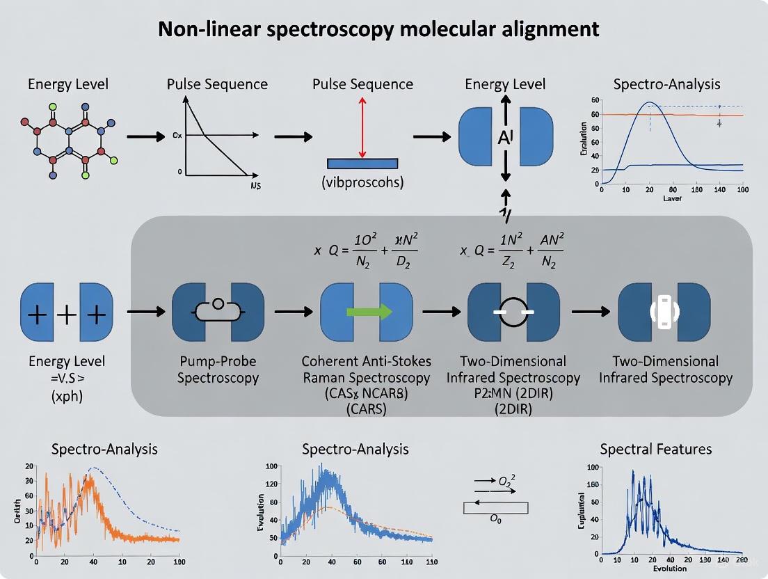
Visualization of Non-Linear Spectroscopy Concepts

Molecular Alignment Control in Non-Linear Spectroscopy

The Scientist's Toolkit: Research Reagent Solutions

Table 3: Essential Equipment and Materials for Non-Linear Spectroscopy

Item	Specifications	Function	Representative Examples
Femtosecond Laser Systems	Ti:Sapphire oscillator/amplifier, ~800 nm, 100 fs, 80 MHz rep rate [4]	Provides high peak power for multi-photon processes	FemtoFiber ultra series with fiber delivery [6]
Tunable IR Sources	OPO/OPA systems, tunable 2.5-20 μm, ps/fs pulses	Vibrational spectroscopy via SFG, CARS, SRS	TOPTICA TOPO smart for MIR region [6]
Alignment Accessories	Beam profilers, autocorrelators, delay stages	Ensures spatial/temporal overlap of multiple beams	High-precision mechanical and optical delay stages
Detection Systems	PMTs, APDs, CCD/CMOS cameras, spectrographs	Sensitive detection of weak non-linear signals	Andor EMCCD and sCMOS cameras [1]
Molecular Beam Systems	High vacuum chambers, pulsed valves, skimmers	Provides isolated molecules for alignment studies	Custom ultrahigh vacuum systems
Polarization Optics	Waveplates, polarizers, Brewster windows	Controls polarization states for selection rules	Zero-order half-wave and quarter-wave plates
Microscopy Platforms	Laser-scanning microscopes, high NA objectives	Enables 3D sectioning and cellular imaging	Nikon A1 MP+/A1R MP+ systems [4]
Sample Chambers	Environmental control, temperature, pressure	Maintains physiological conditions for living samples	Custom perfusion chambers with temperature control

Advanced Applications in Molecular Research

Non-linear spectroscopic methods have enabled groundbreaking applications in molecular research, particularly in the control and characterization of molecular alignment. Research at Sandia National Laboratories' CRF facility has demonstrated that combining adiabatic and nonadiabatic alignment approaches yields higher degrees of molecular alignment than either method alone [5]. Using femtosecond/picosecond CARS as a sensitive probe, researchers quantified alignment in molecular H₂, showing significant signal enhancement corresponding to increased molecular alignment at the spatial location where the alignment fields were focused [5]. This refined control over molecular orientation has profound implications for understanding stereochemical reaction dynamics and developing advanced molecular manipulation techniques such as optical centrifuges [5].

The unique interface specificity of techniques like SFG has been particularly valuable for characterizing biomolecular interactions at surfaces. Studies of functionalized nanoparticles and liposomes—critical systems for drug delivery and biosensing—have revealed how surface curvature affects the packing, organization, and dynamics of chemical groups at biomaterial interfaces [3]. These findings would not be predicted based on traditional two-dimensional surface models, highlighting the importance of direct measurement in biologically relevant environments. The emergence of sum-frequency scattering (SFS) and second-harmonic scattering (SHS) techniques now enables extension of these surface-specific measurements to spherical nanoparticles and other centrosymmetric structures in aqueous environments, opening new possibilities for studying biomaterials in their native biological contexts [3].

For drug development professionals, non-linear spectroscopic methods offer powerful approaches for characterizing drug-membrane interactions, protein conformation at interfaces, and the surface chemistry of drug delivery vehicles. The molecular orientation information provided by techniques like polarized SFG can reveal how therapeutic compounds orient at membrane interfaces, providing insights into mechanisms of action and supporting rational drug design [3]. Similarly, SHG imaging has been applied to characterize collagen structure and organization in tissues, providing diagnostic information about disease states and treatment effects without requiring exogenous labels [3]. As these non-linear methods continue to advance, they offer an expanding toolkit for understanding and controlling molecular interactions in complex biological systems.

Non-linear spectroscopy encompasses a suite of advanced techniques that probe light-matter interactions beyond the linear regime, typically employing high-intensity, pulsed lasers to drive multi-photon processes. These methods are pivotal in the field of molecular alignment control research, enabling scientists to precisely manipulate and probe the spatial orientation of molecules using intense laser fields [5]. The core principle involves exploiting the nonlinear polarization of a material, which depends on higher-order terms of the electric susceptibility (χ⁽ⁿ⁾ where n > 1) when subjected to strong electromagnetic fields [7]. This foundation allows techniques such as Coherent Anti-Stokes Raman Scattering (CARS), Stimulated Raman Scattering (SRS), and Second Harmonic Generation (SHG) to provide unparalleled insights into molecular structure, dynamics, and chemical composition, making them indispensable for modern chemical physics and pharmaceutical analysis [8] [5].

The ability to control molecular alignment—whether through adiabatic methods using longer laser pulses or non-adiabatic (transient) methods with ultrafast pulses—opens new avenues for studying molecular dynamics and quantum state control [5]. For instance, researchers at the Combustion Research Facility have demonstrated that combining adiabatic and nonadiabatic alignment fields can achieve a higher degree of molecular alignment in H₂ than either method alone [5]. This precise control is fundamental to advancing research in quantum computing, optical clocks, and the understanding of fundamental molecular processes [6] [5].

Fundamental Advantages and Quantitative Comparison

The transition from linear to non-linear spectroscopic methods brings forth distinct and powerful advantages, primarily centered on enhanced specificity, significant background suppression, and superior spatial and temporal resolution. The table below summarizes the key technical advantages and their operational basis.

Table 1: Key Advantages of Non-linear Spectroscopy over Linear Methods

Advantage	Technical Basis	Impact on Research
Enhanced Specificity	Exploitation of molecular vibrations (CARS, SRS) and non-centrosymmetric structures (SHG) for molecule-specific contrast [8] [7].	Enables label-free identification of chemical species, such as tracking active pharmaceutical ingredients (APIs) in solid dosages or imaging specific biomolecules [8] [9].
Background Suppression	Confinement of signal generation to a tiny focal volume (<1 femtoliter) due to the non-linear intensity dependence of multi-photon processes [7].	Virtually eliminates out-of-focus background fluorescence and scattered light, yielding high-contrast images and cleaner spectral data without confocal pinholes [7].
Superior Resolution	Inherent 3D sectioning capability and diffraction-limited spatial resolution in microscopy modalities (e.g., SRS, CARS) [7].	Allows for high-resolution 3D reconstruction of samples, resolving sub-cellular structures and material microdomains deep within tissue [7].
Deep Tissue Penetration	Use of near-infrared (NIR) excitation wavelengths, which scatter and absorb less in biological tissues compared to visible/UV light [7].	Facilitates non-invasive imaging of live biological specimens at depths exceeding 500 μm, enabling the study of intact systems [7].

These advantages are interconnected. For example, the background suppression achieved through localized excitation directly contributes to the perception of superior resolution and image contrast. Furthermore, techniques like CARS and SRS provide chemical contrast by being sensitive to specific molecular vibrations, which allows them to outperform conventional Raman spectroscopy by generating a coherent, laser-like signal that is orders of magnitude stronger [8] [7].

Experimental Protocols for Molecular Alignment and Detection

This section provides detailed methodologies for key experiments in non-linear spectroscopy, focusing on molecular alignment control and the application of coherent Raman techniques.

Protocol 1: Controlled Molecular Alignment Using Combined Laser Fields

This protocol describes a method for achieving a high degree of molecular alignment in gaseous H₂ by combining adiabatic and nonadiabatic laser pulses, as derived from research at Sandia's CRF [5].

Table 2: Reagents and Equipment for Molecular Alignment

Item	Specification/Function
Ultrafast Laser System	Femtosecond/picosecond laser source (e.g., Ti:Sapphire amplifier) for nonadiabatic alignment pulses.
Nanosecond Laser	Tunable nanosecond pulsed laser (e.g., Nd:YAG at 1064 nm) for adiabatic alignment.
Gas Cell	Chamber containing the target gas (e.g., H₂) at controlled pressure.
Beam Combiner & Optics	Mirrors, lenses, and dichroics to co-align the adiabatic and nonadiabatic laser beams.
Probe Laser for CARS	A separate ps-pulsed laser system for generating the CARS signal to probe the alignment.
Spectrometer & Detector	A spectrograph coupled to a high-sensitivity array detector (e.g., LN₂-cooled MCT array) to resolve the CARS signal [10].

Procedure:

• Sample Preparation: Introduce the molecular gas (e.g., H₂) into a purged gas cell to avoid atmospheric absorption [10].
• Nonadiabatic Alignment Pulse: Focus a short, intense femtosecond laser pulse (duration << rotational period of H₂) onto the sample. This pulse creates a coherent superposition of rotational states.
• Adiabatic Alignment Pulse: Simultaneously, focus a longer nanosecond laser pulse (duration > rotational period) co-linearly with the nonadiabatic pulse into the same sample volume. The polarization anisotropy of this field mixes excited electronic states (e.g., E,F state of H₂), enhancing the molecular polarizability and trapping molecules in pendular states [5].
• Probe the Alignment: Use a time-delayed, femtosecond/picosecond CARS (fs/ps CARS) setup to probe the degree of alignment. a. Pump & Stokes: Overlap the pump and Stokes beams (derived from the probe laser) to coherently drive a vibrational resonance in the aligned molecules. b. Probe & Signal Generation: A third, time-delayed probe beam interacts with the coherent vibration to generate the anti-Stokes CARS signal. c. Spectral Detection: Resolve the CARS signal using a spectrometer and array detector. The signal intensity at frequencies corresponding to specific rotational lines (e.g., J"=1 for H₂) is directly sensitive to the degree of molecular alignment [5].

Data Analysis: The enhancement of the CARS signal at the location of the combined aligning fields, compared to the signal with a single aligning field or no field, quantitatively indicates the higher degree of alignment achieved. The measured laser power dependence can be used to determine the polarization anisotropy of the mixed excited state [5].

Protocol 2: Noise-Suppressed Heterodyne Detection for Nonlinear Spectroscopy

This protocol outlines a general noise suppression scheme for heterodyne nonlinear spectroscopy (e.g., pump-probe, four-wave mixing), which is critical for achieving high-fidelity data and detecting weak signals [10].

Procedure:

• Experimental Setup: a. Configure a standard heterodyne detection setup where a signal field (ESig) is mixed with a strong local oscillator (LO) field (ELO) at a square-law detector. b. Introduce a second, matched photodetector (a reference detector) to measure only the intensity fluctuations of the LO beam. This can be an array detector or a single-pixel detector.
• Data Acquisition: a. Digitize the outputs from both the signal detector (Itot) and the reference detector (IRef) over the entire experimental trajectory (e.g., a 40-second scan). b. Collect data with the pump beam blocked (to characterize additive noise, ΔI_LO) and unblocked (to measure the sample signal) [10].
• Two-Step Noise Suppression Algorithm [10]: a. Step 1 - Additive Noise Suppression: Perform a linear regression between the signal detector output and a linear combination of all reference channels. This optimally utilizes the spectral correlation in the reference data to subtract the additive noise component (ΔI_LO), which is often orders of magnitude larger than the weak sample signal. b. Step 2 - Convolutional Noise Handling: The algorithm further reduces residual convolutional noise arising from the product of fluctuations in the LO and pump intensities.
• Signal Extraction: The final, processed signal yields the pure sample response (e.g., the third-order susceptibility χ⁽³⁺), free from the dominant noise sources, and can improve the signal-to-noise ratio (SNR) by 10-30 times, reaching the fundamental noise floor of the signal detector [10].

Diagram 1: Noise-suppressed heterodyne detection workflow.

Advanced Applications in Research and Development

The unique advantages of non-linear spectroscopy have led to its adoption in a wide range of cutting-edge applications, particularly in drug development and materials science.

• Pharmaceutical Analysis: Non-linear techniques are powerful tools for analyzing solid pharmaceutical materials. SHG is used to identify and monitor the crystallization of active pharmaceutical ingredients (APIs) within amorphous powder matrices, providing crucial information on polymorphism and crystallization kinetics [8]. Meanwhile, CARS and SRS microscopy enable the determination of API distribution within tablets and can even monitor drug release from dissolving carriers in real-time, offering unparalleled insight into product performance and stability [8].

• Live Bioimaging and Biomedicine: Non-linear optical microscopy has revolutionized live tissue imaging by enabling label-free, non-destructive investigation of physio-pathological processes with sub-cellular resolution [7]. Multi-modal NLO microscopy combines TPEF (to image endogenous fluorophores like NAD(P)H for metabolism), SHG (to visualize collagen fibers), and CRS (to map chemical composition via lipid and protein distributions) to provide a comprehensive functional and structural overview of vital biological specimens [7]. This is instrumental in studying cancer mechanisms, tissue engineering, and fundamental cellular functions.

• Functional Materials Characterization: Label-free vibrational spectroscopy is indispensable for the development and optimization of functional materials, such as shape-memory polymers, self-healing materials, and piezoelectric materials [9]. Techniques like SFG and 2D-IR provide insights into interfacial order, site-specific coupling, and ultrafast structural dynamics, which are critical for understanding and tailoring material properties for applications in energy, aerospace, and electronics [9].

Diagram 2: Logical flow from core techniques to advanced applications.

The Scientist's Toolkit: Essential Research Reagent Solutions

The successful implementation of non-linear spectroscopy and molecular alignment experiments relies on a suite of specialized tools and reagents. The following table details key components of this toolkit.

Table 3: Essential Research Reagent Solutions for Non-linear Spectroscopy

Category	Specific Examples	Function in Research
Laser Sources	FemtoFiber ultra FD (TOPTICA), Ultrafast Ti:Sapphire Amplifiers, Optical Parametric Amplifiers (OPAs) [6] [5] [10]	Provide high-intensity, pulsed near-IR light essential for driving non-linear processes like multi-photon absorption and harmonic generation.
Alignment & Control Systems	TeraFlash smart THz systems, CLS Sub-Hz Clock Laser Systems [6]	Enable precise temporal and spatial control of laser beams for molecular alignment experiments and ultra-stable measurements.
Detection Systems	High-sensitivity MCT array detectors, Balanced/Referenced photodetectors [10]	Capture weak non-linear signals with high signal-to-noise ratio, often in conjunction with spectrographs for spectral resolution.
Targeted Contrast Agents (Preclinical)	Antibody- or peptide-dye conjugates (e.g., EGF-Cy5.5), Quantum Dot bioconjugates [11]	Provide molecular specificity for imaging, allowing visualization of specific biomarkers (e.g., EGFR) in complex biological environments.
Non-specific Stains & Dyes	Acriflavine, Cresyl Violet, Indocyanine Green [11]	Enhance contrast for cellular and sub-cellular structures in microscopy, often used in clinical and pre-clinical screening.

Non-linear optical microscopy has emerged as a powerful toolbox for investigating molecular systems, offering exceptional resolution, deep tissue penetration, and unique chemical contrast mechanisms without the need for exogenous labeling. These techniques exploit the non-linear interactions between intense laser light and matter, providing researchers with unparalleled capabilities for studying molecular alignment, cellular metabolism, and tissue architecture. Within the context of molecular alignment control research, understanding these processes is paramount for designing experiments that can probe molecular orientation, structural organization, and dynamic processes in functional materials and biological systems. The non-linear processes covered in this application note—Second Harmonic Generation (SHG), Coherent Anti-Stokes Raman Scattering (CARS), Stimulated Raman Scattering (SRS), and Two-Photon Induced Luminescence (2P-LIF)—each provide unique advantages for specific research applications, particularly when implemented in a multimodal approach that leverages their complementary strengths [12].

The coherence and polarization sensitivity of many non-linear processes make them exceptionally well-suited for investigating molecular alignment. Unlike linear optical techniques, non-linear methods typically require high peak power lasers, most commonly ultrafast pulsed lasers with pulse widths ranging from femtoseconds to picoseconds [13] [14]. The resulting signals are confined to the focal volume, providing inherent optical sectioning capability without the need for a physical pinhole. This technical note provides a comprehensive overview of these critical non-linear processes, including their physical principles, experimental requirements, and protocols for implementation in molecular alignment control research.

Process Principles and Theoretical Foundations

Physical Mechanisms and Signal Generation

Second Harmonic Generation (SHG) is a second-order non-linear process where two photons at a fundamental frequency (ω) combine to generate a single photon at exactly twice the frequency (2ω). This process requires a non-centrosymmetric environment for signal generation, making it exquisitely sensitive to molecular order and alignment [12] [14]. SHG is a parametric process, meaning there is no energy deposition in the sample and no net energy transfer between the optical fields and the medium. The resulting signal emerges as coherent, directional radiation that preserves polarization information, making it ideal for studying molecular orientation [12].

Coherent Anti-Stokes Raman Scattering (CARS) is a third-order non-linear process that involves four-wave mixing. In CARS, a pump beam (ωp) and a Stokes beam (ωs) interact with the sample when their frequency difference (ωp - ωs) matches a molecular vibrational frequency (Ω). This interaction generates a coherent anti-Stokes signal at a higher frequency (ωas = 2ωp - ωs) [13] [14]. The CARS signal is resonantly enhanced when Ω matches molecular vibrations, providing chemical specificity. However, CARS also produces a non-resonant background that can limit contrast, particularly at low concentrations [13].

Stimulated Raman Scattering (SRS) encompasses two complementary processes: Stimulated Raman Gain (SRG) on the Stokes beam and Stimulated Raman Loss (SRL) on the pump beam. When the frequency difference between pump (ωp) and Stokes (ωs) beams matches a molecular vibrational frequency, energy is transferred between the beams, resulting in a measurable intensity gain in the Stokes beam or loss in the pump beam [15] [13]. Unlike CARS, SRS lacks a non-resonant background, provides spectra identical to spontaneous Raman, and exhibits a linear dependence on analyte concentration, enabling straightforward quantification [15] [16].

Two-Photon Induced Luminescence (2P-LIF) occurs when a molecule simultaneously absorbs two photons to reach an excited electronic state, followed by emission of a fluorescence photon. The probability of two-photon absorption depends on the square of the excitation intensity, confining the signal to the focal volume [14] [2]. This process provides high-resolution optical sectioning with reduced photobleaching in out-of-focus regions compared to single-photon fluorescence.

Table 1: Comparison of Key Non-Linear Optical Processes

Process	Non-Linear Order	Signal Type	Key Applications	Quantitative Capability
SHG	Second-order (χ²)	Coherent, forward-directed	Collagen imaging, molecular crystals	Qualitative (orientation)
CARS	Third-order (χ³)	Coherent, directional	Lipid imaging, chemical mapping	Non-linear concentration dependence
SRS	Third-order (χ³)	Intensity gain/loss	Quantitative bioimaging, metabolism	Linear concentration dependence
2P-LIF	Second-order (effectively)	Incoherent fluorescence	Cellular metabolism, deep tissue imaging	Quantitative with calibration

Energy Level Diagrams and Transition Pathways

The following energy level diagrams illustrate the fundamental transition pathways for each non-linear process:

Experimental Protocols and Methodologies

Instrumentation Setup and Configuration

Laser Source Requirements Non-linear optical processes require high peak power lasers, typically ultrafast pulsed lasers with pulse widths ranging from femtoseconds to picoseconds. For CARS and SRS, two synchronized laser sources are necessary—a pump beam and a Stokes beam—with precise temporal and spatial overlap [13] [17]. The frequency difference between these beams must be tunable to target specific molecular vibrations. Recent advances in fiber laser technology have produced compact, stable sources specifically designed for CRS microscopy, offering improved intensity stability and timing jitter as low as 24.3 fs [17].

Microscopy Configuration

• SHG Setup: Requires a high-numerical-aperture objective for tight focusing. Signal detection typically occurs in the forward direction due to the coherent, directional nature of SHG, though backward detection is possible from interfaces [14].
• CARS Configuration: Implemented with both forward (F-CARS) and backward (E-CARS) detection schemes. F-CARS provides stronger signal for larger structures, while E-CARS offers better contrast for small features due to reduced non-resonant background [14].
• SRS Setup: Typically detected in the forward direction using a high-sensitivity photodiode and lock-in amplification. The Stokes beam is modulated at high frequencies (typically MHz), and the intensity loss on the pump beam is measured [16] [17].
• 2P-LIF System: Requires a high-sensitivity detector such as a photomultiplier tube (PMT) or avalanche photodiode (APD). Detection occurs in the backward (epi) direction, similar to confocal microscopy, but without the need for a pinhole [14].

Table 2: Laser Requirements for Non-Linear Microscopy Techniques

Technique	Laser Type	Pulse Width	Synchronization Required	Key Laser Parameters
SHG	Ti:Sapphire or fiber laser	~100 fs	No	High peak power, tunable wavelength
CARS	Dual-output synchronized lasers	Ps pulses preferred	Yes	Precise timing jitter <100 fs
SRS	Dual-output synchronized lasers	Ps pulses for spectral resolution	Yes	High intensity stability, low noise
2P-LIF	Ti:Sapphire or fiber laser	~100 fs	No	High repetition rate, tunable wavelength

Sample Preparation Guidelines

Label-Free Imaging (SHG, CARS, SRS) For endogenous contrast imaging, sample preparation is minimal. Tissue sections should be cut to appropriate thickness (typically 5-20μm for ex vivo studies) and mounted on standard glass slides. For live cell imaging, cells should be cultured on coverslips designed for microscopy. The key consideration is maintaining sample integrity and molecular organization, particularly for SHG, which relies on non-centrosymmetric structure [12].

Fluorescent Probe Selection for 2P-LIF

• Endogenous Fluorophores: NAD(P)H, FAD, lipofuscin, and amyloid deposits can be imaged without exogenous labeling [12] [14].
• Synthetic Dyes: Choose fluorophores with high two-photon absorption cross-sections. Common choices include GFP variants, synthetic dyes like Rhodamine, and chemical indicators for calcium or pH.
• Quantum Dots: Offer high two-photon cross-sections and photostability but require consideration of potential toxicity in live cell experiments.

Step-by-Step Experimental Procedure

Multimodal Non-Linear Imaging Protocol This protocol describes a coordinated approach for acquiring SHG, CARS, SRS, and 2P-LIF images from the same sample region, enabling comprehensive molecular alignment analysis.

• System Alignment and Calibration

  • Turn on all laser systems and allow 30-60 minutes for thermal stabilization.
  • Align beam paths to ensure co-linear propagation of pump and Stokes beams for CARS/SRS.
  • Verify temporal overlap using a cross-correlator or second-harmonic generation crystal.
  • Calibrate wavelength tuning using a reference sample with known Raman peaks (e.g., polystyrene at 2,900 cm⁻¹ for CH stretching).

• Sample Positioning and Focus Optimization

  • Place sample on microscope stage and locate region of interest using brightfield illumination.
  • Using low laser power, optimize focus using non-linear signal as reference.
  • For polarization-sensitive measurements (particularly SHG), ensure proper alignment of polarization optics.

• Sequential Image Acquisition

  • Begin with 2P-LIF imaging using appropriate excitation wavelength for target fluorophores.
  • Acquire SHG images by tuning laser to excitation wavelength and detecting at exactly half the wavelength.
  • For CARS imaging, set pump and Stokes beams to target vibrational frequency of interest.
  • For SRS imaging, modulate Stokes beam and detect pump beam depletion using lock-in amplification.
  • Maintain consistent laser power and detector settings across comparable samples.

• Data Processing and Analysis

  • Apply background subtraction and flat-field correction to all images.
  • For quantitative SRS analysis, prepare standard solutions for concentration calibration.
  • For molecular orientation analysis from SHG, analyze polarization dependence of signal.
  • Register images from different modalities using fiduciary markers or software-based alignment.

The Scientist's Toolkit: Essential Research Reagents and Materials

Table 3: Essential Research Reagents and Materials for Non-Linear Microscopy

Item	Specifications	Application/Function
Ultrafast Laser System	Ti:Sapphire (680-1080 nm) or fiber laser (1030-1064 nm), ~100 fs pulse width	Primary excitation source for all non-linear processes
Synchronized OPO/OPA	Tunable output (e.g., 700-900 nm for OPO), ps pulses for CARS/SRS	Provides Stokes beam for coherent Raman techniques
High-NA Objective	Water or oil immersion, NA >1.2	Tight focusing for efficient non-linear excitation
Vibration Isolation Table	Active or passive isolation system	Minimizes mechanical noise for stable beam alignment
Photomultiplier Tubes	GaAsP detectors for visible range, InGaAs for NIR	High-sensitivity detection for 2P-LIF and SHG
Lock-in Amplifier	>20 MHz modulation frequency, high dynamic range	Extracts weak SRS signals from background noise
Polarization Optics	Half-wave plates, polarizing beam splitters, analyzers	Controls and analyzes polarization for molecular orientation studies
Reference Samples	Polystyrene beads, silica, urea crystals	System calibration and alignment verification
Cell Culture Materials	Coverslip-bottom dishes, appropriate media	Live cell imaging preparation

Applications in Molecular Alignment Control Research

The non-linear optical techniques described in this document provide powerful approaches for investigating molecular alignment in various research contexts:

Biological Tissue Organization SHG microscopy excels at visualizing ordered biological structures such as collagen fibrils, myosin fibers, and microtubule arrays without staining [12]. The polarization sensitivity of SHG enables quantitative analysis of fibril orientation and degree of alignment, which is crucial for understanding tissue biomechanics and pathological changes in diseases like fibrosis or cancer.

Polymer and Materials Science CARS and SRS microscopy enable chemical-specific imaging of polymer blends and composites, allowing researchers to map domain orientation and molecular order without extrinsic labeling [9]. The ability to track deuterium-labeled compounds via SRS provides exceptional capabilities for studying molecular diffusion and alignment dynamics in functional materials.

Neuroscience and Brain Imaging Multimodal non-linear imaging combining 2P-LIF, SHG, and SRS enables comprehensive investigation of brain tissue with molecular specificity [14]. Third-harmonic generation (THG) complements these techniques by providing contrast at interfaces, particularly in lipid-rich regions, offering insights into myelin organization and neuronal alignment.

Drug Development Applications In pharmaceutical research, these label-free techniques enable monitoring of drug distribution and metabolism without chemical modification that might alter bioactivity [16]. SRS imaging of small molecules containing alkyne, nitrile, or deuterium tags allows direct visualization of drug compounds in cells and tissues, providing critical information about target engagement and cellular uptake mechanisms relevant to molecular alignment with biological targets.

Advanced Technical Considerations

Spectral Focusing for Enhanced Resolution

For CARS and SRS imaging with femtosecond lasers, spectral focusing provides a method to achieve high spectral resolution while maintaining the high peak power of broadband pulses. This technique involves applying matched chirp to both pump and Stokes pulses, effectively narrowing the instantaneous bandwidth at the sample [13]. The Raman resonance can then be tuned by adjusting the relative time delay between the two pulses, enabling hyperspectral imaging without mechanical tuning of laser wavelengths.

Noise Reduction Strategies in SRS

The weak SRS signals (typically 10⁻⁴ to 10⁻⁶ of the pump beam intensity) require sophisticated noise reduction approaches. Balanced detection can suppress laser noise by 50 dB or more, but adds complexity to the experimental setup [17]. Recent advances in fiber laser technology have produced sources with intrinsic intensity noise improvements of 50 dB, enabling high-quality SRS imaging without balanced detection schemes [17].

Polarization-Sensitive Measurements

For molecular alignment studies, polarization-controlled excitation provides critical information about molecular orientation. Polarization-resolved SHG is particularly powerful for determining the orientation of non-centrosymmetric structures [12]. Similarly, polarization-sensitive CARS and SRS can reveal molecular orientation by analyzing the dependence of Raman signals on the polarization direction relative to molecular axes.

The continued development of these non-linear optical techniques, particularly in compact, robust laser sources and improved detection schemes, promises to expand their applications in molecular alignment control research across biology, materials science, and drug development.

Molecular alignment control is a cornerstone of advanced materials science and drug development, enabling the precise manipulation of molecular orientation to dictate fundamental material properties. The anisotropic arrangement of molecules directly governs critical behaviors including nonlinear optical (NLO) activity, mechanical strength, and catalytic efficiency [18] [19]. Probing and quantifying this directional dependence provides transformative insights into structural organization at the molecular level, offering significant scientific and industrial benefits [18]. Nonlinear vibrational spectroscopy has emerged as a powerful toolset for both analyzing and actively controlling molecular alignment, bridging the gap between fundamental theoretical principles and practical application across diverse systems—from polymer composites and organic crystals to complex biomedical tissues [18] [9]. These label-free techniques deliver real-time, high-resolution, and non-destructive insights into molecular and functional properties, thereby accelerating innovation in material design [9]. This document outlines the theoretical foundations, measurement methodologies, and detailed experimental protocols for molecular alignment control, providing researchers with a comprehensive framework for implementation.

Theoretical Foundations and Key Relationships

The theoretical framework for molecular alignment control is rooted in the interaction of light with anisotropic molecular systems. The following principles are fundamental.

Theoretical Basis of Alignment-Property Relationships

Molecular alignment refers to the non-random, directional orientation of molecules within a material system. This orientation is not merely structural but fundamentally dictates macroscopic observable properties. The control over alignment allows for the fine-tuning of material responses.

• Nonlinear Optical (NLO) Activity: In host-guest systems, the electro-optic (EO) activity, such as the Pockels effect, arises from the noncentrosymmetric alignment of dipolar chromophores within a polymer matrix after electric field poling. The key performance metric, the electro-optic tensor element ( r_{33} ), depends directly on the molecular hyperpolarizability ( \beta ) and the order parameter ( \langle \cos^3 \theta \rangle ), where ( \theta ) is the angle between the molecular dipole moment and the poling field direction [19].
• Spectroscopic Activity: For a molecule with N atoms, its 3N-6 vibrational normal modes are probed by techniques like FTIR and Raman spectroscopy. The activity and intensity of these modes are highly sensitive to molecular orientation relative to the polarization of incident light. A vibration is IR-active if it results in a change in the molecular dipole moment, while Raman scattering involves a change in polarizability [9].
• Stability and Aggregation: At high number densities or elevated temperatures, strongly dipolar or zwitterionic chromophores tend to aggregate. The type and size of aggregates significantly alter the NLO response, which can be attenuated, amplified, or otherwise modified based on the mutual molecular arrangement within the aggregate [19].

Quantitative Descriptors of Molecular Alignment

Quantifying alignment is essential for correlating structure with function. The table below summarizes key descriptors derived from computational and experimental analyses.

Table 1: Key Quantitative Descriptors for Molecular Alignment Analysis

Descriptor Name	Definition/Calculation	Information Conveyed	Applicable System
Order Parameter (( \langle \cos^3 \theta \rangle ))	Average of ( \cos^3 \theta ) over an ensemble of molecules, where ( \theta ) is the angle between a molecular axis (e.g., dipole) and a reference director (e.g., electric field).	Degree of polar order and poling efficiency; directly relates to EO coefficient ( r_{33} ) [19].	Electric-field-poled chromophore/polymer systems.
Degree of Molecular Alignment (DMA) [20]	A quantified value based on distances and angles between lower axial CH bonds and surface metal atoms.	Stability of adsorption configurations; linearly related to adsorption energy for saturated cyclic compounds on metal surfaces [20].	Molecules adsorbed on catalytic surfaces (e.g., Pd(111), Pt(111)).
Aggregate Size Distribution [19]	Frequency distribution of the number of chromophore molecules involved in a single aggregate.	Reveals phase separation behavior and helps identify loading thresholds beyond which EO performance degrades.	High-density chromophore guest-host materials.
Vector Maps [18]	In-plane orientation vectors derived from polarized FTIR data, calculated for each vibrational mode.	Reveals in-plane molecular orientation and anisotropy in heterogeneous systems like polymers and human osteons.	FTIR-imaged samples (fibers, tissues, crystals).

Measurement Methodologies and Workflows

Advanced spectroscopic and computational methods form the backbone of molecular alignment analysis. The following workflow illustrates the integrated process from sample preparation to data analysis.

Spectroscopic Techniques for Alignment Analysis

• Linear Vibrational Spectroscopy: Conventional Fourier-Transform Infrared (FTIR) spectroscopy, especially when coupled with polarization control, is a workhorse for measuring molecular orientation. The spatial resolution of far-field IR microscopy is, however, diffraction-limited to a few micrometers [9]. Attenuated Total Reflection (ATR)-FTIR is particularly advantageous for analyzing thin films and surfaces with minimal sample preparation [9].
• Nonlinear Vibrational Spectroscopy: Techniques like Sum-Frequency Generation (SFG) are inherently surface-sensitive, isolating non-centrosymmetric interfaces (e.g., solid/liquid) and providing exceptional insights into interfacial molecular order [9]. Coherent anti-Stokes Raman Scattering (CARS) and Stimulated Raman Scattering (SRS) enable label-free chemical imaging with high spatial and temporal resolution, ideal for investigating dynamic processes within functional materials [9].
• Nano-Scale IR Spectroscopy: To overcome the diffraction limit, techniques like AFM-IR and Photoinduced Force Microscopy (PiFM) have been developed. These methods use an AFM tip as a nanoscale optical antenna, mapping IR-induced thermal expansion or force interactions with spatial resolutions down to ~20 nm, allowing for the chemical mapping of fine material microdomains [9].

Computational and Analysis Tools

• The "4+ Angle Polarization" Widget: This innovative toolbox within the open-source Quasar platform (https://quasar.codes/) streamlines the advanced analysis of complex microspectroscopic datasets. It enables precise in-plane molecular orientation analysis from multiple-angle polarized FTIR (p-FTIR) data, overcoming the limitations of traditional two-angle methods and generating representative vector maps for each vibrational mode [18].
• Python-Based Aggregation Analysis Tool: A novel computational tool has been developed for the detailed analysis of aggregation and phase behavior from Molecular Dynamics (MD) simulation trajectories. This tool provides frequency distributions of aggregate size and type, offering direct, countable insights into chromophore organization at the atomistic level, which is difficult to ascertain experimentally [19].
• Molecular Representation Learning: Modern AI-driven methods, particularly 3D-aware graph neural networks (GNNs), are catalyzing a paradigm shift. These models learn continuous molecular embeddings that capture spatial geometry and electronic features critical for modeling molecular interactions and conformational behavior, thereby enhancing property prediction and material design [21].

Detailed Experimental Protocols

Protocol: In-Plane Molecular Orientation Analysis Using p-FTIR and Quasar

This protocol details the procedure for determining in-plane molecular orientation in a fibrous sample using polarized FTIR and the Quasar software platform [18].

• Research Reagent Solutions:

  • Sample Material: Polylactic acid (PLA) organic crystals, murine cortical bone, or human osteons.
  • Software: Open-source Quasar platform installed from https://quasar.codes/.
  • Instrumentation: FTIR spectrometer coupled with an infrared microscope equipped with a programmable motorized stage and a linear polarizer.

• Procedure:

  • Sample Sectioning: For solid samples like bone or polymer fibers, prepare thin sections (e.g., 5-10 µm thick) using a microtome and mount on IR-transparent windows.
  • Data Acquisition: a. Locate the region of interest using the microscope. b. Using the "4+ Angle Polarization" widget in Quasar, define the acquisition parameters, including the number of polarization angles (≥4) and the spectral range. c. The widget will automatically rotate the polarizer and acquire a spectral stack at each defined angle.
  • Data Processing: a. The widget internally performs atmospheric correction and baseline subtraction. b. For each vibrational mode of interest, the software fits the recorded absorbance as a function of the polarization angle to a sinusoidal function.
  • Orientation Vector Mapping: a. The widget calculates the in-plane orientation angle and degree of anisotropy for each pixel and each vibrational mode. b. The output is a vector map overlaid on the chemical image, visually representing the in-plane molecular orientation.
  • Interpretation: Analyze the vector maps to identify domains of uniform alignment, defects, and correlations between the orientation of different functional groups.

Protocol: Analyzing Chromophore Aggregation via Molecular Dynamics

This protocol describes how to use MD simulations and the novel Python-based analysis tool to investigate aggregation behavior in chromophore-polymer composite systems [19].

• Research Reagent Solutions:

  • Software: BIOVIA Materials Studio (for MD simulation with COMPASS III force field), custom Python analysis script.
  • Model Components: Atactic poly(methyl methacrylate) (PMMA) host polymer chains and a variable number of dipolar chromophore (e.g., C3) guest molecules.

• Procedure:

  • Model Construction: a. Build a simulation cell containing 3 PMMA chains (100 repeat units each) and a variable number of chromophore molecules (e.g., 7-28 molecules for 10-30 wt%) using a Monte Carlo packing algorithm. b. Perform an annealing stage at the poling temperature (e.g., 450 K) to equilibrate the model.
  • Electric Field Poling Simulation: a. Stage 1: Apply an electric field at a temperature above the glass transition temperature (T₉) to facilitate chromophore alignment. b. Stage 2: Continue applying the field while cooling the system to room temperature (300 K) to "freeze in" the alignment. c. Stage 3: Remove the electric field and simulate at a slightly elevated temperature to study relaxation and alignment stability.
  • Trajectory Analysis: a. Extract the coordinates of chromophores from the MD trajectory files for the stages of interest. b. Run the Python analysis script to identify aggregates. The script typically uses distance and angle criteria between key atoms on different chromophores to define an aggregate.
  • Generate Distribution Data: a. The script outputs frequency distributions of aggregate sizes (number of chromophores per aggregate) and types (e.g., parallel, anti-parallel, H-aggregate, J-aggregate). b. Visualize the aggregates within the simulation cell to understand their spatial distribution and morphology.
  • Correlate with Properties: Calculate the order parameter ( \langle \cos^3 \theta \rangle ) from the same trajectory and correlate its temporal evolution with the growth of specific aggregate types and sizes.

The Scientist's Toolkit

Table 2: Essential Research Reagents and Tools for Molecular Alignment Studies

Item Name	Function/Application	Key Features / Rationale for Use
Quasar Software Platform [18]	Open-source platform for advanced spectroscopic data analysis, specifically p-FTIR.	Contains the "4+ Angle Polarization" widget for streamlined, accurate orientation analysis beyond traditional methods.
Polarized FTIR Microscope [18] [9]	Measurement of orientation-dependent IR absorption for anisotropic samples.	Combines chemical specificity with spatial resolution; enables molecular-level insights into structural orientation.
Python Aggregation Analysis Tool [19]	Analysis of MD trajectories to quantify chromophore aggregation.	Provides direct, atomistic-level insights into aggregate size/type distributions, complementing experimental data.
COMPASS III Force Field [19]	MD simulations of organic and inorganic materials, including host-guest systems.	Validated for polymers and chromophores; enables accurate modeling of non-bonded interactions critical for aggregation.
Nonlinear Spectrometer (SFG/SRS) [9]	Probing interfacial molecular order (SFG) and high-resolution chemical imaging (SRS).	Provides surface-specificity (SFG) and breaks diffraction limit for vibrational imaging, revealing sub-micron alignment.
Dipolar Chromophore (e.g., C3) [19]	Active NLO component in guest-host electro-optic materials.	High hyperpolarizability (β) and dipole moment; serves as a model system for studying poling and aggregation.

Interpreting data from molecular alignment studies requires a multi-modal approach. Correlate vector maps from p-FTIR with aggregate analysis from MD simulations to build a comprehensive model of the system's structure-property relationships. For instance, a decline in the EO coefficient ( r_{33} ) can be due to a loss of overall order (decreasing ( \langle \cos^3 \theta \rangle )) or the formation of centrosymmetric aggregates that cancel out the NLO response, even if local order is high. The power of nonlinear spectroscopy lies in its ability to disentangle such complex scenarios, providing unambiguous, label-free fingerprints of molecular organization and dynamics at multiple length scales.

The methodologies outlined herein—from the practical Quasar widget to the predictive power of AI-driven representations and MD analysis—provide a robust foundation for advancing the field of molecular alignment control. Their application accelerates the targeted design of functional materials for photonics, biomedical devices, and sustainable technologies.

Nonlinear spectroscopy provides a powerful suite of techniques for probing and controlling molecular alignment and structure with exceptional resolution and specificity. These methods rely on the interaction of matter with multiple photons from high-intensity laser sources [22]. The precise configuration of these laser systems and their associated instrumentation is paramount for successful experimentation, particularly in advanced applications such as controlling molecular alignment for structural biology and drug development [23] [3]. This document outlines the essential laser requirements, system configurations, and experimental protocols for nonlinear spectroscopy within the context of molecular alignment control research.

Laser System Requirements

The core of a nonlinear spectroscopy setup is a high-intensity laser system, typically offering ultrafast pulses. The specific parameters—such as pulse duration, wavelength, intensity, and repetition rate—must be carefully selected to match the intended nonlinear process and the molecular system under investigation [1] [24].

Table 1: Essential Laser Parameters for Common Nonlinear Spectroscopies

Laser Parameter	Typical Range	SHG/ SFG	CARS/ SRS	Molecular Alignment	Rationale & Impact
Pulse Duration	Femtoseconds (fs) to Picoseconds (ps)	●	●	●	Ultrafast pulses provide high peak power for efficient nonlinear excitation while minimizing sample damage [1].
Pulse Energy	µJ to mJ	●	●	●	Directly influences the strength of the nonlinear signal; higher orders require more intense fields [1].
Wavelength	UV to Near-IR (Tunable)	●	●	●	Must match electronic/vibrational resonances for enhancement; tunability is key for spectroscopy [25] [3].
Repetition Rate	kHz to MHz	●	●	●	Balances signal averaging speed with pulse energy and thermal load on the sample [1].
Peak Intensity	10¹² – 10¹⁴ W/cm²	◐	◐	●	Critical for strong-field processes like laser-induced molecular alignment [24].
Polarization Control	Linear, Circular, Elliptical	●	●	●	Essential for probing molecular symmetry and for multidimensional alignment control [23] [24].

Legend: ● Critical Parameter, ◐ Situation-Dependent Importance

Experimental Protocols

Protocol for Laser-Induced Molecular Alignment

Laser-induced alignment utilizes the interaction between a molecule's anisotropic polarizability and the electric field of a laser pulse to fix molecules in space, a breakthrough technique that significantly improves structural resolution in imaging techniques like single-particle diffractive imaging (SPI) [23] [26].

Objective: To achieve geometric confinement (alignment) of macromolecules in a gas-phase or molecular beam for enhanced structural analysis. Primary Applications: Pre-aligning proteins and nanoparticles for X-ray free-electron laser (XFEL) imaging; fundamental studies of strong-field molecular dynamics [23] [24].

Materials & Reagents:

• Pulsed, high-intensity laser system (e.g., Ti:Sapphire amplifier)
• Molecular beam source (e.g., supersonic jet)
• Polarization optics (wave plates, polarizers)
• Vacuum chamber
• Detection system (e.g., mass spectrometer, ion imaging detector, XFEL)

Procedure:

• Sample Preparation: Introduce the sample (e.g., protein solution) into a vacuum chamber via a supersonic jet expansion to form a cold, gas-phase molecular beam [23].
• Laser Configuration:
  • Utilize a linearly or elliptically polarized laser pulse in the intensity range of 10¹² – 10¹⁴ W/cm² [24].
  • Pulse duration should be on the order of the molecular rotational period (typically femtoseconds to picoseconds) [24].
• Alignment Mechanism:
  • The laser pulse induces a transient electric dipole moment in the molecules.
  • The interaction potential ( U = -\mu_{\text{ind}} \cdot E ) causes a torque, forcing the molecules to rotate until their most polarizable axis is parallel to the laser's polarization vector [23] [26] [24].
• Alignment Type:
  • Adiabatic Alignment: Achieved with a slowly varying laser pulse (duration >> rotational period). The molecules remain aligned only during the pulse [24].
  • Nonadiabatic (Field-Free) Alignment: Achieved with an ultrashort pulse (duration << rotational period). The laser pulse creates a coherent rotational wave packet that leads to periodic revivals of alignment after the pulse has ended [24].
• Validation & Analysis:
  • The degree of alignment is quantified by the ensemble-averaged alignment parameter, ( \langle \cos²\theta \rangle ), where ( \theta ) is the angle between the molecular axis and the laser polarization. An isotropic distribution yields 1/3, while perfect alignment yields 1 [24].
  • Alignment is typically verified using techniques like Coulomb explosion imaging or by analyzing the improved resolution in subsequent X-ray diffraction patterns [23] [24].

Protocol for High-Resolution Nonlinear Mixing Spectroscopy

This protocol is for techniques like Four-Wave Mixing (FWM), which can achieve high spectral resolution and eliminate inhomogeneous broadening without requiring the sample to fluoresce [25].

Objective: To obtain high-resolution, site-selective spectra from specific components within a complex mixture or inhomogeneously broadened sample. Primary Applications: Ultra-trace analysis of inorganic and organic materials; studying specific sites in doped crystals [25].

Materials & Reagents:

• Two or more tunable, narrow-bandwidth pulsed lasers.
• Sample environment (e.g., cryostat for low-temperature studies).
• Precision optics for beam collimation, focusing, and recombination.
• Photodetector or spectrometer for signal acquisition.

Procedure:

• System Configuration:
  • Two or more tunable laser beams are spatially and temporally overlapped within the sample.
  • The beams are arranged in a phase-matching geometry (e.g., BoxCARS) to ensure the nonlinear signal is emitted in a separable direction [25] [1].
• Selective Excitation:
  • Tune the frequencies of the incident lasers to be resonant with electronic, vibrational, or vibronic transitions of a specific target molecule or a specific site within an inhomogeneous distribution [25].
• Signal Generation:
  • The nonlinear interaction, described by the third-order susceptibility ( \chi^{(3)} ), generates a new coherent beam at a frequency that is a combination of the input frequencies (e.g., ( \omega{\text{sig}} = \omega1 + \omega2 - \omega3 ) ) [25] [1].
  • This signal is resonantly enhanced when the laser frequencies match transitions in the sample, providing high selectivity.
• Data Collection:
  • The signal is isolated from the input beams using a combination of spatial filtering (via phase-matching) and spectral filtering (using a monochromator or spectrograph) [1].
  • The signal intensity is measured as a function of the tunable laser wavelengths to construct a spectrum.
• Analysis:
  • The resulting spectrum is dominated by contributions from the resonantly excited species, effectively isolating them from other components and eliminating inhomogeneous broadening [25].

System Workflow and Signal Detection

The following diagram illustrates a generalized workflow for a nonlinear spectroscopy experiment, from laser preparation to signal detection and analysis.

Generalized Nonlinear Spectroscopy Workflow

The Scientist's Toolkit: Essential Research Reagents and Materials

Table 2: Key Reagents and Materials for Nonlinear Spectroscopy and Alignment

Item	Function & Application
Ultrafast Amplifier	Generates high-energy, short-duration laser pulses necessary to drive nonlinear optical processes [1].
Optical Parametric Amplifier (OPA)	Down-converts the primary laser output to provide widely tunable wavelengths required for resonant excitation of specific molecular transitions [3].
Polarization Optics	Controls the polarization state (linear, circular, elliptical) of the laser beams, which is critical for molecular alignment and for probing molecular symmetry [24].
Cryostat	Cools samples to cryogenic temperatures (e.g., 2 K), which reduces thermal broadening, enhances spectral resolution, and can improve the degree of laser-induced alignment [25] [23].
Supersonic Jet Source	Creates a cold, collision-free molecular beam for gas-phase studies, essential for high-resolution spectroscopy and for effective laser-induced alignment of molecules [23].
Beam Profiling Camera	Characterizes the spatial intensity profile and position of laser beams, ensuring optimal focus and overlap at the sample position [1].
Scientific Camera (sCMOS/CCD)	Used for frequency-domain detection of nonlinear signals when coupled to a spectrograph, offering high sensitivity and multi-channel advantage [1].
Nonlinear Optical Crystals	Used for frequency conversion (e.g., SHG, SFG) and for characterizing laser pulse properties (e.g., autocorrelation).

Practical Implementation: Non-Linear Spectroscopy Techniques for Molecular Analysis

Second Harmonic Generation (SHG) for Crystal Identification and Phase Boundary Analysis

Second Harmonic Generation (SHG) is a powerful second-order nonlinear optical process where two photons of frequency ( \omega ) combine in a non-centrosymmetric medium to generate a single photon at double the frequency ( 2\omega ) [27] [28]. This Application Note details the use of SHG microscopy as a robust, label-free tool for crystal identification and phase boundary analysis, with a specific focus on its application in molecular alignment control research. We provide foundational principles, structured experimental protocols, and a detailed toolkit to enable researchers to leverage SHG for characterizing crystalline structures, polymorphs, and domain boundaries with high specificity and spatial resolution.

Second Harmonic Generation is a coherent nonlinear optical process that arises from the nonlinear polarization of a medium under intense illumination, typically from a pulsed laser [27]. The induced second-order nonlinear polarization ( P_{2\omega} ) is described by ( P(2\omega) = \chi^{(2)} E(\omega) E(\omega) ), where ( \chi^{(2)} ) is the second-order nonlinear susceptibility tensor of the material and ( E(\omega) ) is the incident electric field [28]. A fundamental prerequisite for a non-zero ( \chi^{(2)} ) and, consequently, for the observation of a dipolar SHG signal, is that the material must be non-centrosymmetric [27] [28]. In materials with inversion symmetry, the ( \chi^{(2)} ) tensor vanishes under the electric dipole approximation, prohibiting SHG. This inherent property makes SHG exquisitely sensitive to structural symmetry, forming the basis for its use in crystal identification and the analysis of polar domains and phase boundaries [29] [28]. Unlike fluorescence, SHG is a coherent and instantaneous process, free from photobleaching, and provides an endogenous contrast mechanism without the need for staining [27].

Applications in Crystal and Phase Analysis

The application of SHG in materials science and solid-state chemistry leverages its direct sensitivity to crystallographic symmetry and polar order.

• Crystal Identification and Polymorph Screening: Different crystalline polymorphs of an Active Pharmaceutical Ingredient (API) often possess distinct symmetry properties. A centrosymmetric polymorph will produce no SHG signal, while a non-centrosymmetric one will. SHG microscopy can rapidly screen powder samples or crystalline slurries, identifying and mapping the spatial distribution of polymorphs based on their intrinsic nonlinear optical response [28].
• Phase Boundary Analysis and Domain Imaging: In ferroelectric, ferroelectric nematic, or other polar materials, the SHG signal is highly sensitive to the direction of the polar axis [29]. SHG microscopy can visualize anti-parallel domains and map phase boundaries in situ with sub-micrometer resolution. This is crucial for understanding domain wall dynamics and the effects of external stimuli (electric field, temperature, stress) on material microstructure [29] [30].
• Defect Engineering: Crystal defects can locally break inversion symmetry, enabling SHG even in otherwise centrosymmetric materials. Controlled defect engineering has been demonstrated to dramatically enhance the SHG intensity of certain materials, such as KBe(2)BO(3)F(_2) (KBBF), by nearly an order of magnitude [30]. SHG serves as a direct probe for monitoring these symmetry-breaking defects.

Quantitative Data and Material Performance

The efficiency of SHG materials is quantified by their second-order susceptibility ( \chi^{(2)} ) and their performance relative to standard materials like Beta-Barium Borate (BBO).

Table 1: Performance of Selected SHG Crystals for Long-Wavelength IR Pumping

Crystal	Chemical Formula/Description	Key SHG Performance (IR Pump 1200-2000 nm)	Notable Properties
DAST	trans-4-[4-(dimethylamino)-N-methylstilbazolium] p-tosylate	Outperforms BBO [31]	Efficient organic THz generator, high ( \chi^{(2)} ) [31]
DSTMS	4-N,N-dimethylamino-4'-N'-methylstilbazolium 2,4,6-trimethylbenzenesulfonate	Outperforms BBO [31]	Efficient organic THz generator, high ( \chi^{(2)} ) [31]
PNPA	(E)-4-((4-nitrobenzylidene)amino)-N-phenylaniline	Outperforms BBO [31]	Recently discovered organic generator [31]
BBO	Beta-Barium Borate	Reference material	Common inorganic crystal, less effective at longer IR wavelengths [31]

Table 2: SHG Enhancement Strategies in Low-Dimensional and Thin-Film Materials

Strategy	Mechanism	Exemplified Material/Platform	Achieved Enhancement/Performance
Field Enhancement Heterostructures	Boosts electric field amplitude and gradient at the nonlinear material [32]	h-BN on Au/SiO2 heterostructure	SHG enhanced by two orders of magnitude [32]
Photogalvanic Effect	Optically induced space-charge gratings create effective ( \chi^{(2)} ) and enable quasi-phase-matching [33]	Si(3)N(4) microresonator	On-chip green power up to 5.3 mW, 141%/W conversion efficiency [33]
Defect Engineering	Intrinsic breaking of centrosymmetry via controlled growth conditions [30]	KBBF crystal	SHG enhanced by nearly one order of magnitude [30]
Resonant Excitation	Two-photon excitation energy resonates with exciton energy [28]	2D Materials (e.g., MoS(_2))	SHG efficiency increased up to three orders of magnitude [28]

Experimental Protocols

Protocol: SHG Microscopy for Crystal Polymorph Identification

Objective: To identify and spatially resolve different polymorphic forms in a crystalline sample of an API based on their SHG activity.

• Sample Preparation:

  • Prepare a thin film of the crystalline material on a glass slide or disperse the powder in an inert, non-birefringent medium (e.g., certain polymers or oils) between a microscope slide and coverslip to minimize scattering.

• Instrument Setup:

  • Laser Source: Utilize a mode-locked Ti:Sapphire laser tuned to the NIR-I region (e.g., 700-1000 nm) for optimal penetration and minimal linear absorption [27]. Typical pulse duration: ~100 fs; repetition rate: ~80 MHz.
  • Microscope: An inverted or upright laser-scanning microscope equipped with a high numerical aperture (NA > 1.0) objective is required to tightly focus the excitation beam and efficiently collect the emitted signals [27].
  • Detection: Collect the backward-scattered (epi) SHG signal. For thin samples, forward-scattered SHG can also be collected with a high-NA condenser [27]. Use a high-quality short-pass dichroic mirror to separate the excitation light from the SHG signal. A bandpass filter centered at half the excitation wavelength (e.g., 400-500 nm for an 800 nm pump) is placed before the detector to isolate the SHG signal from any residual fluorescence or scattered laser light. A photomultiplier tube (PMT) or a high-sensitivity CCD is used for detection.

• Data Acquisition and Analysis:

  • Acquire images at low laser power first to avoid optical damage.
  • Crystalline domains exhibiting bright SHG signal are identified as non-centrosymmetric polymorphs.
  • Areas with no SHG signal are either centrosymmetric polymorphs or amorphous material.
  • The SHG intensity can be quantified and used to create a spatial map of polymorph distribution.

Protocol: Mapping Phase Boundaries in Ferroelectric Nematic Fluids

Objective: To visualize polar domains and map phase boundaries in a ferroelectric nematic fluid via polarization-resolved SHG.

• Sample Preparation:

  • Fabricate cells with photoalignment layers to create tailored polar orientational patterns, confining the ferroelectric nematic fluid (e.g., RM734) [29]. Control cell thickness precisely using spacers.

• Instrument Setup:

  • Follow the setup in Protocol 4.1, with the critical addition of polarization optics.
  • Place a linear polarizer and a half-wave plate in the excitation path to control the polarization of the incident laser beam.
  • Place an analyzer (another linear polarizer) in the detection path before the SHG filter and PMT.

• Data Acquisition and Analysis:

  • Rotate the polarization of the incident beam while keeping the analyzer fixed, or vice versa.
  • Acquire SHG images at different polarization combinations.
  • The SHG intensity from a domain will be maximized when the incident polarization is aligned with the principal molecular axis and the analyzer is parallel to the induced nonlinear polarization.
  • Domains with opposite polarity will exhibit maximum SHG signal at orthogonal input polarizations. The boundaries between these bright and dark domains are the phase boundaries [29].

The Scientist's Toolkit: Key Research Reagents and Materials

Table 3: Essential Materials for SHG Experiments in Crystal Analysis

Item	Function/Benefit	Example Use-Cases
Organic Ionic Crystals (DAST, DSTMS)	High second-order susceptibility ( \chi^{(2)} ); effective for long-wavelength IR pumping [31]	High-efficiency frequency conversion, THz generation [31]
Ferroelectric Nematic Fluids (e.g., RM734)	Exhibit giant and switchable polar order, enabling reconfigurable SHG-active patterns [29]	Study of polar domain dynamics, prototype photonic devices [29]
Ultra-low loss Si(3)N(4) waveguides	CMOS-compatible platform; photogalvanic effect induces effective ( \chi^{(2)} ) for on-chip SHG [33]	On-chip tunable visible light sources, integrated quantum optics [33]
2D Noncentrosymmetric Materials (e.g., 3R-MoS(2), NbOCl(2))	Atomic-scale thickness, strong light-matter interaction, large ( \chi^{(2)} ) [32] [28]	Nanoscale nonlinear light sources, valleytronics, quantum light generation [32] [28]
High-Q Microresonators	Confines light to enhance intensity, boosting nonlinear efficiency via resonant enhancement [33]	Efficient frequency conversion with low pump power, frequency comb generation [33]

Workflow and Signaling Pathway Visualization

Coherent Anti-Stokes Raman Scattering (CARS) for Chemical Contrast and Drug Distribution Mapping

Coherent Anti-Stokes Raman Scattering (CARS) microscopy represents a powerful nonlinear vibrational spectroscopy technique that has established itself as an indispensable tool for investigating molecular systems with high chemical specificity. As a nonlinear variant of Raman spectroscopy, CARS combines powerful Raman signal enhancement with label-free detection capabilities, making it particularly valuable for biological and materials research. Unlike conventional Raman scattering, CARS is a four-wave mixing process that generates a coherent signal at the anti-Stokes frequency, providing several orders of magnitude stronger signals compared to spontaneous Raman scattering. This signal enhancement enables rapid imaging of biological samples and materials without the need for fluorescent labels or exogenous contrast agents, thereby preserving the native state of the system under investigation.

The fundamental principle underlying CARS involves the coherent excitation of molecular vibrations when the frequency difference between a pump beam (ω₁) and a Stokes beam (ω₂) matches the frequency of a specific molecular vibration (Ω). This vibrational resonance results in the generation of a strong anti-Stokes signal at frequency ωCARS = 2ω₁ - ω₂. The CARS signal intensity is proportional to the square of the third-order nonlinear susceptibility (|χ⁽³⁾|²) and depends on the product of the pump and Stokes beam intensities (I₁²I₂). This nonlinear dependence provides inherent three-dimensional resolution without the need for a pinhole, similar to other multiphoton microscopy techniques. The CARS process fundamentally detects Raman-active vibrational modes, offering chemical contrast based on the intrinsic molecular vibrations of the sample.

Table 1: Comparison of Vibrational Spectroscopy Techniques

Technique	Process Order	Signal Mechanism	Key Advantages	Primary Limitations
CARS	Third-order (χ⁽³⁾)	Coherent anti-Stokes scattering	High speed, inherent 3D resolution, reduced photodamage	Non-resonant background, spectral distortion
Spontaneous Raman	Linear	Inelastic scattering	Direct spectral interpretation, no non-resonant background	Slow acquisition, weak signals
SRS	Third-order (χ⁽³⁾)	Stimulated Raman gain/loss	Background-free, linear concentration dependence	Technical complexity, requires high stability
IR Absorption	Linear	Direct absorption	Simple implementation, strong signals for polar bonds	Water interference, poor spatial resolution

Fundamental Principles and Theoretical Framework

Molecular Basis of CARS Spectroscopy

The CARS process relies on the third-order nonlinear polarization P⁽³⁾ induced in a medium by the interaction of three input fields. Quantum mechanically, CARS involves a four-wave mixing process where three photons (pump, Stokes, and probe) interact with the molecular system to generate a fourth photon at the anti-Stokes frequency. The energy level diagram for CARS shows that when the difference between pump (ω₁) and Stokes (ω₂) frequencies matches a molecular vibrational frequency (Ω), vibrational coherence is established in the system. A subsequent probe photon (typically at the pump frequency) is then scattered from this coherent vibration to generate the anti-Stokes signal at ωCARS = 2ω₁ - ω₂.

The CARS signal intensity can be expressed as: ICARS ∝ |χ⁽³⁾|² I₁² I₂ where χ⁽³⁾ is the third-order nonlinear susceptibility, and I₁ and I₂ are the intensities of the pump and Stokes beams, respectively. The nonlinear susceptibility contains both resonant (χR) and non-resonant (χNR) components: χ⁽³⁾ = χR + χNR The resonant component χR provides the vibrational contrast and displays a dispersive line shape due to the interference between resonant and non-resonant contributions, which can complicate spectral interpretation but also provides enhanced sensitivity for certain applications.

CARS Process Overview

Advanced Coherent Raman Phenomena

Recent developments in coherent Raman spectroscopy have expanded beyond conventional CARS microscopy. The first experimental observation of Coherent Anti-Stokes Hyper-Raman Scattering (CAHRS) has been reported, representing a fifth-order nonlinear process that combines hyper-Raman scattering with coherent Raman scattering [34]. CAHRS relies on a six-wave mixing process described by the fifth-order nonlinear susceptibility χ⁽⁵⁾ and generates signals at ωCAHRS = 4ω₁ - ω₂. This advanced technique offers access to hyper-Raman active vibrations with different selection rules compared to conventional Raman, potentially enabling detection of "silent modes" that are inactive in both IR and Raman spectroscopy [34]. The CAHRS signal polarization is given by: PCAHRS,i⁽⁵⁾ = χijklmn⁽⁵⁾(4ω₁-ω₂; ω₁, ω₁, ω₁, ω₁, -ω₂) Ej(ω₁) Ek(ω₁) El(ω₁) Em(ω₁) E_n*(ω₂)

The phase-matching condition for CAHRS is more stringent than for CARS, requiring k_CAHRS = 4k₁ - k₂, which typically necessitates non-collinear beam geometries or high numerical aperture objectives to satisfy. The development of such advanced coherent Raman techniques significantly expands the toolbox available for molecular alignment control research, providing additional avenues for investigating molecular systems with complementary selection rules and sensitivity [34].

CARS Instrumentation and Experimental Setup

Core System Components

A typical CARS microscopy system requires several key components for efficient signal generation and detection. The primary light sources are ultrafast lasers producing pulses with durations typically in the picosecond or femtosecond range. The most common configuration involves a fixed-wavelength picosecond laser (often at 1064 nm or 1030 nm) serving as the Stokes beam, and a tunable laser system (such as an optical parametric oscillator or optical parametric amplifier) as the pump/probe beam. The tunable source must provide wavelength coverage across the vibrational frequencies of interest, typically from 500 cm⁻¹ to 3500 cm⁻¹. For multiplex CARS, where entire spectral regions are acquired simultaneously, a broadband laser source is employed for the pump beam, while a narrowband source serves as the Stokes beam.

The optical setup must ensure precise spatial and temporal overlap of the pump and Stokes beams. This is achieved using a combination of dichroic mirrors, delay stages, and autocorrelators. The beams are directed into a laser-scanning microscope equipped with high numerical aperture objectives (typically NA > 1.0) to achieve tight focusing and maximize signal generation. The forward-propagating CARS signal is collected using a condenser lens, while the epi-directed (backscattered) signal can be collected through the same objective in heterogeneous samples. Detection is typically accomplished using photomultiplier tubes, avalanche photodiodes, or CCD cameras for multiplex detection. Appropriate filters are essential to separate the CARS signal from the excitation beams and any background fluorescence.

Table 2: Essential Research Reagent Solutions for CARS Microscopy

Reagent/Material	Function	Application Examples	Key Considerations
Picosecond Laser Systems	Provides narrowband excitation for high spectral resolution CARS	Vibrational imaging of lipids, proteins, nucleic acids	Wavelength stability, pulse duration, power stability
Femtosecond Laser Systems	Enables broadband multiplex CARS	Hyperspectral chemical imaging	Pulse compression, dispersion management
High NA Objectives	Focus excitation beams and collect emitted signals	High-resolution cellular imaging	Transmission at CARS wavelengths, working distance
Photomultiplier Tubes/APDs	Detect CARS signals with high sensitivity	Signal detection in epi- or forward-direction	Quantum efficiency, gain, noise characteristics
Vibration Isolation Tables	Minimize mechanical noise	All CARS microscopy applications	Damping efficiency, load capacity
Reference Samples	Calibrate spectral response and signal intensity	Silica, solvents (DMSO, chloroform), polystyrene beads	Known Raman cross-sections, stability

Experimental Protocols for Drug Distribution Mapping

Protocol 1: Label-Free Drug Imaging in Cellular Systems

This protocol describes the procedure for mapping drug distribution in live cells using CARS microscopy without exogenous labeling [35] [36].

• Sample Preparation: Culture cells in glass-bottom dishes suitable for high-resolution microscopy. For drug treatment, add the compound of interest at physiologically relevant concentrations and incubate for appropriate time periods. For live-cell imaging, maintain temperature at 37°C and CO₂ at 5% using environmental control systems.

• System Calibration: Before imaging, calibrate the wavelength alignment of pump and Stokes beams using a reference sample with known Raman peaks (e.g., silica at 520 cm⁻¹ or polystyrene at 1000 cm⁻¹). Adjust the temporal overlap using an autocorrelator or by maximizing CARS signal from a test sample.

• Spectral Selection: Identify characteristic vibrational frequencies of the drug molecule using spontaneous Raman spectroscopy. Common regions of interest include the fingerprint region (600-1800 cm⁻¹) for molecular specificity and the C-H stretching region (2800-3100 cm⁻¹) for general lipid distribution that may correlate with drug localization.

• Image Acquisition: Set the laser powers to optimize signal-to-noise ratio while minimizing photodamage (typical powers: 10-50 mW for each beam at the sample). Acquire CARS images at the specific vibrational frequencies identified in step 3. For hyperspectral imaging, acquire a stack of images while scanning the pump beam wavelength across the spectral region of interest.

• Data Processing: Subtract non-resonant background using time-domain or frequency-domain approaches. Apply chemometric analysis (e.g., singular value decomposition, cluster analysis) for hyperspectral data sets to resolve drug-specific signals from endogenous cellular components.

Protocol 2: CARS Imaging of Pharmaceutical Formulations

This protocol outlines the procedure for investigating drug distribution in solid pharmaceutical formulations using CARS microscopy [36].

• Sample Preparation: For tablet formulations, prepare cross-sections using microtomy or cryo-fracture to obtain smooth surfaces. For semi-solid formulations (creams, gels), sandwich between coverslips to create a uniform thickness. For transdermal systems, mount directly on microscope slides.

• Reference Spectroscopy: Acquire spontaneous Raman spectra of pure drug compound and excipients to identify characteristic vibrational modes for each component. Focus on spectrally isolated peaks that can be uniquely assigned to specific formulation components.

• Multiplex CARS Acquisition: Configure the CARS system for hyperspectral imaging using a broadband pump source and narrowband Stokes source. Acquire image stacks across the spectral range covering the characteristic peaks identified in step 2. Use a step size of 5-10 cm⁻¹ for adequate spectral resolution.

• Multicomponent Analysis: Process hyperspectral data using multivariate curve resolution or principal component analysis to generate concentration maps of individual components (drug and excipients). Validate the distribution maps with reference points determined by complementary techniques such as HPLC or mass spectrometry.

• Quantitative Analysis: For quantitative distribution analysis, prepare calibration samples with known drug concentrations and establish a relationship between CARS signal intensity and drug concentration. Apply this calibration to convert CARS intensity maps to concentration maps.

Applications in Chemical Contrast and Drug Development

Biomedical Applications and Drug Discovery

CARS microscopy has emerged as a powerful tool for drug discovery and development, providing unique capabilities for visualizing drug distribution and metabolism without the need for labeling [36]. The technique has been particularly valuable in oncology drug development, where it has been used to track drug uptake, intracellular localization, and metabolic effects in cancer cells and tumor models. The high spatial resolution and chemical specificity of CARS enables researchers to correlate drug distribution with cellular morphology and compositional changes, providing insights into mechanisms of action and potential resistance.

In antimicrobial research, CARS microscopy has been applied to study the interaction of antibiotics with bacterial cells and biofilms. The ability to track drug penetration through bacterial cell walls and membranes without perturbation provides valuable information for optimizing antibiotic design. Furthermore, CARS has been used to monitor drug-induced changes in lipid metabolism in mycobacteria, offering insights into mechanisms of action for tuberculosis treatments [36]. The label-free nature of CARS is particularly advantageous for studying drug effects in complex systems where labeling might alter the physicochemical properties or biological activity of the compound.

The application of CARS microscopy in preclinical evaluation addresses key challenges in drug development, including the need for better predictive models of drug efficacy and safety. Three-dimensional cell cultures and organoid models more accurately recapitulate the in vivo environment, and CARS provides a non-destructive method to monitor drug distribution and effects in these complex systems over time [36]. This capability is especially valuable for understanding drug penetration in heterogeneous tumor models and for evaluating the distribution of drugs in tissue-engineered models of barriers such as the blood-brain barrier.

Technical Advances and Complementary Techniques

Recent advances in CARS microscopy have expanded its applications in drug distribution mapping. Hyperspectral CARS enables acquisition of complete vibrational spectra at each pixel, providing comprehensive chemical information and facilitating the separation of drug signals from endogenous cellular components. The development of multimodal imaging platforms combining CARS with complementary techniques such as fluorescence microscopy, second harmonic generation, and stimulated Raman scattering (SRS) provides correlated structural and chemical information [35] [36].

Stimulated Raman scattering (SRS) microscopy has emerged as a complementary technique to CARS, offering advantages for certain applications [36]. SRS detects the intensity loss in the pump beam (stimulated Raman loss) or gain in the Stokes beam (stimulated Raman gain) when the frequency difference matches a molecular vibration. Unlike CARS, SRS exhibits a linear dependence on analyte concentration and lacks non-resonant background, simplifying quantitative analysis. However, SRS requires more complex detection schemes and higher laser stability. The development of SRS microscopy has progressed significantly since its first application to biological imaging in 2008, with advances in laser technology, detection sensitivity, and data processing enabling video-rate imaging and improved chemical specificity [36].

CARS Experimental Workflow

The field of coherent Raman spectroscopy continues to evolve with emerging techniques and applications. The recent demonstration of coherent anti-Stokes hyper-Raman scattering (CAHRS) represents a significant advancement, providing access to vibrational modes with different selection rules than conventional Raman [34]. This development expands the toolbox available for molecular alignment control research and offers new possibilities for investigating molecular systems that were previously challenging to study with conventional vibrational spectroscopy.

The integration of machine learning and artificial intelligence with CARS microscopy is poised to transform data analysis and interpretation. Advanced algorithms can extract subtle spectral features and patterns that might be overlooked in conventional analysis, enabling more accurate identification of drug compounds and their metabolites in complex biological environments [36]. Furthermore, the combination of CARS with other nonlinear optical techniques such as second harmonic generation and two-photon excitation fluorescence provides comprehensive multimodal imaging platforms for investigating complex biological systems and functional materials.

In the context of drug development, CARS microscopy offers unique capabilities for label-free tracking of drug distribution and metabolism, addressing critical challenges in preclinical evaluation [36]. As the technology becomes more accessible through commercial systems and standardized protocols, its adoption in pharmaceutical research is expected to increase. The ability to visualize drug localization and effects without perturbation provides valuable insights for optimizing drug design, formulation, and delivery strategies, ultimately contributing to the development of more effective therapeutics.

The ongoing development of compact laser sources, improved detection schemes, and enhanced data processing algorithms will further expand the applications of CARS in both academic and industrial settings. As part of the broader toolbox of nonlinear spectroscopy methods for molecular alignment control research, CARS and related coherent Raman techniques provide powerful capabilities for investigating molecular systems with high chemical specificity and spatial resolution, enabling advances in fundamental understanding and practical applications across multiple disciplines.

Stimulated Raman Scattering (SRS) for High-Sensitivity Molecular Vibrational Profiling

Stimulated Raman Scattering (SRS) microscopy represents a powerful label-free chemical imaging technique that enables high-sensitivity molecular vibrational profiling by exploiting the characteristic vibrational energy states of chemical bonds. Unlike spontaneous Raman scattering, which relies on the statistically infrequent inelastic scattering of single photons, SRS is a nonlinear optical process that utilizes a coherent pump-probe scheme to dramatically enhance the Raman signal by several orders of magnitude [37] [38]. This technique provides exceptional chemical specificity without the need for fluorescent labels, making it particularly valuable for studying intrinsic molecular distributions in biological systems, pharmaceutical formulations, and materials science applications [36] [37].

The fundamental physics of SRS involves two synchronized laser beams: a pump beam (frequency ωp) and a Stokes beam (frequency ωS) that are spatially and temporally overlapped on the sample. When the frequency difference (Δω = ωp - ωS) precisely matches a vibrational energy level of the target molecule, the system enters a resonance condition that drives a coherent stimulated Raman transition [37]. This process results in either a measurable decrease in the pump beam intensity (Stimulated Raman Loss, SRL) or an increase in the Stokes beam intensity (Stimulated Raman Gain, SRG) [38]. The SRS signal is directly proportional to the concentration of the target molecular species, enabling quantitative biochemical analysis without interference from non-resonant backgrounds that often plague other coherent Raman techniques [36] [38].

Table 1: Key Advantages of SRS Over Other Vibrational Imaging Techniques

Feature	SRS Microscopy	Spontaneous Raman	Infrared (IR) Microscopy
Signal Strength	Up to 10,000× faster than confocal Raman [39]	Weak; requires long integration times	Strong absorption but limited by water background
Spatial Resolution	≤300 nm [39]	~500 nm	Limited to ~3-10 μm by long IR wavelengths
Water Compatibility	Excellent (uses visible/NIR light)	Excellent	Strong water absorption complicates bio-imaging
Quantitative Ability	Linear concentration dependence	Linear but weak	Non-linear due to absorption effects
Background Issues	Virtually no non-resonant background	None	Strong water background in biological samples

Quantitative Performance Characteristics of SRS

The exceptional performance of modern SRS systems enables researchers to achieve unprecedented spatial and temporal resolution for molecular vibrational profiling. Next-generation SRS microscopes like the stRAMos system demonstrate 10x higher sensitivity than conventional SRS techniques while achieving sub-300 nm spatial resolution, enabling ultrafast hyperspectral imaging with laser tuning speeds as fast as 25 ms per wavenumber [39]. This represents approximately 10,000 times faster imaging capability compared to traditional confocal Raman microscopy for single-band detection [39]. These technical advances make SRS particularly suitable for real-time live-cell imaging, 3D volumetric chemical mapping, and integrated multimodal analysis that accelerates scientific discovery in both life sciences and materials research [39].

The speed advantage of SRS becomes particularly evident when imaging dynamic biological processes or conducting high-throughput screening applications. Whereas spontaneous Raman microscopy might require hours to acquire a single field of view with adequate signal-to-noise ratio, SRS enables video-rate image acquisition in biological specimens (100 ns per pixel, 512 × 512 frame, 25 frames per second) [36]. This dramatic enhancement in temporal resolution allows researchers to monitor molecular distributions and metabolic processes in living systems with unprecedented detail, opening new possibilities for studying drug uptake, cellular metabolism, and biomolecular dynamics in real-time [36].

Table 2: Quantitative Performance Metrics of Modern SRS Systems

Performance Parameter	Typical Value	Advanced System Capability	Application Significance
Spatial Resolution	300-500 nm	≤300 nm [39]	Sub-cellular chemical mapping
Sensitivity Enhancement	10^3-10^4 over spontaneous Raman	10× over conventional SRS [39]	Detection of low-concentration metabolites
Hyperspectral Imaging Speed	100-500 ms per wavenumber	25 ms per wavenumber [39]	Rapid chemical fingerprinting
Field of View Acquisition	Hours (spontaneous Raman)	Seconds to minutes [36]	Practical high-throughput screening
Axial Resolution	500-1000 nm	Sub-micron [39]	High-quality 3D volumetric imaging

Experimental Protocol for SRS Microscopy

Instrument Configuration and Alignment

Implementing a robust SRS microscopy system requires careful integration of several critical components to ensure optimal spatial and temporal overlap of the pump and Stokes laser beams. The core optical layout consists of: (1) ultrafast laser sources capable of generating synchronized pump and Stokes beams; (2) modulation optics for high-frequency beam modulation; (3) temporal delay control for precise pulse overlap; (4) beam-scanning system for image acquisition; and (5) high-sensitivity detection with lock-in amplification [37] [38].

For laser selection, both picosecond and femtosecond laser systems can be employed, each offering distinct advantages. Picosecond lasers provide native narrow spectral bandwidths, enabling high spectral resolution without additional optical compression elements, making them ideal for applications requiring precise spectral discrimination. Femtosecond lasers inherently possess broader spectra but can be used with spectral focusing techniques employing matched chirp parameters (typically using SF57 glass rods or diffraction gratings) to achieve rapidly tunable hyperspectral imaging [38]. The laser system must provide sufficient power and stability for the pump (typically tuned to specific vibrational resonances) and Stokes (often fixed wavelength) beams, with precise synchronization to ensure temporal overlap at the sample plane [38].

The modulation system typically employs an acousto-optic modulator (AOM) or electro-optic modulator (EOM) to modulate either the pump or Stokes beam at high frequencies (typically 1-20 MHz). This high-frequency modulation is essential for separating the weak SRS signal from laser noise and other background contributions through lock-in detection. For SRL detection, the Stokes beam is modulated, and the resulting intensity change in the pump beam is detected, while for SRG detection, the pump beam is modulated and the Stokes beam change is measured [38]. Critical alignment steps include achieving spatial overlap of the two beams using ultrafast routing mirrors and beam expanders, and temporal overlap using a motorized delay stage to adjust the optical path length difference between the two beams [37] [38].

Signal Detection and Data Acquisition

The detection pathway for SRS microscopy requires optimized optics and electronics to extract the weak nonlinear signal from background noise. For SRL detection (the more common configuration), the transmitted light is collected by a high-numerical-aperture condenser, after which an optical filter blocks the modulated Stokes beam, allowing only the pump beam to reach the detector [38]. A high-sensitivity photodiode (such as Hamamatsu S3994-01) converts the optical signal to an electrical current, which is then amplified by a transimpedance amplifier to boost the signal level for subsequent processing [38].

The critical component for signal extraction is the lock-in amplifier, which employs homodyne detection to isolate the SRS signal at the specific modulation frequency. The lock-in amplifier mixes the incoming signal with a sinusoidal local oscillator reference at the modulation frequency, then applies a low-pass filter (typically with time constants of 1-10 μs) to reject noise and output a DC voltage proportional to the SRS signal amplitude [38]. This demodulated signal is then digitized and synchronized with the beam-scanning system to construct the final chemical image. For hyperspectral SRS imaging, the Raman shift is systematically scanned either by tuning the laser wavelengths or, in spectrally focused systems, by adjusting the relative temporal delay between the chirped pump and Stokes pulses [37].

Research Reagent Solutions and Essential Materials

Successful implementation of SRS microscopy requires careful selection of lasers, detection components, and optical elements optimized for nonlinear optical performance. The following toolkit outlines essential components for establishing a robust SRS imaging system.

Table 3: Essential Research Reagent Solutions for SRS Microscopy

Component Category	Specific Examples	Performance Requirements	Function in Experiment
Laser Sources	Ti:Sapphire (e.g., Spectra-Physics Mai Tai), Fiber lasers [6] [38]	Synchronized ultrafast pulses (ps/fs), Wavelength tunability	Generate pump and Stokes beams for stimulated Raman excitation
Modulation Devices	Acousto-Optic Modulator (AOM), Electro-Optic Modulator (EOM) [38]	High modulation frequency (1-20 MHz), Fast response time	Modulate one beam to enable lock-in detection of SRS signal
Temporal Control	Motorized delay stage [38]	Sub-micrometer precision, Computer control	Fine-tune optical pathlength for temporal overlap and spectral focusing
Detection Optics	High-NA objectives (e.g., 60X 1.2NA water immersion), Condenser lenses [38]	High collection efficiency, Minimal chromatic aberration	Focus excitation beams and collect transmitted light with high efficiency
Photodetectors	Silicon photodiodes (e.g., Hamamatsu S3994-01) [38]	High responsivity at pump wavelength, Fast response	Convert optical SRS signal to electrical current for amplification
Signal Processing	Lock-in amplifier (e.g., Moku:Lab) [38]	External reference mode, Adjustable low-pass filtering	Extract weak SRS signal from background noise through demodulation

Advanced Applications in Drug Discovery and Medicinal Chemistry

SRS microscopy has emerged as a particularly valuable tool in preclinical drug development, where it helps address the persistently high attrition rates in pharmaceutical pipelines (exceeding 95% in oncology drug development) by providing enhanced analytical capabilities for early-stage drug evaluation [36]. The technique enables label-free visualization of drug molecules and their metabolites within complex biological systems, including intracellular compartments, three-dimensional cell cultures, and tissue models that better recapitulate the in vivo environment [36]. This capability provides critical insights into drug localization, distribution, and metabolism that are essential for understanding therapeutic efficacy and potential toxicity issues before advancing to clinical trials.

One significant application of SRS in pharmaceutical research is the study of transdermal drug delivery, where the technique enables non-invasive monitoring of drug permeation through skin layers with high spatial resolution. Similarly, SRS microscopy has been employed for pharmaceutical formulation analysis, allowing characterization of drug distribution within solid dosage forms and monitoring of drug release kinetics [36]. The combination of SRS with bioorthogonal Raman tags (such as alkyne, nitrile, or carbon-deuterium labels) in the "silent cell region" (1800-2800 cm⁻¹) further expands the technique's utility for tracking specific molecular species against the complex background of cellular biomolecules [36]. These advanced applications demonstrate how SRS microscopy provides unique capabilities for accelerating drug discovery and improving development outcomes through enhanced molecular visualization.

Two-Photon Excitation Laser-Induced Fluorescence (2P-LIF) microscopy has evolved from a specialized tool into a broadly available imaging modality essential for life sciences research. This technique enables non-invasive, label-free imaging of biological tissues by leveraging intrinsic fluorophores, providing molecular sensitivity and specificity for observing dynamic processes in living systems [40].

The fundamental principle of 2P-LIF involves the near-simultaneous absorption of two photons, each with approximately half the energy (double the wavelength) required for single-photon excitation. This process was first predicted by Maria Goeppert-Mayer in the 1930s, with the first experimental demonstration achieved decades later in europium-doped calcium fluoride crystals [40]. The probability of two-photon absorption exhibits a non-linear (quadratic) relationship to the excitation intensity, unlike the linear relationship in one-photon excitation. This non-linearity requires large, instantaneous photon densities, typically achieved by tightly focusing the beam of a short-pulsed laser, concentrating photons both spatially and temporally [40].

Because photon density falls off by the square of the distance from the focus, excitation and fluorescence emission are confined to a tiny focal volume, providing inherent optical sectioning without requiring a confocal pinhole. This property reduces out-of-focus excitation, minimizes photobleaching and phototoxicity, increases photon collection efficiency, and extends imaging depth due to reduced scattering of infrared photons compared to visible light [40].

Table 1: Key Advantages of 2P-LIF for Biological Imaging

Advantage	Technical Basis	Biological Benefit
Deep Tissue Penetration	Reduced scattering of infrared excitation photons	Enables in vivo imaging in living animals and intact tissues
Minimal Photodamage	Confined excitation volume limits out-of-focus exposure	Suitable for long-term observation of live processes
Inherent Optical Sectioning	Non-linear excitation dependent on photon density	Eliminates need for pinhole, allows efficient scattered light collection
Label-Free Imaging Capability	Excitation of intrinsic fluorophores (e.g., NADH, elastin)	Reveals native tissue morphology and biochemistry without staining

Current Applications in Multimodal Imaging

Multimodal imaging combining 2P-LIF with other non-linear optical techniques provides comprehensive information about tissue morphology and function. Integrating two-photon microscopy (2PM) with three-photon microscopy (3PM) in a single system is particularly powerful, as it captures complementary contrasts from cells, collagen fibers, lipids, and other structures to form information-rich images essential for label-free tissue characterization [41].

Common contrasts acquired in multimodal MPM include:

• Two-Photon-Excitation-Fluorescence (2PEF): Generated from intrinsic fluorophores such as nicotinamide adenine dinucleotide hydrogen (NADH) in cells.
• Second Harmonic Generation (SHG): Produced by non-centrosymmetric molecules such as collagen fibers.
• Third Harmonic Generation (THG): Generated at interfaces such as lipid-aqueous medium interfaces [41].

A significant challenge in multimodal imaging is the simultaneous acquisition of these signals. Sequential acquisition, where different excitation wavelengths are applied to tissue one after another, doubles imaging time and introduces vulnerability to motion artifacts and mechanical drifts. Recent advances address this through temporal multiplexing, interleaving 2PM and 3PM excitation pulses at the pixel level with microsecond delays, though this approach requires high system complexity with modulators, optical delay lines, and precise synchronization [41].

Table 2: Multimodal Imaging Applications and Signal Sources

Application Context	Key Contrast Mechanisms	Biological Targets
Neuroscience	2PEF, 3PEF	Neuron activity, calcium signaling in live animals
Skin & Connective Tissue Imaging	SHG, 2PEF, THG	Collagen fiber organization, cellular morphology, lipid interfaces
Intravital Immunology	2PEF	Immune cell trafficking in intact lymph nodes
Developmental Biology	2PEF, THG	Cell migration, differentiation during development

Experimental Setup and Instrumentation

Core System Components

A typical 2P-LIF setup shares similarities with a standard confocal laser scanning microscope but eliminates the confocal aperture. The system comprises several key components [40]:

• Excitation Source: Mode-locked titanium-sapphire (Ti:S) lasers providing femtosecond pulses at ~80 MHz repetition rate, tunable in the 680-1080 nm range, are most common. Optimal wavelength selection depends on fluorophore properties, as two-photon excitation spectra are not simply double the single-photon spectra and often show broadening, variable red-shifting, and unexpected peaks [40].
• Beam Scanning: Galvanometric mirrors raster scan the focused laser beam across the sample.
• Microscope Objective: High numerical aperture (NA > 1.0) water-immersion objectives are ideal for maximizing photon collection.
• Detection System: Photomultiplier tubes (PMTs), avalanche photodiodes (APDs), or GaAsP hybrid detectors placed in non-descanned configuration to efficiently collect scattered emission.

Advanced Configurations for Multimodal Imaging

For combined 2PM and 3PM imaging, systems often employ dual excitation wavelengths. A shorter wavelength (<1 µm) optimizes 2PM signals, while a longer wavelength (>1 µm) optimizes 3PM signals. These wavelengths can be derived from a single laser system using optical parametric amplifiers (OPAs) or from two separate synchronized lasers [41]. Recent systems utilize the recycled depleted pump from an OPA for impulsive molecular alignment inside a hollow-core fiber, enabling spectral broadening and frequency shifting of the signal pulse [42].

Diagram 1: 2P-LIF Experimental Workflow

Detailed Experimental Protocols

Protocol: Multimodal 2P-LIF Imaging of Biological Tissues

This protocol outlines the procedure for acquiring simultaneous multimodal images using 2P-LIF with dual excitation wavelengths.

I. Sample Preparation

• Tissue Samples: Fresh or fixed tissue sections (100-500 µm thickness) mounted on glass coverslips with appropriate mounting medium.
• Live Cell Imaging: Cells cultured on glass-bottom dishes in phenol-free medium maintained at 37°C with 5% CO₂.
• Label-Free Imaging: No staining required for intrinsic contrast. For specific labeling, use fluorophores with high two-photon action cross-sections (e.g., ~100 GM).

II. System Configuration

• Laser Setup: Configure Ti:Sapphire laser for 790 nm excitation and OPA for 1580 nm excitation [41].
• Beam Combination: Use dichroic mirrors to co-align excitation paths.
• Spectral Detection: Configure PMTs with appropriate bandpass filters:
  • 2PEF: 400-650 nm
  • SHG: 395 nm (half 790 nm)
  • THG: 527 nm (third 1580 nm)
• Power Calibration: Adjust laser power at sample plane to 1-50 mW depending on sample type and depth.

III. Data Acquisition Parameters

• Spatial Resolution: Set pixel size to 0.2-0.5 µm with pixel dwell time of 2-10 µs.
• Frame Averaging: Acquire 2-4 frames per second for dynamic processes; average 4-8 frames for static imaging.
• Z-Stack Acquisition: Collect volumetric data with 1-2 µm step size.
• Simultaneous Detection: Acquire all channels in parallel using non-descanned detectors.

IV. Signal Processing and Denoising

• Kernel-Based Nonlinear Scaling (KNS): Apply to ultra-low signal images to reduce noise while preserving tissue features [41].
• Channel Alignment: Correct for chromatic aberration using reference samples.
• Image Fusion: Combine channels with appropriate color mapping for visualization.

Protocol: Fluorescence Lifetime Imaging (FLIM) with 2P-LIF

This protocol describes time-resolved fluorescence measurements for additional contrast based on fluorescence decay kinetics.

I. System Requirements

• Excitation Source: Pulsed laser with repetition rate ≤80 MHz and pulse width <100 fs.
• Detection: Time-correlated single photon counting (TCSPC) module with fast PMT or SPAD detector.
• Synchronization: Precise timing between laser pulses and detector.

II. Data Acquisition

• Lifetime Measurement: Collect photon arrival times relative to excitation pulses.
• Count Rate Management: Maintain detection rate below 1-5% of excitation rate to avoid pile-up.
• Bin Setting: Use 256-1024 time bins per fluorescence decay curve.

III. Data Analysis

• Lifetime Calculation: Fit decay curves using multi-exponential models or maximum entropy method [43].
• Lifetime Components: Resolve multiple fluorophores with distinct lifetimes (e.g., 3-5 ns for organic fluorophores).

Research Reagent Solutions and Essential Materials

Table 3: Essential Research Reagents and Materials for 2P-LIF

Item	Function/Purpose	Example Specifications
Ti:Sapphire Laser System	Provides femtosecond pulsed excitation	680-1080 nm tuning range, ~100 fs pulse width, 80 MHz repetition rate
Optical Parametric Amplifier (OPA)	Extends wavelength range for multimodal imaging	Generates signal >1100 nm using depleted pump recycling [42]
High-NA Objective Lenses	Focus excitation and collect emission	Water immersion, NA≥1.0, working distance ~2 mm
Non-Descanned Detectors	Efficient emission collection	GaAsP PMTs or APDs with high quantum efficiency
Hollow-Core Fibers	Spectral broadening via molecular alignment	Filled with nitrogen or carbon dioxide for nonlinear effects [42]
Bandpass Filter Sets	Spectral separation of signals	2PEF (400-650 nm), SHG (395 nm), THG (527 nm)
Environmental Chamber	Maintain sample viability during live imaging	Temperature control (37°C), CO₂ regulation (5%)

Data Processing and Analysis Methods

The data processing challenge in multimodal 2P-LIF arises from significantly varying signal levels across different contrasts, resulting in highly differentiated signal-to-noise ratios. 3PM signals can be orders of magnitude weaker than 2PM signals, making visualization of weak-signal channels difficult in merged multimodal images [41].

Kernel-Based Nonlinear Scaling (KNS) Denoising: This method effectively reduces noise from ultra-low signal images while preserving tissue feature patterns, generating high-quality multimodal images without requiring extensive training data like machine learning approaches [41].

Fluorescence Lifetime Analysis: For samples exhibiting non-exponential decay, a linearized rate equation approach accounts for the incident pulse temporal distribution and instrument response function without requiring deconvolution. This method models fluorescence temporal evolution from when the laser pulse first interacts with the sample [43].

Diagram 2: Photophysical Pathways in 2P-LIF

Integration with Molecular Alignment Control Research

The integration of 2P-LIF with molecular alignment techniques creates powerful synergies for controlling light-matter interactions in non-linear spectroscopy. Molecular alignment-assisted spectral broadening and shifting enables the generation of broader and more tunable light pulses for enhanced imaging capabilities [42].

Recent advancements demonstrate that the depleted pump from an optical parametric amplifier can be recycled for impulsive alignment of molecular gases (e.g., nitrogen, carbon dioxide) inside hollow-core fibers. This approach combines non-adiabatic molecular alignment with self-phase modulation and Raman non-linearities, resulting in spectral shifts of up to 204 nm and spectral broadening of more than one octave in the near-infrared region [42].

Unexpected findings in this field reveal that maximum frequency shifts occur when signal and pump have perpendicular polarization instead of parallel configuration, indicating complex interactions between different light types and molecular medium properties. These findings open new possibilities for controlling optical processes through precise molecular alignment manipulation [42].

Nonlinear optical (NLO) spectroscopy encompasses a range of analytical techniques where multiple photons interact with a material system simultaneously or with precisely controlled time delays. This contrasts with linear spectroscopy, which follows a "one photon in, one photon out" paradigm [1]. The foundation of NLO techniques became feasible with the invention of the laser in the 1960s, and these methods have since evolved into powerful alternatives to established analytical tools like spontaneous Raman scattering and Fourier-transform infrared spectroscopy [8]. In many cases, NLO techniques outperform their linear counterparts by providing enhanced specificity, superior background suppression, and improved spatial resolution [8] [3].

The pharmaceutical industry faces increasing pressure to improve efficiency and reduce development costs while ensuring product quality and safety. Techniques such as second harmonic generation (SHG), coherent anti-Stokes Raman scattering (CARS), stimulated Raman scattering (SRS), and two-photon excitation laser-induced fluorescence (2P-LIF) have emerged as valuable tools for addressing critical challenges in pharmaceutical development and manufacturing [8] [22]. These methods are particularly well-suited for analyzing solid materials, including active pharmaceutical ingredients (APIs), raw materials, intermediates, and final dosage forms [8]. The unique advantages of NLO techniques include chemical and structural specificity, high optical spatial and temporal resolutions, label-free operation, and the ability to image in aqueous environments, making them ideal for a wide range of pharmaceutical and biopharmaceutical investigations [44].

Table 1: Key Nonlinear Optical Techniques in Pharmaceutical Analysis

Technique	Order	Information Obtained	Primary Pharmaceutical Applications
Second Harmonic Generation (SHG)	Second-order	Interface specificity, crystal structure	API crystal detection, polymorphism screening, crystallization monitoring
Coherent Anti-Stokes Raman Scattering (CARS)	Third-order	Molecular vibrations, chemical contrast	API distribution in tablets, drug release studies, tissue imaging
Stimulated Raman Scattering (SRS)	Third-order	Molecular vibrations, high sensitivity	API distribution, drug release monitoring, high-contrast imaging
Two-Photon Excitation Laser-Induced Fluorescence (2P-LIF)	Second-order (absorption) + spontaneous emission	Electronic transitions	Multimodal imaging combined with SHG, chemical contrast enhancement

API Crystal Monitoring

Second Harmonic Generation for Crystal Analysis

Second harmonic generation is a second-order nonlinear optical process where two photons from a laser interact simultaneously with a material to produce a signal at twice the frequency of the incident light [8]. A crucial aspect of SHG is that it exclusively occurs in non-centrosymmetric materials, making it particularly sensitive to chiral crystals and certain polymorphic forms [45]. This property has been leveraged in second-order nonlinear imaging of chiral crystals (SONICC) for sensitive detection of crystallinity in pharmaceutical systems [45].

SHG enables the identification of API crystals within amorphous powder matrices and allows researchers to monitor the development of API crystals during production or various treatment processes [8] [22]. For example, Sarkar et al. demonstrated the monitoring of crystal growth rates of individual crystallites and direct detection of nucleation events using the antiviral drug ritonavir as a test case [8]. The exceptional sensitivity of SHG allows detection of crystalline drug even in the presence of 99.9 wt% polymer in binary mixtures, with calibration curves showing a linear dynamic range (R² = 0.99) from 0.1 to 100 wt% naproxen and a root mean square error of prediction of 2.7% [45].

Experimental Protocol: SHG for Crystallinity Quantification

Objective: To detect and quantify low levels of crystallinity in predominantly amorphous solid dispersions using SONICC.

Materials and Equipment:

• Custom-built SONICC instrument with femtosecond pulsed laser source
• Binary mixtures of crystalline API (e.g., naproxen) and polymer (e.g., HPMCAS)
• Solid dispersion samples prepared by solvent evaporation
• Reference standards: fully crystalline and fully amorphous API
• Powder X-ray diffractometer (PXRD) and Raman spectrometer for validation

Procedure:

• Prepare physical mixtures with known crystalline API fractions (0.1-100 wt%) by geometric blending.
• Mount samples on microscope slides without compression to maintain crystal structure.
• Acquire SHG images using a 20x objective with excitation wavelength at 800-1000 nm.
• Integrate SHG intensity over the entire field of view for each sample.
• Construct a calibration curve by plotting integrated SHG intensity against known crystalline fraction.
• Validate with PXRD and Raman spectroscopy on the same samples.
• Apply the calibration to unknown samples, including solid dispersions.

Data Analysis:

• SHG intensity scales linearly with crystallinity in powder samples [45].
• For naproxen-HPMCAS systems, the limit of detection is 0.1% crystallinity [45].
• Solid dispersions analyzed with SONICC reveal crystallites at earlier time points than detectable with PXRD or Raman spectroscopy [45].

Diagram 1: SHG Crystallinity Analysis Workflow

Application in Polymorphism and Stability Testing

The specificity of SHG to chiral crystals supports rapid polymorphism analysis at the limit of individual crystals and informs formulation designs to address solubility challenges common in emerging drug candidates [46]. This capability is crucial for stability assessment of amorphous solid dispersions, which are widely used to enhance the solubility of poorly soluble APIs (~75% of new chemical entities) [46].

SHG microscopy has been applied to study the crystallization of amorphous pharmaceuticals under different storage conditions, providing insights into nucleation mechanisms and crystal growth kinetics that are essential for predicting product shelf-life [46]. The technology enables rapid testing times for polymorphic determination, formulation stability, and dissolution testing with low sample size requirements [46].

Table 2: SHG Detection Limits for Pharmaceutical Crystals

API	Matrix	Detection Limit	Reference Method Comparison
Naproxen	HPMCAS polymer	0.1% crystallinity	PXRD detection limit: ~1-5%
Griseofulvin	Pure API	0.04% crystallinity	PXRD shows no detection at this level
Ritonavir	Amorphous powder	Individual crystallites	Enables nucleation event detection

Tablet Homogeneity Analysis

Coherent Raman Techniques for Chemical Mapping

Coherent anti-Stokes Raman scattering (CARS) and stimulated Raman scattering (SRS) microscopy provide vibration-specific imaging of final dosage forms with video-rate acquisition speeds and approximately 1 μm spatial resolution [46]. These nonlinear Raman techniques probe molecular vibrations, delivering excellent chemical contrast and high sensitivity for determining API distribution in tablets [8] [3].

CARS is a third-order process where a first pair of photons coherently drives vibrational modes of the molecules of interest, and a third photon probes this coherence [8]. When ultrashort laser pulses (femtosecond duration) are used, the probe beam can be delayed in time to scan the vibrational dynamics of the excited modes [8]. SRS operates as another nonlinear variant of conventional Raman spectroscopy, utilizing a pump laser and a second Stokes beam to induce emission, monitored either as gain at the Stokes wavelength (stimulated Raman gain) or loss at the pump wavelength (stimulated Raman loss) [8].

These techniques have been successfully applied to characterize the distribution of APIs in solid dosage forms, including tablets and multiparticulate systems [8] [47]. For multicomponent tablets containing co-amorphous salts, multimodal nonlinear optical imaging combined with established analytical methods provides comprehensive characterization of distribution and phase behavior [46].

Experimental Protocol: CARS/SRS for Tablet Homogeneity

Objective: To map API distribution in tablet formulations and assess blend homogeneity using coherent Raman microscopy.

Materials and Equipment:

• Dual-beam laser system (pump and Stokes beams)
• Tablet samples (cross-sections or intact)
• Motorized XYZ stage for spatial mapping
• High numerical aperture objective (20-60x)
• Photodetectors and lock-in amplification for SRS
• Reference standards with known API concentration

Procedure:

• Prepare tablet cross-sections using microtome or carefully fracture tablets.
• Select characteristic Raman vibrations specific to the API (e.g., C=O stretch at 1650-1750 cm⁻¹).
• Set pump and Stokes beam wavelengths to target selected vibrational resonance.
• Perform raster scanning across the sample area with typical step sizes of 0.5-2 μm.
• For SRS, modulate the pump or Stokes beam at high frequency (MHz range) and detect with lock-in amplifier.
• Acquire images at multiple regions to ensure representative sampling.
• Correlate with NIR chemical imaging for validation [47].

Data Analysis:

• Construct chemical maps based on vibrational signal intensity.
• Calculate homogeneity indices using statistical analysis of pixel intensities.
• Determine API domain size distribution and spatial relationships with excipients.
• For SRS, concentration quantification is linear with API content, enabling direct quantification [3].

Diagram 2: Coherent Raman Tablet Analysis

Application in Continuous Manufacturing and Quality Control

The application of nonlinear optical imaging for tablet homogeneity assessment is particularly valuable in continuous manufacturing, where real-time release testing requires non-destructive, rapid analytical methods [48]. NIR spectroscopy has been widely applied for content uniformity assessment, but nonlinear optical methods provide superior spatial resolution for detecting segregation and inhomogeneity at the microscopic level [47].

For multiparticulate systems, which present complex internal structures with mixtures of beads coated with different polymers, NLO techniques can characterize drug bead content, distribution, and segregation tendency during tableting [47]. This capability is crucial for ensuring content uniformity in complex dosage forms, especially for low-dose drugs where homogeneity challenges are magnified.

Table 3: Comparison of Techniques for Tablet Homogeneity Assessment

Technique	Spatial Resolution	Chemical Specificity	Acquisition Speed	Key Applications
CARS Microscopy	~0.5-1 μm	Molecular vibrations	Video-rate (ms-pixel)	API distribution, domain size analysis
SRS Microscopy	~0.3-0.5 μm	Molecular vibrations	Video-rate (μs-pixel)	Quantitative mapping, blend uniformity
NIR Chemical Imaging	~1-5 μm	O-H, C-H, N-H vibrations	Seconds-minutes	Blend segregation, content uniformity
SHG Microscopy	~0.5-1 μm	Non-centrosymmetric crystals	Seconds	Crystal distribution, polymorphism

Drug Release Studies

Monitoring Drug Release and Dissolution

Nonlinear optical techniques provide unique capabilities for monitoring drug release from solid dosage forms and studying dissolution kinetics under biologically relevant conditions [8] [46]. CARS and SRS microscopy have been applied to track drug release from dissolving carriers, enabling real-time observation of phase transformations and precipitation events that occur during dissolution [8].

A notable application involves the chemical imaging of oral solid dosage forms and changes upon dissolution using CARS microscopy [8]. This approach allows researchers to visualize not only the dissolution of the API but also the behavior of polymeric matrices and their effect on drug release kinetics. The technology can detect stochastic thermal phase transformations and provide crystal-specific imaging with large dynamic ranges and low detection limits [46].

For biorelevant dissolution testing, SRS microscopy has been used to study the variation in supersaturation and phase behavior of amorphous solid dispersions upon dissolution in different media [46]. This information is crucial for predicting in vivo performance and optimizing formulation strategies to maintain supersaturation throughout the gastrointestinal transit.

Experimental Protocol: SRS for Drug Release Monitoring

Objective: To monitor API release kinetics and phase transformations during dissolution using SRS microscopy.

Materials and Equipment:

• Flow-through dissolution cell with optical window
• SRS microscope with temperature-controlled stage
• Biorelevant dissolution media (FaSSGF, FaSSIF, FeSSIF)
• Peristaltic pump for continuous media refreshment
• Reference standards for API and possible precipitates

Procedure:

• Mount tablet or compacted powder in flow-through cell with minimal disturbance.
• Select characteristic Raman vibration for API monitoring.
• Initiate dissolution with pre-warmed media at controlled flow rate.
• Acquire time-lapse SRS images at fixed positions with temporal resolution of 10-30 seconds.
• Continue imaging throughout dissolution process (typically 60-180 minutes).
• For supersaturation studies, collect simultaneous concentration measurements via UV spectroscopy.
• If precipitation suspected, monitor for emerging crystalline particles using SHG.

Data Analysis:

• Quantify API concentration in imaging field via SRS intensity calibration.
• Track interface movement for erosion-controlled systems.
• Detect nucleation events by emerging SHG signal in supersaturated solutions.
• Calculate dissolution rates from concentration profiles and interface velocities.

Diagram 3: Drug Release Monitoring Setup

Applications in Formulation Development and Biopharmaceutical Assessment

The ability to monitor drug release processes in real-time with high spatial and temporal resolution provides formulation scientists with critical insights for optimizing drug delivery systems. NLO methods have been applied to study the dissolution of sustained-release implant formulations, where SRS microscopy can track drug depletion zones and polymer erosion kinetics [46].

In the development of amorphous solid dispersions, NLO techniques inform formulation design to prevent crystallization during dissolution, which can abruptly decrease solution concentration and oral absorption [46]. The sensitive detection of nanocrystalline domains in predominantly amorphous systems helps establish the correlation between solid-state structure and dissolution performance.

For enabling formulations of poorly soluble drugs, NLO imaging reveals how lipid-based systems, polymeric nanoparticles, and other advanced delivery vehicles control the release and precipitation behavior of APIs under varying physiological conditions [3]. This information is invaluable for predicting food effects and other in vivo variables that affect bioperformance.

The Scientist's Toolkit: Essential Research Reagents and Materials

Table 4: Key Research Reagent Solutions for NLO Pharmaceutical Analysis

Reagent/Material	Function	Application Examples
Femtosecond Pulsed Laser	High-intensity light source for nonlinear excitation	SHG, CARS, SRS imaging (800-1000 nm typical)
Magnesium Stearate	Pharmaceutical lubricant	Tablet formulation studies, overlubrication detection
HPMCAS Polymer	Amorphous dispersion matrix	Solid dispersion stability, crystallization inhibition
Biorelevant Dissolution Media (FaSSGF/FeSSIF)	Physiologically relevant dissolution testing	Drug release studies under biologically relevant conditions
Chirally Pure API Standards	Reference materials for crystal form studies	SHG calibration, polymorphism screening
Near-Infrared Dyes	Contrast agents for multimodal imaging	2P-LIF combined with SHG for enhanced contrast

Nonlinear optical spectroscopy techniques provide powerful capabilities for addressing critical challenges in pharmaceutical development, from early-stage crystal form selection to final product quality assessment. The unique advantages of SHG, CARS, SRS, and 2P-LIF include exceptional sensitivity, molecular specificity, minimal sample preparation, and the ability to perform real-time monitoring in physiologically relevant environments.

As the pharmaceutical industry continues to face challenges with increasingly complex APIs and drug delivery systems, NLO methods offer the spatial and temporal resolution needed to understand fundamental processes at the molecular level. The continuing reduction in cost of ultrafast laser sources through technologies such as fiber lasers promises to make these techniques more accessible for widespread implementation in pharmaceutical research and quality control [46].

For researchers pursuing molecular alignment control, pharmaceutical applications provide biologically relevant test systems where precise manipulation and monitoring of molecular orientation can yield practical benefits in drug development and formulation design. The integration of NLO techniques into pharmaceutical analysis represents a growing field with significant potential for improving drug product quality and performance.

Overcoming Challenges: Data Processing and Model Optimization Strategies

Identifying and Managing Nonlinear Effects in Spectroscopic Data

Nonlinear spectroscopy provides a powerful suite of techniques for probing molecular structures, dynamics, and interactions with unprecedented sensitivity and resolution. Unlike linear spectroscopic methods that assume a proportional relationship between the incident light intensity and the system response, nonlinear spectroscopy exploits high-intensity light fields to probe higher-order light-matter interactions. These techniques are particularly valuable in the context of molecular alignment control research, where they enable precise manipulation and measurement of molecular orientation and structural dynamics under field-free conditions. The ability to track ultrafast molecular motion and alignment in real-time has revolutionized our understanding of molecular systems in areas ranging from quantum materials to drug development [49].

The fundamental principle underlying nonlinear spectroscopic effects involves the nonlinear polarization of a material when subjected to intense electromagnetic fields. This polarization, which can be described mathematically as a power series expansion of the electric field strength, gives rise to various nonlinear optical phenomena. For researchers and drug development professionals, understanding and controlling these nonlinear effects is critical for accurate data interpretation and for developing advanced materials with tailored properties. This application note provides a comprehensive framework for identifying, characterizing, and managing nonlinear effects in spectroscopic data, with particular emphasis on methodologies relevant to molecular alignment control studies.

Fundamental Nonlinear Spectroscopic Techniques

Key Techniques and Their Applications

Nonlinear spectroscopic techniques leverage the interaction of multiple light fields with matter to extract detailed molecular-level information. Sum-frequency generation (SFG) is a second-order nonlinear process that provides vibrational spectra with inherent surface and interface specificity due to its selection rules, making it particularly valuable for studying molecular alignment at interfaces [9] [50]. This technique has been successfully implemented in nanocavities, enabling enhanced sensitivity for probing molecular monolayers. Coherent anti-Stokes Raman scattering (CARS) and stimulated Raman scattering (SRS) are other prominent nonlinear Raman techniques that offer significantly enhanced signals compared to spontaneous Raman scattering, enabling high-resolution chemical imaging of dynamic processes in functional materials [9].

Two-dimensional infrared (2D-IR) spectroscopy represents a more advanced nonlinear approach that spreads vibrational spectra along two frequency dimensions, revealing molecular coupling and energy transfer pathways through cross-peak analysis. This technique is particularly powerful for disentangling congested spectral bands and investigating ultrafast structural dynamics [9]. The emergence of tip-enhanced nonlinear spectroscopy has further extended the capabilities of these methods to the nanoscale by combining scanning probe microscopy with nonlinear optical processes, allowing for spectroscopic imaging with spatial resolution beyond the diffraction limit [50].

Table 1: Fundamental Nonlinear Spectroscopic Techniques

Technique	Nonlinear Order	Key Applications	Molecular Information Obtained
Sum-Frequency Generation (SFG)	Second-order (χ⁽²⁾)	Interface/surface studies, molecular alignment	interfacial molecular structure, orientation, vibrational spectra
Two-Dimensional IR (2D-IR)	Third-order (χ⁽³⁾)	Dynamics, coupling, chemical exchange	Molecular structure dynamics, vibrational coupling, energy transfer
Coherent Anti-Stokes Raman Scattering (CARS)	Third-order (χ⁽³⁾)	Chemical imaging, biomedical diagnostics	Molecular vibrations, chemical composition with high sensitivity
Stimulated Raman Scattering (SRS)	Third-order (χ⁽³⁾)	Label-free imaging, quantitative analysis	Molecular concentration, chemical mapping with background suppression

Relationship Between Nonlinear Techniques and Molecular Alignment

The investigation of molecular alignment control heavily relies on nonlinear spectroscopic methods, which provide the necessary tools to both induce and probe oriented molecular ensembles. Molecular nonadiabatic alignment has emerged as a particularly powerful technique in molecular and optical physics, enabling researchers to assemble molecules in space for sufficiently short periods under field-free conditions [49]. This approach avoids the laser's effect on the physical or chemical phenomena being studied, making it invaluable for attosecond physics and femtochemistry applications. Nonlinear spectroscopic methods serve as the primary readout for these alignment processes, allowing researchers to track rotational wave packets and molecular orientation in real-time.

The synergy between polarization-controlled spectroscopy and molecular alignment is especially noteworthy in this context. Advanced analytical tools, such as the "4+ Angle Polarization" widget recently developed for the open-source Quasar platform, enable precise in-plane molecular orientation analysis of complex microspectroscopic datasets [18]. This toolbox facilitates advanced multiple-angle polarization analysis through a streamlined workflow, overcoming the limitations of traditional two-angle methods and significantly enhancing the accuracy of structural and orientational analysis in heterogeneous systems. Such developments are particularly relevant for drug development professionals studying anisotropic biological systems, where molecular orientation often dictates functional properties.

Identification and Characterization of Nonlinear Effects

Spectral Signatures of Nonlinear Processes

Identifying nonlinear effects in spectroscopic data requires careful attention to distinctive spectral signatures that differentiate them from linear responses. Nonlinear vibrational spectra typically exhibit features that scale nonlinearly with excitation intensity, a key indicator that can be quantified through power dependence studies. For instance, in sum-frequency generation (SFG) spectroscopy, the signal intensity follows a quadratic dependence on the input electric field strength, distinctly different from the linear dependence observed in conventional infrared absorption spectroscopy [50]. This power-dependent scaling relationship serves as a primary diagnostic tool for confirming the nonlinear nature of the observed signals.

The lineshape analysis of nonlinear spectra provides additional identification criteria. Coherent nonlinear techniques like 2D-IR spectroscopy often generate specific lineshape patterns that reflect underlying molecular dynamics and interactions. The appearance of cross-peaks in 2D spectra indicates coupling between different vibrational modes, while the elongation of lineshapes along the diagonal or anti-diagonal axes reports on spectral diffusion processes [9]. In SFG spectroscopy, the characteristic lineshape is influenced by the interference between resonant and nonresonant contributions, producing distinct spectral features that require careful interpretation to extract accurate molecular information. These spectral fingerprints must be properly recognized to distinguish genuine nonlinear signals from potential artifacts or linear background contributions.

Quantitative Parameters for Nonlinear Effect Characterization

Characterizing nonlinear effects requires the measurement of specific quantitative parameters that describe the light-matter interactions involved. Enhancement factors represent a crucial metric, particularly in nanoscale and surface-enhanced nonlinear spectroscopy. Recent studies of tip-enhanced SFG have demonstrated remarkable signal enhancements of up to 14 orders of magnitude, achieved through cascaded near-field enhancement in plasmonic nanocavities [50]. Such massive enhancements enable nonlinear spectroscopy at the few-molecule level but also introduce potential artifacts that must be carefully managed through appropriate control experiments.

The temporal profile of nonlinear signals provides another critical characterization parameter, especially in ultrafast nonlinear spectroscopy. Techniques based on molecular nonadiabatic alignment rely on precisely timed laser pulses to create and probe rotational wave packets, with the resulting temporal signatures encoding detailed information about molecular orientation dynamics [49]. The ability to track these ultrafast alignment processes with femtosecond resolution is essential for understanding field-free molecular orientation, which has important implications for controlling molecular systems in various applications, including chemical reaction dynamics and quantum material characterization.

Table 2: Key Parameters for Identifying Nonlinear Effects

Parameter	Measurement Method	Linear Response	Nonlinear Response	Significance
Signal Intensity vs. Input Power	Power series measurement	Linear dependence (I ∝ P)	Nonlinear dependence (e.g., I ∝ P² for SFG)	Confirms nonlinear process
Temporal Response	Time-resolved measurement	Exponential decay	Coherent oscillations, quantum beats	Reveals dynamics and coupling
Spectral Lineshape	Lineshape analysis	Lorentzian/Gaussian	Complex lineshapes with interference	Identifies resonant/nonresonant contributions
Polarization Dependence	Polarization-controlled measurement	Moderate anisotropy	Strong polarization dependence	Probes molecular orientation and symmetry
Enhancement Factor	Comparison with reference	Minimal enhancement	Up to 10¹⁴ enhancement [50]	Indicates field enhancement mechanisms

Experimental Protocols for Nonlinear Spectroscopy

Protocol for Tip-Enhanced Sum-Frequency Generation Spectroscopy

Principle: This protocol describes the implementation of tip-enhanced SFG spectroscopy for probing molecular monolayers with nanoscale spatial resolution. The technique leverages the strong field enhancement provided by plasmonic nanocavities to boost inherently weak SFG signals, enabling vibrational spectroscopy at the few-molecule level [50].

Materials and Equipment:

• Pulsed visible and tunable infrared laser systems
• Scanning probe microscope with metallic tip
• Nanoparticle-on-mirror (NPoM) cavity structure
• Monolayer of molecules to be investigated
• Spectrometer coupled to a sensitive detector (CCD or APD)

Procedure:

• Sample Preparation:
  • Deposit a monolayer of the target molecules onto the gold film substrate using appropriate functionalization chemistry.
  • Disperse gold nanoparticles (typically 80-150 nm diameter) onto the molecular monolayer to form NPoM cavities.

• Optical Alignment:

  • Align the visible (ωVIS) and infrared (ωIR) laser beams to be spatially and temporally overlapped at the sample position.
  • Ensure the incident angles satisfy phase-matching conditions for SFG generation.

• Tip Positioning:

  • Approach the metallic AFM tip to the NPoM cavity until tunneling contact is established.
  • Precisely position the tip above the nanoparticle using nanomechanical control to maximize field enhancement.

• Signal Generation and Collection:

  • Irradiate the tip-NPoM system with both visible and IR continuous wave (CW) lasers simultaneously.
  • Tune the IR frequency to match specific molecular vibrational modes while keeping the visible frequency fixed.
  • Collect the generated SFG signal (ωSFG = ωVIS + ω_IR) in reflection geometry using appropriate collection optics.

• Spectral Acquisition:

  • Scan the IR frequency across the vibrational region of interest while detecting the SFG intensity.
  • Normalize the SFG signal to reference spectra account for laser fluctuations and system response.

• Data Analysis:

  • Fit the SFG spectra using appropriate lineshape models that account for both resonant (molecular) and nonresonant (background) contributions.
  • Extract molecular orientation information from polarization-dependent SFG measurements.

Troubleshooting:

• Weak SFG signal: Optimize tip position and laser alignment; verify molecular monolayer quality.
• Strong nonresonant background: Employ phase-sensitive detection schemes or time-delayed pulse sequences.
• Spectral distortion: Check for laser power saturation effects and reduce power if necessary.

Protocol for Molecular Nonadiabatic Alignment Studies

Principle: This protocol describes the implementation of molecular nonadiabatic alignment combined with nonlinear spectroscopic probing. The technique uses intense femtosecond laser pulses to create field-free aligned molecular ensembles, which are then probed using various nonlinear spectroscopic methods to extract structural and dynamical information [49].

Materials and Equipment:

• Femtosecond laser system with sufficient intensity for strong-field alignment
• Molecular beam source for gas-phase studies or appropriate cell for condensed-phase studies
• Time-resolved detection system (e.g., mass spectrometer, velocity map imaging apparatus)
• Quantum dynamics simulation software (e.g., custom software as referenced in [49])

Procedure:

• Sample Preparation:
  • For gas-phase studies: Create a supersonic molecular beam to produce cold molecular samples.
  • For condensed-phase studies: Prepare an appropriately oriented sample cell with controlled environmental conditions.

• Alignment Pulse Application:

  • Apply an intense, linearly polarized femtosecond laser pulse (alignment pulse) to the molecular sample.
  • Adjust the pulse duration and intensity to achieve nonadiabatic alignment conditions.

• Probe Step:

  • After a variable time delay, apply a second (probe) pulse to interrogate the aligned molecular ensemble.
  • Utilize various nonlinear spectroscopic methods as probes, including SFG, high-harmonic generation, or laser-induced diffraction.

• Data Collection:

  • Measure the spectroscopic signal as a function of the time delay between alignment and probe pulses.
  • Record the signal dependence on the relative polarization between alignment and probe pulses.

• Wave Packet Simulation:

  • Solve the time-dependent Schrödinger equation for molecular rotation using appropriate numerical methods.
  • Simulate the time evolution of the rotational wave packet to match experimental observations.
  • Determine the optimal value of the angular momentum expansion basis set for numerical convergence [49].

• Orientation Analysis:

  • Extract molecular alignment parameters from the experimental data by comparing with simulation results.
  • Calculate the degree of alignment using moments of the angular distribution.

Troubleshooting:

• Poor alignment degree: Optimize alignment pulse intensity and duration; reduce rotational temperature.
• Signal decay: Check for experimental factors causing decoherence; optimize molecular beam conditions.
• Simulation discrepancies: Increase angular momentum basis set size; verify molecular parameters.

The Scientist's Toolkit: Essential Research Reagents and Materials

Successful implementation of nonlinear spectroscopic techniques for molecular alignment studies requires specialized materials and instrumentation. The following table summarizes key research reagent solutions essential for conducting these advanced experiments.

Table 3: Essential Research Reagents and Materials for Nonlinear Spectroscopy

Item	Function	Application Notes	Key References
Plasmonic Nanocavities (NPoM)	Enhances local electromagnetic fields for signal amplification	Enables SFG with CW lasers; provides up to 10¹⁴ signal enhancement	[50]
Metallic AFM Tips	Acts as broadband antenna for field concentration	Provides in-operando control of field enhancement in nonlinear processes	[50]
Polarization Control Widget (Quasar 4+)	Enables advanced multiple-angle polarization analysis	Overcomes limitations of traditional two-angle methods; provides vector orientation maps	[18]
Molecular Alignment Simulation Software	Models rotational wave packet dynamics	Solves time-dependent Schrödinger equation for molecular rotation	[49]
High-Speed CCD Detectors	Captures weak nonlinear signals	Essential for time-resolved measurements of nonlinear processes	[9]
Tunable IR Laser Source	Provides vibrational resonance excitation	Enables mapping of specific molecular vibrations in nonlinear spectra	[9] [50]
Femtosecond Laser System	Creates field-free aligned molecular ensembles	Critical for nonadiabatic alignment studies	[49]

Managing Nonlinear Effects: Data Analysis and Interpretation Strategies

Advanced Analysis Methods for Nonlinear Data

Effectively managing nonlinear effects in spectroscopic data requires implementing sophisticated analysis strategies that properly account for the complex nature of these signals. The integration of computational tools with experimental nonlinear spectroscopy has become increasingly important for accurate data interpretation. For molecular alignment studies, simulating the time evolution of rotational wave packets by solving the time-dependent Schrödinger equation provides a critical connection between experimental observations and molecular-level understanding [49]. These simulations require careful selection of computational parameters, particularly the optimal value of the angular momentum expansion basis set, to ensure both computational efficiency and solution convergence.

The application of multivariate analysis methods represents another powerful approach for managing complex nonlinear spectroscopic data. Techniques such as two-dimensional correlation spectroscopy (2Dcos) can identify synchronized spectral changes under external perturbations, helping to decipher complex spectra with overlapping features. Furthermore, the integration of density functional theory (DFT) calculations with nonlinear spectroscopic measurements enables first-principles interpretation of spectral features, providing assignments of vibrational modes and predictions of their nonlinear responses. When combined with emerging artificial intelligence and machine learning approaches, these computational methods form a comprehensive framework for extracting maximum information from nonlinear spectroscopic datasets, transforming complex spectral data into actionable molecular insights [9].

Mitigation Strategies for Common Artifacts

Nonlinear spectroscopic measurements are susceptible to various artifacts that can compromise data quality and interpretation if not properly managed. Power-dependent artifacts represent a common challenge, particularly when working with high-intensity laser sources required to drive nonlinear processes. Signals may exhibit apparent saturation or power-broadening effects that distort lineshapes and complicate quantitative analysis. These artifacts can be mitigated through careful power series measurements, establishing the linear response regime for each system, and maintaining experimental conditions within this regime whenever possible.

Background signals present another significant challenge in nonlinear spectroscopy, particularly the nonresonant background in SFG measurements that can obscure weaker resonant signals from molecules of interest. Recent advances in phase-controlled SFG spectroscopy and heterodyne detection schemes have dramatically improved the ability to separate resonant and nonresonant contributions, enabling more accurate spectral analysis [50]. For tip-enhanced nonlinear methods, artifacts arising from the enhancement structure itself must be carefully characterized through control experiments using inert reference samples. Implementing these mitigation strategies ensures that observed signals genuinely represent the molecular properties under investigation rather than experimental artifacts, providing greater confidence in the resulting scientific conclusions.

In molecular alignment control research, spectroscopic calibration forms the critical bridge between experimental spectral data and the underlying molecular structures and dynamics. While linear methods like Partial Least Squares (PLS) regression are foundational in chemometrics, the complex light-matter interactions in strong-field spectroscopy often violate linearity assumptions due to anharmonic molecular vibrations, field-induced nonlinear responses, and quantum interference effects [51] [24]. This application note details three essential nonlinear calibration methods—Polynomial Regression, Kernel Partial Least Squares (K-PLS), and Gaussian Process Regression (GPR)—providing structured protocols for their implementation in molecular alignment spectroscopy. These methods enable researchers to extract more accurate quantitative information from nonlinear spectroscopic data, thereby enhancing the precision of molecular control experiments.

Table 1: Comparison of Nonlinear Calibration Methods

Method	Mathematical Foundation	Computational Complexity	Key Advantages	Ideal for Molecular Alignment Data When...
Polynomial Regression	Second-order polynomial terms: ( f(x) = ax^2 + βx + γ ) [52]	Low	Simple, interpretable, implementable on IoT-grade hardware [52]	Nonlinearities are mild and primarily quadratic; computational resources are limited.
Kernel PLS (K-PLS)	Kernel trick: ( K = Φ(X)^TΦ(X) ) [51]	Medium	Captures complex nonlinearities without explicit high-dimensional mapping [51]	Data exhibits complex, structured nonlinearities but a linear framework is still desirable.
Gaussian Process Regression (GPR)	Bayesian framework: ( p(f	X) = GP(m(X), k(X, X)) ) [51]	High (scales cubically with data size)	Provides inherent uncertainty quantification [51]	Predictive confidence intervals are as important as point estimates for decision-making.

Methodologies and Experimental Protocols

Polynomial Regression

Polynomial regression extends linear models by incorporating higher-order terms (e.g., squared, cubic), making it suitable for modeling curvilinear relationships in molecular response data, such as the saturation of spectral bands at high laser intensities [51].

Experimental Protocol

• Step 1: Data Preparation – Collect spectral data (e.g., from Raman or IR spectroscopy) and corresponding reference measurements of molecular alignment parameters (e.g., ( \langle \cos^2θ \rangle )). Split the data into training and validation sets (e.g., 70/30).
• Step 2: Feature Engineering – Standardize spectral data (mean-centering and scaling to unit variance). Generate polynomial features. For a second-order model, this includes the original spectral features and their squares.
• Step 3: Model Fitting – Perform least squares regression to estimate the coefficients (( a, β, γ )) of the polynomial function ( f(x) = ax^2 + βx + γ ) that minimizes the sum of squared errors between predicted and actual alignment parameters [52].
• Step 4: Validation – Apply the fitted model to the validation set. Calculate performance metrics like R² and Root Mean Square Error (RMSE). Visually inspect the fitted curve against the data points.

Kernel Partial Least Squares (K-PLS)

K-PLS addresses complex nonlinearities by implicitly mapping spectral data into a high-dimensional feature space where linear relationships hold, leveraging kernel functions to avoid computationally expensive explicit mappings [51]. This is particularly useful for modeling intricate interactions in ultrafast laser-molecule interactions.

Experimental Protocol

• Step 1: Kernel Selection and Computation – Choose an appropriate kernel function. The Radial Basis Function (RBF) kernel, ( k(x, x') = \exp(-\gamma ||x - x'||^2) ), is a common starting point. Compute the kernel matrix ( K ) from the training data, where each element ( K{ij} = k(xi, x_j) ) [51].
• Step 2: Kernel PLS Algorithm – Center the kernel matrix to ensure data is zero-mean in the feature space. Perform the PLS regression algorithm on the kernel matrix ( K ) and the response matrix ( Y ). This involves an iterative process to find latent vectors that maximize the covariance between ( K ) and ( Y ) [51].
• Step 3: Model Training – Retain the optimal number of latent components, typically determined via cross-validation to prevent overfitting.
• Step 4: Prediction – For a new spectral sample, compute its kernel vector against the training data. Generate the prediction using the trained K-PLS model parameters.

Gaussian Process Regression (GPR)

GPR is a non-parametric, Bayesian approach that defines a distribution over possible functions that fit the data. It excels in providing not only predictions but also robust uncertainty estimates, which are crucial for assessing the reliability of molecular alignment predictions [51].

Experimental Protocol

• Step 1: Define Prior and Covariance Function – Specify a prior mean function (often assumed to be zero) and select a covariance function (kernel). The Matérn kernel is a versatile choice that can model a wide range of smoothness behaviors in spectral data.
• Step 2: Model Training – Given training data ( {X, y} ), compute the covariance matrices ( K(X, X) ), ( K(X, X*) ), and ( K(X, X_) ) for prediction points ( X_* ). The model is "trained" by optimizing the kernel's hyperparameters (e.g., length scale, variance) to maximize the log marginal likelihood of the training data [51].
• Step 3: Prediction – For a new input ( X* ), the predictive distribution is Gaussian. The mean prediction ( \bar{f}* ) and predictive variance ( \mathbb{V}[f*] ) are given by: ( \bar{f}* = K(X*, X) K(X, X)^{-1} y ) ( \mathbb{V}[f] = K(X_, X*) - K(X, X) K(X, X)^{-1} K(X, X_) ) [51]
• Step 4: Uncertainty Analysis – Use the predictive variance to quantify confidence intervals for predictions, allowing for informed decision-making in experimental design.

The Scientist's Toolkit

Table 2: Essential Research Reagent Solutions for Nonlinear Spectroscopic Calibration

Item	Function/Description	Application Note
AlphaSense Electrochemical Sensors (e.g., NO2-B43F, OX-B431) [52]	Low-cost sensors for measuring pollutant gases; exhibit nonlinear response requiring calibration.	Used here as a proxy system for understanding sensor nonlinearity; principles transfer to optical spectroscopic detectors.
HORIBA APNA-360 & APOA-360 Analyzers [52]	Reference instruments for NO₂ (chemiluminescence) and O₃ (UV absorption). Provide gold-standard data for calibrating low-cost sensors.	Critical for generating the ground-truth dataset used to train and validate nonlinear calibration models.
Fourier-Transform Infrared (FTIR) Spectrometer [9]	Workhorse instrument for linear vibrational spectroscopy, providing molecular fingerprint data.	The primary data source for many calibration tasks. Its data can suffer from nonlinearities like scattering and absorption saturation.
Radial Basis Function (RBF) Kernel [51]	A popular kernel function ( k(x, x') = \exp(-\gamma |x - x'|^2) ) used in K-PLS and GPR.	Maps data into an infinite-dimensional space to capture complex, nonlinear relationships in spectral data.
Matérn Covariance Function [51]	A versatile kernel for GPR that generalizes the RBF kernel with a smoothness parameter.	Well-suited for modeling spectroscopic data as it can adapt to the different levels of smoothness in spectral features.

Data Presentation and Analysis

The following table summarizes the core mathematical principles and outputs of the three featured nonlinear calibration methods.

Table 3: Mathematical Foundations and Model Outputs of Nonlinear Calibration Methods

Calibration Method	Core Equation/Model	Key Outputs for the Spectroscopist
Polynomial Regression	( y = aX^2 + βX + γ + ε ) [52]	A simple equation with coefficients (a, β, γ) describing the quadratic relationship. Provides a single, deterministic prediction.
Kernel PLS (K-PLS)	( T = Φ(X)W ) ( Y = TQ^T + F ) (Kernelized form) [51]	Latent scores (T) and loadings (Q) in a nonlinear feature space. A flexible model that captures complex spectral-covariate relationships.
Gaussian Process Regression (GPR)	( p(f	X) ∼ GP(m(X), k(X, X)) ) Predictive Distribution: ( p(f_*	X*, X, y) = N(\bar{f}, \mathbb{V}[f_]) ) [51]	A full predictive distribution. Provides a mean prediction ( \bar{f}* ) and a predictive variance ( \mathbb{V}[f*] ) for quantifying uncertainty.

The move beyond linear calibration models is essential for advancing the accuracy and reliability of molecular alignment control research. Polynomial regression offers a computationally lightweight entry point, while K-PLS provides a powerful framework for handling complex, structured nonlinearities. Gaussian Process Regression stands out by offering principled uncertainty quantification. The choice of method depends on the specific nature of the nonlinearity, dataset size, and the need for interpretability versus predictive confidence. By integrating these protocols, researchers can significantly enhance the quantitative analysis of nonlinear spectroscopic data, leading to more precise control over molecular systems.

In the field of non-linear spectroscopy methods for molecular alignment control, quantitative analysis forms the cornerstone of experimental validation and predictive modeling. As researchers push the boundaries of molecular manipulation using techniques such as adiabatic and non-adiabatic alignment with intense laser fields, they frequently encounter the statistical challenge of extrapolation—making predictions beyond the range of experimentally calibrated data. The inherent non-linear responses of molecular systems to coherent laser fields, combined with the complex multidimensional parameter spaces explored in advanced spectroscopy, create significant risks when extending models beyond their original scope. Understanding and addressing these extrapolation problems is thus critical for advancing reliable molecular control strategies in applications ranging from quantum computing to drug development methodologies.

Extrapolation is formally defined as a prediction from a model that is a projection, extension, or expansion of an estimated model beyond the range of the dataset used to fit that model [53]. In practical spectroscopic terms, this occurs when researchers attempt to predict molecular alignment behavior or vibrational responses at laser intensities, pulse durations, or molecular densities outside their experimentally validated ranges. The potential pitfalls of such practices were starkly demonstrated in bacterial growth studies, where linear extrapolation of regression models beyond the calibrated range led to dramatically incorrect predictions—from an expected 34.8 colonies down to an observed 15.1 colonies at higher concentrations [54]. This statistical morass is particularly problematic in spectroscopy research, where the financial and temporal costs of comprehensive experimental mapping across all potential parameter combinations are often prohibitive.

Core Concepts and Quantitative Framework

Fundamental Extrapolation Methods

The mathematical foundation for addressing extrapolation problems begins with understanding the available methodological framework. Different extrapolation techniques carry distinct assumptions and applicability depending on the system behavior and data structure observed in spectroscopic studies.

Table 1: Extrapolation Methods and Their spectroscopic Applications

Method	Mathematical Formulation	Key Assumptions	Spectroscopy Application Examples
Linear Extrapolation	(y = mx + b)	Constant rate of change; linear system response	Predicting molecular alignment at slightly higher laser intensities within presumably linear response regions
Polynomial Extrapolation	(y = a0 + a1x + a2x^2 + \cdots + anx^n)	Smooth, continuous curvature in system response	Modeling anharmonic molecular vibrations at energy extremes beyond calibrated ranges
Exponential Extrapolation	(y = ab^x)	Constant proportional growth or decay rate	Predicting population decay in excited molecular states beyond measured timeframes
Logarithmic Extrapolation	(y = a\ln(x) + b)	Rapid initial change followed by stabilization	Modeling saturation effects in high-intensity laser-matter interactions
Moving Average Extrapolation	(yt = \frac{1}{k}\sum{i=0}^{k-1} x_{t-i})	Short-term fluctuation smoothing reveals underlying trends	Analyzing time-series spectral data with high-frequency noise components

The choice of extrapolation method must align with the physical principles governing the molecular system under investigation. For instance, exponential extrapolation may be physically justified when modeling population decay in excited molecular states, while polynomial extrapolation might be appropriate for modeling anharmonic potential surfaces [55].

Multivariate Extrapolation Detection

In complex spectroscopic studies with multiple response variables, traditional univariate extrapolation detection methods prove insufficient. The multivariate predictive variance approach addresses this limitation by using the trace or determinant of the predictive variance matrix to obtain a scalar measure that delineates between prediction and extrapolation when paired with an appropriate cutoff value [53]. This technique is particularly valuable in non-linear spectroscopy where researchers simultaneously monitor multiple molecular responses, such as in coherent anti-Stokes Raman spectroscopy (CARS) where alignment degree and signal intensity form a multivariate response space.

The formal mathematical framework begins with the leverage values for a linear regression model, where the hat matrix (H = X(X'X)^{-1}X') contains diagonal elements (h{ii} = xi'(X'X)^{-1}x_i) that indicate the influence observations have on their own predicted values [53]. These leverage values form the basis for identifying influential points and quantifying extrapolation risk in the multivariate spectroscopic context.

Experimental Protocols for Robust Extrapolation

Protocol: Extrapolation Risk Assessment in Molecular Alignment Studies

Purpose: To systematically evaluate and mitigate extrapolation risks when predicting molecular alignment behavior beyond experimentally validated laser parameter ranges.

Materials and Equipment:

• Tunable ultrafast laser system (e.g., TOPTICA FemtoFiber ultra with fiber delivery) [6]
• Molecular beam source with target molecules (e.g., H₂ for initial validation)
• CARS or other non-linear spectroscopy detection setup [9] [5]
• Automated data acquisition system with parameter logging

Procedure:

• Experimental Domain Characterization:

  • Define the core parameter space through systematic variation of laser intensity (0.1-10 TW/cm²), pulse duration (10-500 fs), and polarization state
  • For each parameter combination, record multiple alignment metrics including degree of alignment, temporal persistence, and rotational state distribution
  • Establish the convex hull of experimentally sampled parameter combinations using computational geometry packages

• Model Development and Cross-Validation:

  • Partition data into training (70%), validation (15%), and testing (15%) sets using stratified sampling across parameter ranges
  • Fit multiple model types including linear, polynomial, and random forest regressors to the training data
  • Evaluate model performance on validation data using metrics including RMSE, MAE, and R²

• Extrapolation Quantification:

  • Calculate leverage values for all potential prediction points in the target extrapolation space
  • Compute Multivariate Predictive Variance (MVPV) values using the trace of the predictive variance matrix [53]
  • Establish critical cutoff values based on the distribution of MVPV values within the experimental domain

• Uncertainty Propagation:

  • Implement ensemble modeling approaches that combine tree-based and linear models [56]
  • Apply bootstrapping techniques with 1000+ resamples to quantify prediction interval variability in extrapolation regions
  • Apply mass-preserving correction factors to adjust variance estimates at prediction points

Expected Outcomes: A quantitatively defined "area of applicability" for molecular alignment predictions with explicit uncertainty bounds that expand appropriately in extrapolation regions.

Protocol: Ensemble Machine Learning for Robust Spectral Predictions

Purpose: To leverage diverse machine learning algorithms for improved extrapolation performance in spectroscopic prediction tasks.

Materials and Equipment:

• Spectral dataset with known reference values across the calibration range
• Computing environment with mlr package (R) or scikit-learn (Python)
• High-performance computing resources for parallel processing

Procedure:

• Learner Selection and Configuration:

  • Implement diverse base learners including:
    • regr.glm: Generalized Linear Models
    • regr.cvglmnet: Regularized GLM with cross-validated lambda
    • regr.ranger: Random Forest implementation
    • regr.ksvm: Support Vector Machines with kernel functions
  • Configure hyperparameter spaces for each learner appropriate to spectroscopic data characteristics

• Stacked Ensemble Construction:

  • Implement cross-validated stacking using makeStackedLearner with method = "stack.cv"
  • Employ linear regression (regr.lm) as the super-learner to combine base predictions
  • Train the ensemble model using repeated k-fold cross-validation (k=5, repeats=10)

• Prediction and Uncertainty Quantification:

  • Generate predictions across the entire parameter space of interest
  • Calculate prediction variance at each point using the variance across base learners
  • Apply correction factors based on global prediction error estimates from cross-validation
  • Flag predictions where corrected uncertainty exceeds predetermined thresholds

• Validation and Refinement:

  • Compare ensemble performance against individual learners using validation datasets
  • Perform sensitivity analysis on the weighting of different learners in the ensemble
  • Iteratively refine learner composition based on extrapolation performance

Expected Outcomes: A robust predictive model that automatically balances simple linear relationships in data-rich regions with more complex patterns in well-sampled parameter spaces, while appropriately expanding uncertainty estimates in extrapolation regions.

Visualization Framework

Extrapolation Risk Assessment Workflow

Extrapolation Risk Assessment Workflow: This diagram illustrates the systematic process for evaluating extrapolation risks in spectroscopic studies, from initial problem definition through risk quantification and mitigation strategies.

Molecular Alignment Experimental Setup

Molecular Alignment Experimental Setup: This diagram illustrates the key components and parameters in a non-linear spectroscopy system for molecular alignment control, highlighting points where extrapolation risks emerge.

Research Reagent Solutions

Table 2: Essential Research Reagents and Equipment for Robust Spectroscopic Analysis

Item	Specifications	Function in Extrapolation Management
FemtoFiber ultra FD (TOPTICA)	Fiber-delivered femtosecond laser	Provides stable, reproducible laser parameters critical for establishing reliable calibration datasets and reducing system-based variability in extrapolation [6]
Ultra-stable Clock Laser Systems	Sub-Hz stability (e.g., TOPTICA CLS)	Enables precise frequency control for long-duration experiments, reducing temporal drift that compounds extrapolation errors in time-series predictions [6]
High-Precision Wavelength Meters	Fizeau-based technology (e.g., HighFinesse/Ångstrom)	Delivers accurate wavelength monitoring for establishing well-characterized parameter boundaries in experimental domains [6]
Modular Difference Frequency Comb	MDFC 200 with 19" rack integration	Provides frequency references for multi-dimensional parameter space mapping, enabling more comprehensive experimental domain characterization [6]
Alignment Detection Suite	CARS with molecular alignment sensitivity	Quantifies degree of molecular alignment as primary response variable, providing the foundational data for predictive model development [5]
Ensemble ML Software Framework	mlr (R) or scikit-learn (Python)	Implements diverse learner integration for robust prediction across parameter spaces, automatically balancing model complexity with extrapolation risk [56]

Robust handling of extrapolation problems represents a critical competency in advanced non-linear spectroscopy research, particularly in the evolving field of molecular alignment control. By implementing the systematic protocols outlined in this article—including rigorous experimental domain characterization, multivariate extrapolation detection, and ensemble machine learning approaches—researchers can significantly improve the reliability of their predictive models. The integration of these statistical frameworks with sophisticated spectroscopic instrumentation creates a foundation for more trustworthy scientific inference, even when venturing beyond directly calibrated parameter regions. As molecular control techniques continue to advance toward applications in quantum technologies and pharmaceutical development, these methodological safeguards will become increasingly essential for distinguishing genuine physical phenomena from statistical artifacts in extrapolation space.

Pre-processing Techniques for Scattering Correction and Baseline Adjustment

In the field of non-linear spectroscopy methods for molecular alignment control research, the integrity of acquired spectral data is paramount. Raw spectroscopic measurements are invariably contaminated by a variety of non-ideal physical phenomena, including light scattering effects and baseline distortions, which can obscure genuine molecular information and compromise quantitative analysis [57] [58]. These artifacts introduce systematic errors that, if left uncorrected, can severely bias the interpretation of molecular alignment dynamics and interaction strengths. Data preprocessing serves as the critical first step in the chemometric workflow, designed to separate these unwanted physical artifacts from the chemically relevant spectroscopic signals [57] [59]. The precision of molecular alignment control studies hinges on the fidelity of the underlying spectral data, making appropriate preprocessing techniques not merely an optional refinement but an essential component of the analytical pipeline [57] [60]. The transformative impact of these methods is evidenced by applications achieving >99% classification accuracy with sub-ppm detection sensitivity in advanced spectroscopic systems [59] [60].

Theoretical Foundations of Spectral Distortions

Scattering Effects and Their Origins

Scattering artifacts represent one of the most prevalent sources of distortion in spectroscopic measurements, particularly in samples with structured domains. Mie-type scattering occurs when particles or sample structures have dimensions comparable to the wavelength of the incident radiation, leading to complex, non-linear spectral distortions that affect both intensity and line shape [61]. In molecular alignment studies, these effects are particularly problematic when investigating systems with cylindrical symmetry, as the scattering profile becomes highly dependent on both the orientation of the molecular domains and the polarization state of the incident light [61]. The fundamental challenge lies in the multiplicative nature of scattering effects, which scale with signal intensity rather than simply adding background noise, making them particularly difficult to separate from genuine absorption or emission signals related to molecular alignment [58].

Baseline Variations and Their Causes

Baseline distortions encompass a range of low-frequency spectral variations that can mask or mimic true molecular signals. These include constant offsets, sloping baselines, and complex curvatures arising from diverse physical sources such as fluorescence, instrumental drift, sample turbidity, or background interference from substrates and solvents [57] [62]. In non-linear spectroscopy experiments designed to probe molecular alignment, additional baseline complications can emerge from thermal effects, imperfect polarization, and resonance contributions that vary with alignment conditions. The problem is further compounded in samples exhibiting significant heterogeneity in peak widths, where a single baseline correction approach often proves insufficient across the entire spectral range [62]. These baseline artifacts, if uncorrected, can invalidate both qualitative interpretations of spectral features and quantitative models predicting alignment parameters from spectral data.

Scattering Correction Methodologies

Established Correction Algorithms

Table 1: Comparison of Primary Scattering Correction Techniques

Method	Core Mathematical Principle	Primary Applications	Advantages	Limitations
Multiplicative Scatter Correction (MSC)	Linear transformation of measured spectrum against reference spectrum: ( \mathbf{m} = a + b\mathbf{r} + \mathbf{e} ) [58]	Diffuse reflectance spectroscopy of powdered or heterogeneous samples [58]	Effectively removes both additive and multiplicative effects; computationally efficient	Requires representative reference spectrum; assumes linear relationship
Standard Normal Variate (SNV)	Spectrum-specific centering and scaling: ( \mathbf{m}{SNV} = (\mathbf{m} - \bar{m})/\sigmam ) [58]	Heterogeneous samples with varying particle sizes or path lengths [57] [58]	No reference spectrum required; handles individual spectrum variations	Can over-correct when true chemical variances are small; may amplify noise
Extended MSC (EMSC)	Generalized model incorporating reference spectra, polynomials, and interferents: ( \mathbf{m} = a\mathbf{1} + b\mathbf{r} + \mathbf{D}\mathbf{c} + \mathbf{e} ) [58]	Complex samples with known interferents and baseline drift [58]	Simultaneously addresses scatter, baseline, and interference; highly customizable	Requires careful parameter selection; computationally intensive
Cylinders EMSC	GPU-accelerated algorithm accounting for cylindrical domain scattering [61]	Polarized IR spectroscopy of aligned molecular systems [61]	Incorporates sample geometry and polarization state; open-source code available	Specialized for cylindrical domains; requires polarized light data

Protocol: Implementing Polarization-Sensitive Scattering Correction

For research involving molecular alignment control, standard spherical scattering models often prove inadequate. The following protocol details the application of cylindrical scattering correction for polarized spectroscopy studies:

• Sample Preparation and Data Acquisition

  • Prepare model samples with well-defined cylindrical domains (e.g., aligned polymer fibers, liquid crystals) for validation [61].
  • Collect polarized FT-IR spectra using linearly polarized incident light, ensuring proper orientation relative to molecular alignment axes.
  • For each sample, acquire spectra at multiple polarization angles (0°, 45°, and 90°) to characterize alignment-dependent scattering.

• Cylinders EMSC Implementation

  • Utilize provided open-source code with GPU acceleration for computational efficiency [61].
  • Input polarized spectral data along with corresponding polarization angles and estimated domain orientation parameters.
  • Execute the Cylinders EMSC algorithm, which applies domain-specific scattering corrections based on cylindrical geometry rather than spherical assumptions.
  • Validate correction quality by examining residuals for systematic patterns and confirming reduction of polarization-angle-dependent intensity variations.

• Quality Assessment and Optimization

  • Quantify correction effectiveness by measuring the reduction in scattering-dominated spectral regions.
  • Compare corrected spectra across polarization angles to verify preservation of genuine alignment-dependent spectral features.
  • Optimize algorithm parameters using known reference samples before applying to experimental data.

This specialized approach enables researchers to disentangle authentic molecular alignment signals from scattering artifacts that would otherwise obscure interpretation of alignment dynamics [61].

Baseline Adjustment Techniques

Comparative Analysis of Baseline Correction Methods

Table 2: Performance Characteristics of Baseline Correction Algorithms

Method	Mathematical Foundation	Flexibility	Optimal Use Cases	Parameter Sensitivity
Asymmetric Least Squares (AsLS)	Minimization: ( \sumi wi(mi - bi)^2 + \lambda \sumi (\Delta^2 bi)^2 ) with asymmetric weights [58]	Moderate	Smooth baselines with minor curvature; high-throughput applications [58]	Highly sensitive to smoothing parameter (λ) and asymmetry weight (p)
Morphological Operations (MOM)	Erosion/dilation with structural element (width 2l+1); mollifier convolution [60]	High	Complex baselines with multiple components; pharmaceutical applications [60]	Dependent on structural element width; robust to peak morphology
Piecewise Polynomial Fitting (PPF)	Segmented polynomial fitting with adaptive order optimization per segment [60]	High	Irregular baselines with varying complexity across spectral range [60]	Sensitive to segment boundary selection and polynomial degree
Customized Wrapper Approach	Abscissa rescaling to locally control baseline flexibility [62]	Adjustable	Spectra with large variations in peak widths (e.g., Raman) [62]	Rescaling factors require optimization; enhances existing algorithms

Protocol: Customized Baseline Correction for Variable Peak Widths

Molecular alignment studies often generate spectra with dramatically varying peak widths, presenting a particular challenge for conventional baseline correction. This protocol employs a customized wrapper approach to address this issue:

• Spectral Assessment and Segmentation

  • Visually inspect raw spectra to identify regions with significantly different peak widths.
  • Divide the spectrum into logical sections based on peak width characteristics, typically 3-5 segments [62].
  • Label segments requiring high baseline flexibility (broad features) versus those needing rigidity (sharp peaks).

• Wrapper Implementation and Baseline Estimation

  • Apply abscissa rescaling within the customizing wrapper: narrow wide peaks by temporarily compressing the x-axis in sections with broad features [62].
  • Execute preferred baseline correction algorithm (e.g., AsLS, polynomial fitting) on the rescaled spectrum.
  • Revert the estimated baseline to the original scale by applying the inverse rescaling transformation.

• Validation and Model Integration

  • Subtract the rescaled baseline from the original spectrum.
  • Verify that sharp peaks retain their integrity while broad background features are effectively removed.
  • For quantitative models, compare prediction performance (e.g., RMSECV) between conventional and customized baseline correction [62].

This customized approach enables researchers to maintain spectral fidelity in sharp alignment-sensitive peaks while still effectively removing complex baselines from broad spectral features, a capability particularly valuable in non-linear spectroscopy where both sharp and broad features may contain critical alignment information [62].

Integrated Workflow for Spectral Preprocessing

The effective implementation of scattering correction and baseline adjustment requires a systematic approach to ensure these techniques complement rather than conflict with each other. The following workflow diagram illustrates the recommended sequence for comprehensive spectral preprocessing:

Spectral Preprocessing Workflow Decision Matrix

The implementation of this workflow requires method-specific decision points, particularly for selecting appropriate scattering and baseline correction strategies:

Advanced Applications in Molecular Alignment Research

Research Reagent Solutions for Alignment Studies

Table 3: Essential Materials and Computational Tools for Spectroscopy Preprocessing

Reagent/Software Solution	Function/Purpose	Application Context	Implementation Notes
Polarization Control Optics	Enables acquisition of polarization-dependent spectra for alignment studies	Determination of molecular orientation parameters from polarized spectra	Critical for Cylinders EMSC implementation; requires precise angular control
Reference Standards with Cylindrical Domains	Validation of scattering correction algorithms	Method development and optimization for aligned molecular systems	Model polymer fiber samples recommended for initial validation [61]
GPU-Accelerated Computing Resources	Enables practical implementation of computationally intensive algorithms (e.g., Cylinders EMSC)	Processing of large spectral datasets or real-time correction	Essential for 4D-STEM and complex EMSC variants; reduces processing time from hours to seconds [61]
Open-Source Cylinders EMSC Code	Specialized scattering correction for aligned domains	Polarized IR spectroscopy of systems with cylindrical symmetry	Available with implementation details in [61]; requires customization for specific instrument parameters

Emerging Innovations and Future Directions

The field of spectral preprocessing is undergoing rapid transformation, driven by several technological and methodological innovations. Context-aware adaptive processing represents a paradigm shift from static preprocessing pipelines to intelligent systems that dynamically adjust correction parameters based on spectral content and sample characteristics [59] [60]. Similarly, physics-constrained data fusion incorporates physical models of light-matter interaction directly into the correction algorithms, particularly valuable for molecular alignment studies where scattering behavior can be modeled based on known alignment parameters [59]. Perhaps most promising is the development of intelligent spectral enhancement techniques leveraging machine learning to separate signal from artifact using pattern recognition capabilities beyond traditional mathematical approaches [60]. These advanced methods have demonstrated remarkable performance, achieving >99% classification accuracy with sub-ppm detection sensitivity in challenging applications [59] [60]. For molecular alignment control research, these innovations promise to unlock new experimental paradigms where subtle alignment-dependent spectral features can be reliably extracted even from highly complex, heterogeneous samples.

In the field of non-linear spectroscopy methods for molecular alignment control research, the selection of computational algorithms is a critical determinant of experimental success. This process inherently involves a trade-off between three competing demands: the predictive accuracy of a model, its computational efficiency, and the interpretability of its results. While complex "black-box" models like deep neural networks often achieve high accuracy, their decision-making processes can be opaque, which is problematic in high-stakes domains like drug development where understanding the rationale behind a prediction is essential for trust and scientific insight [63]. Conversely, simpler, inherently interpretable models may be more transparent but can lack the required predictive power for complex spectroscopic data [64] [63].

This application note provides a structured framework for researchers and scientists to navigate this tripartite challenge. We present a quantitative comparison of algorithmic performance, detailed experimental protocols for key computational methods, and standardized visualization tools to aid in the systematic selection and implementation of algorithms tailored to specific research goals in non-linear spectroscopy.

Quantitative Analysis of Algorithm Performance

The selection of an algorithm must be guided by quantitative metrics that reflect the project's priorities. The following tables summarize the core performance characteristics of various algorithms relevant to spectroscopic data analysis.

Table 1: Key Performance Trade-Offs of Common Algorithm Types

Algorithm Type	Relative Accuracy	Computational Efficiency	Interpretability	Ideal Use Case in Spectroscopy
Linear Models (PLS, PCA)	Moderate	High	High	Initial screening, linearly separable data [51] [65]
Kernel Methods (K-PLS)	High	Moderate	Moderate	Capturing structured nonlinearities [51]
Decision Trees/Random Forest	Moderate to High	Moderate	High	Feature importance analysis, classification [64] [65]
Neural Networks (ANN)	Very High	Low	Low	Modeling complex, high-dimensional datasets (e.g., hyperspectral imaging) [51] [65]
Gaussian Process Regression (GPR)	High	Low	Moderate	Scenarios requiring uncertainty quantification [51]

Table 2: Quantitative Interpretability-Accuracy Trade-off (Case Study on NLP Task) [63]

Model	Interpretability Score (CI)	Accuracy (MAE ↓)	Simplicity
VADER (Rule-based)	0.20	1.14	High
Logistic Regression	0.22	0.82	High
Naive Bayes	0.35	0.86	High
Support Vector Machine	0.45	0.78	Moderate
Neural Network	0.57	0.75	Low
BERT (Fine-tuned)	1.00	0.71	Very Low

Experimental Protocols for Key Algorithms

Protocol 1: Density Functional Theory (DFT) Calculations for Molecular Property Prediction

This protocol details the use of DFT for predicting molecular electronic properties and non-linear optical (NLO) activity, which is fundamental to understanding molecular alignment and interactions with light [66].

• Objective: To compute key electronic and NLO properties of novel Schiff base compounds (e.g., BPhIM and APhIM) using DFT.
• Software Requirements: Gaussian 16 program package and GaussView 06 for visualization [66].
• Methodology:
  • Geometry Optimization: Perform a full geometry optimization of the molecular structure in the gas phase using the B97D3 functional with a 6-311++G(d,p) basis set. The B97D3 functional is selected for its empirical dispersion correction, which is crucial for accurately modeling non-covalent interactions [66].
  • Frequency Calculation: Execute a vibrational frequency calculation at the same level of theory (B97D3/6-311++G(d,p)) to confirm the optimized structure is a true minimum on the potential energy surface (no imaginary frequencies) [66].
  • Property Calculation: Using the optimized geometry, calculate the following:
    • Frontier Molecular Orbitals: Compute the energies of the Highest Occupied Molecular Orbital (HOMO) and Lowest Unoccupied Molecular Orbital (LUMO) to determine the energy gap, a key indicator of chemical reactivity [66].
    • Non-Linear Optical (NLO) Properties: Calculate the dipole moment (µ), isotropic average polarizability (α), and total first hyperpolarizability (β) to assess NLO potential [66].
    • Natural Bond Orbital (NBO) Analysis: Run NBO analysis (e.g., with NBO 7.0) to investigate charge transfer and intramolecular interactions [66].
• Expected Outputs: Optimized molecular geometry, HOMO-LUMO energy gap, electrostatic potential maps, and first hyperpolarizability values. For example, Schiff base compounds have shown low energy gaps (~2.4-2.7 eV) and significant hyperpolarizability (9.98–31.25 × 10−30 esu), indicating high reactivity and strong NLO activity [66].

Protocol 2: Molecular Docking for Inhibitor Screening

This protocol describes a computational method for screening potential multi-target inhibitors, a key step in rational drug design.

• Objective: To predict the binding affinity and orientation of a ligand (e.g., a Schiff base compound) within the active site of a target enzyme (e.g., Acetylcholinesterase).
• Software Requirements: AutoDock Vina, AutoDock Tools (ADT), and a molecular visualization tool like Discovery Studio Visualizer [66].
• Methodology:
  • Protein Preparation: Retrieve the 3D structure of the target enzyme (e.g., PDB ID: 4EY6 for AChE) from the RCSB Protein Data Bank. Using ADT, remove water molecules and co-crystallized ligands, add hydrogen atoms, and assign Kollman united atom charges [66].
  • Ligand Preparation: Optimize the 3D structure of the ligand using a DFT method (as in Protocol 1). Assign Gasteiger charges and set rotatable bonds [66].
  • Grid Box Definition: Define the grid box dimensions and center coordinates to encompass the enzyme's known active site. Example parameters for AChE (4EY6) are: center (x= -9.9, y= -40.6, z= 28.1) and size (x= 20, y= 20, z= 20) [66].
  • Docking Execution: Perform the docking calculation in AutoDock Vina with an exhaustiveness parameter set to 8 (or higher for more precision). Run ten independent docking runs and select the pose with the most favorable binding affinity (in kcal/mol) for analysis [66].
  • Validation: Validate the docking protocol by re-docking a native crystallized ligand and calculating the root-mean-square deviation (RMSD) between the docked and experimental pose. An RMSD < 2.0 Å is generally considered successful [66].
• Expected Outputs: Binding affinity (ΔG), estimated inhibition constant (Ki), and a 3D model of the ligand-protein complex highlighting key interactions (hydrogen bonds, hydrophobic contacts, halogen bonds). For instance, Schiff base compound APhIM has demonstrated a potent binding affinity with a predicted Ki of 0.42 µM for AChE [66].

Protocol 3: Dimensionality Reduction for Spectral Data Classification

This protocol outlines a graph-based neural network approach to handle the high dimensionality and nonlinearity inherent in spectroscopic data [65].

• Objective: To reduce the dimensionality of high-dimensional spectral data (e.g., from Raman or IR spectroscopy) for improved classification performance.
• Software/Platform: A Python environment with libraries such as scikit-learn and TensorFlow/PyTorch.
• Methodology:
  • Data Preprocessing: Clean and normalize spectral data. Handle any scattering effects using techniques like Multiplicative Scatter Correction (MSC) or Standard Normal Variate (SNV) [51].
  • Graph Construction: Construct a k-nearest neighbor (k-NN) graph from the high-dimensional spectral input data to model the local manifold structure [65].
  • Neural Network Embedding: Employ a Fully Connected Neural Network (FCNN) with a nonlinear activation function (e.g., ReLU) to project the high-dimensional data into a low-dimensional latent space [65].
  • Optimization: Compute probability distributions in both the original high-dimensional space and the latent space. Optimize the FCNN parameters by minimizing the difference between these two distributions using a cross-entropy cost function [65].
  • Classification: The resulting low-dimensional embedding is then used as input for a classifier such as Random Forest to perform the final classification (e.g., disease state, material type) [65].
• Expected Outputs: A low-dimensional representation (embedding) of the spectral data that preserves its intrinsic structure, leading to high classification accuracy (e.g., >95%) and a high trustworthiness score [65].

Workflow Visualization

The following diagram illustrates the logical decision process for selecting an algorithm based on project priorities, integrating the concepts from the quantitative analysis and protocols.

Algorithm Selection Decision Workflow

The experimental protocol for DFT calculations and molecular docking, as described in Sections 3.1 and 3.2, can be summarized in the following workflow.

Computational Screening Workflow

The Scientist's Toolkit: Research Reagent Solutions

Table 3: Essential Computational Tools and Reagents for Spectroscopy and Drug Discovery

Item / Resource	Function / Description	Relevance to Field
Gaussian 16 & GaussView	Software for quantum chemical calculations (DFT) and visualization.	Essential for computing electronic properties, NLO responses, and optimized geometries of molecules [66].
AutoDock Vina & Tools	Open-source software suite for molecular docking simulations.	Critical for virtual screening and predicting ligand-protein interactions in drug development [66].
B97D3 Functional & 6-311++G(d,p) Basis Set	Specific DFT methodology and basis set.	Provides an accurate level of theory for modeling organic molecules, including dispersion forces [66].
RCSB Protein Data Bank	Repository for 3D structural data of biological macromolecules.	Source of high-resolution protein structures (e.g., AChE, BChE) for docking studies [66].
Lyophilised Colourimetric LAMP Chemistry	Room-temperature stable, visual readout chemistry for molecular diagnostics.	Enables rapid, point-of-care detection of pathogens (e.g., mpox) without complex instrumentation, useful for validating biologically active compounds [67].
SwissADME & pkCSM	Online servers for predicting pharmacokinetics and toxicity.	Used for in-silico ADMET profiling to assess drug-likeness early in the discovery pipeline [66].

Performance Assessment: Validating and Comparing Spectroscopic Approaches

In the field of spectroscopic analysis, the choice between linear and nonlinear methods is fundamental, influencing the accuracy, interpretability, and robustness of predictive models. This choice is particularly critical in advanced research areas such as nonlinear spectroscopy for molecular alignment control, where the complexity of the systems under study often defies simple linear approximations. Linear methods, founded on assumptions of proportionality and additivity, offer simplicity and interpretability but can fail catastrophically when these assumptions are violated [51]. Conversely, nonlinear methods can capture complex, intricate relationships in the data, often leading to superior predictive accuracy, though sometimes at the cost of increased computational demand, potential overfitting, and reduced model transparency [68] [51].

The drive towards nonlinear spectroscopy methods, such as Sum-Frequency Generation (SFG) and Coherent Anti-Stokes Raman Scattering (CARS), necessitates a parallel evolution in data analysis techniques. These methods generate rich, complex datasets probing vibrational modes and interfacial structures, where the relationships between spectral features and molecular properties are inherently nonlinear [3] [69]. This article provides a structured comparison of linear and nonlinear predictive modeling, framing it within the practical context of spectroscopic research for molecular alignment. It includes quantitative performance comparisons, detailed experimental protocols, and essential toolkits to guide researchers and drug development professionals in selecting and implementing the most appropriate analytical methods for their specific challenges.

Theoretical Foundations and Comparative Analysis

Core Principles of Linear and Nonlinear Methods

Linear methods form the bedrock of traditional chemometrics. They operate on the core assumption of a linear relationship between the independent variables (e.g., spectral absorbances) and the dependent variable (e.g., analyte concentration). A standard multivariate linear regression model is represented as: [ \mathbf{y} = \mathbf{X}\mathbf{\beta} + \mathbf{\epsilon} ] where (\mathbf{y}) is the vector of responses, (\mathbf{X}) is the matrix of spectral measurements, (\mathbf{\beta}) contains the model coefficients, and (\mathbf{\epsilon}) is the error term [51]. Techniques like Partial Least Squares (PLS) regression are dominant in spectroscopy due to their effectiveness with collinear spectral data [51]. The primary strengths of linear models are their computational efficiency, straightforward interpretability, and robustness when their underlying assumptions are met [68] [51].

Nonlinear methods encompass a wide range of algorithms designed to model complex relationships that linear models cannot capture. These include:

• Kernel-based methods (e.g., Kernel PLS), which map data into a higher-dimensional feature space where linear relationships can be found [51].
• Gaussian Process Regression (GPR), a probabilistic nonparametric approach that provides uncertainty estimates alongside predictions [51].
• Artificial Neural Networks (ANNs), which use multiple layers of interconnected nodes to learn hierarchical, nonlinear features from the data [51].
• Advanced parameter-efficient fine-tuning methods like NEAT (Nonlinear Parameter-efficient Adaptation), which learn nonlinear transformations of pre-trained model weights to capture complex update structures efficiently [70].

Quantitative Performance Comparison

The following table summarizes the typical performance characteristics of linear and nonlinear methods across key metrics relevant to spectroscopic prediction.

Table 1: Comparative Performance of Linear vs. Nonlinear Predictive Methods

Performance Metric	Linear Methods (e.g., PLS)	Nonlinear Methods (e.g., ANN, K-PLS)	Context and Notes
Predictive Accuracy	Lower, but sufficient for systems adhering to Beer-Lamert law [51].	Higher for complex systems with band saturation, scattering, or interactions [51].	Accuracy gains from nonlinear methods are most pronounced in systems with documented nonlinearities.
Robustness	Generally higher to small perturbations and noise, given correct model assumptions [68].	Can be lower; prone to overfitting without sufficient data or proper regularization [68].	Robustness in nonlinear models must be actively engineered through techniques like regularization.
Interpretability	High. Model coefficients (β) directly relate to variable influence [68] [51].	Low. Often treated as "black boxes," though tools like Shapley values can help [68] [51].	The trade-off between accuracy and interpretability is a key consideration.
Computational Cost	Low. Fast to train and apply [51].	Moderate to High. Training can be resource-intensive, especially for large datasets [51].
Data Requirements	Lower. Can produce stable models with fewer samples [68].	Higher. Require large datasets to learn complex patterns without overfitting [51].
Handling of Scattering Effects	Poor without preprocessing (e.g., Multiplicative Scatter Correction) [51].	Superior. Can inherently model multiplicative effects like scattering in diffuse reflectance [51].	This is a critical advantage for NIR spectroscopy.

Application in Nonlinear Spectroscopy: Protocols and Workflows

The theoretical comparison comes to life in the practical application of nonlinear spectroscopic techniques. The following workflow outlines a generalized protocol for conducting experiments and analyzing data in studies of molecular orientation, such as those utilizing vibrational sum-frequency generation (SFG).

Diagram 1: Workflow for SFG Spectroscopy and Data Analysis.

Experimental Protocol: Sum-Frequency Generation (SFG) Spectroscopy

SFG is a surface- and interface-specific technique that provides vibrational spectra with monolayer sensitivity. It is particularly powerful for probing molecular alignment at interfaces [3] [50].

1. Objective: To obtain vibrational spectra from a molecular monolayer at an interface (e.g., air-water, solid-biomolecule) and use predictive models to determine molecular orientation and concentration.

2. Materials and Reagents:

• Laser System: A pulsed laser system, typically consisting of:
  • A picosecond or femtosecond modelocked oscillator and amplifier.
  • Optical parametric amplifiers/generators (OPA/OPG) to produce tunable infrared (IR) and fixed visible (Vis) pulses.
• Sample Substrate: Depending on the experiment, this could be a gold film for nanoparticle-on-mirror (NPoM) cavities, a calcium fluoride (CaF₂) window for liquid cells, or a functionalized surface [50].
• Molecular Monolayer: The analyte of interest, such as a self-assembled monolayer (SAM) of organic molecules or adsorbed biomolecules [3].
• Detection System: A spectrograph coupled to a high-sensitivity camera (e.g., CCD or sCMOS) for frequency-domain detection, or a photomultiplier tube (PMT) for time-domain detection [1].

3. Step-by-Step Procedure: 1. Sample Preparation: Fabricate the NPoM cavity by depositing gold nanoparticles onto a gold film coated with the target molecular monolayer. Alternatively, prepare a planar interface with the adsorbed molecules of interest [50]. 2. Laser Alignment: Overlap the tunable IR pump beam and the fixed Vis pump beam spatially and temporally on the sample surface. The phase-matching condition must be satisfied, often achieved using a non-collinear beam geometry as shown in Diagram 1 [1] [3]. 3. Signal Collection: The generated SFG signal at frequency ω_SFG = ω_IR + ω_Vis is emitted in a specific, phase-matched direction. Collect this signal while filtering out the intense reflected pump beams using a series of filters and a monochromator [1] [50]. 4. Spectral Acquisition: Scan the wavelength of the IR beam across the vibrational resonances of interest. At each IR wavelength, record the intensity of the SFG signal. This produces a spectrum where peaks correspond to vibrational modes that are both IR and Raman active [3]. 5. Data Preprocessing: Perform baseline correction and normalize the SFG signal intensity against a reference spectrum to account for fluctuations in laser power and experimental conditions.

Data Analysis Protocol: From Spectra to Prediction

1. Objective: To build a predictive model that relates spectral features (e.g., SFG peak positions, shapes, and intensities) to molecular properties (e.g., orientation, concentration).

2. Linear Modeling Workflow: 1. Feature Definition: Extract relevant features from preprocessed spectra, such as peak areas, heights, or positions. Alternatively, use the entire spectrum as input, often after dimensionality reduction via Principal Component Analysis (PCA). 2. Model Training: Apply PLS regression to build a linear model linking the spectral features (X-matrix) to the target property (y-vector, e.g., concentration from a reference method). 3. Model Validation: Validate the model using a separate test set or cross-validation to ensure its predictive performance and avoid overfitting.

3. Nonlinear Modeling Workflow: 1. Data Preparation: Split the full spectral data (after preprocessing) into training, validation, and test sets. 2. Model Selection and Training: * For Kernel PLS (K-PLS), select a kernel function (e.g., radial basis function) and tune its parameters via cross-validation on the training set. The kernel maps the data into a high-dimensional space where a linear PLS model is built [51]. * For an Artificial Neural Network (ANN), design the network architecture (number of layers and nodes). Train the network by iteratively adjusting weights to minimize the prediction error on the training set, using the validation set to stop training before overfitting occurs [51]. 3. Interpretation: Use model interpretation tools like Shapley values or variable importance in projection (VIP) scores for K-PLS to understand which spectral regions most influence the prediction, thus bridging the interpretability gap [68] [51].

The Scientist's Toolkit: Essential Research Reagents and Materials

Successful implementation of nonlinear spectroscopy and modeling requires a suite of specialized materials and computational tools. The following table details key solutions for a research lab focused on molecular alignment studies.

Table 2: Key Research Reagent Solutions for Nonlinear Spectroscopy

Item Name	Function/Application	Specific Examples & Notes
Plasmonic Nanocavities	Enhances local electromagnetic fields, boosting weak nonlinear signals like SFG by many orders of magnitude [50].	Nanoparticle-on-Mirror (NPoM) geometry: A gold nanoparticle separated from a gold film by a molecular monolayer. Enables few-molecule sensitivity [50].
Functionalized Nanoparticles	Serves as models for drug delivery and biosensing; their surface chemistry can be probed with nonlinear scattering techniques [3] [69].	Gold nanoparticles functionalized with self-assembled monolayers (SAMs) of thiolated organic molecules or biomolecules [3].
Nonlinear Spectroscopic Software (Quasar)	Provides advanced, open-source toolboxes for quantitative analysis of molecular orientation from polarized spectroscopic data [18].	The "4+ Angle Polarization" widget in Quasar enables precise in-plane molecular orientation analysis of complex microspectroscopic datasets (e.g., p-FTIR) [18].
High-Sensitivity CCD/sCMOS Cameras	Detects weak, frequency-dispersed nonlinear optical signals (e.g., SFG, SHG) in spectroscopy systems [1].	Cameras with high quantum efficiency (QE) and low noise are critical. Electron-multiplying (EMCCD) or intensified cameras can boost signals below the noise floor [1].
Tunable Pulsed Laser Systems	Provides the high-intensity, multi-wavelength light sources required to drive nonlinear optical processes [1] [3].	Optical Parametric Oscillators (OPOs) / Amplifiers (OPAs) pumped by Ti:Sapphire or Nd:YAG lasers to generate tunable IR and fixed Vis beams [3].

The journey from linear to nonlinear methods in spectroscopic data analysis is not a simple replacement but a strategic expansion of the researcher's toolkit. Linear models, with their robustness and interpretability, remain the gold standard for well-behaved systems that adhere to linear assumptions. However, the advent of sophisticated nonlinear spectroscopic techniques like SFG and CARS, which probe complex interfacial and molecular phenomena, increasingly demands the power of nonlinear modeling. Methods like K-PLS, GPR, and ANNs offer superior predictive accuracy for systems exhibiting band saturation, scattering effects, and complex molecular interactions.

The critical insight for researchers in molecular alignment control and drug development is that the choice of model must be guided by the specific problem. One must carefully balance the need for accuracy against the costs of complexity, computational demand, and potential loss of interpretability. By leveraging the structured protocols, performance comparisons, and toolkits provided herein, scientists can make informed decisions, effectively implementing both linear and nonlinear strategies to extract the deepest possible insights from their spectroscopic data and advance the frontiers of molecular research.

The quantitative analysis of pharmaceutical compounds and their isomers represents a significant challenge in modern drug development. Isomers, despite sharing identical molecular formulas, can exhibit drastically different biological activities, pharmacokinetics, and toxicological profiles. The precise characterization of these compounds is therefore critical for ensuring drug efficacy and patient safety. This case study is framed within a broader thesis on non-linear spectroscopy methods for molecular alignment control research, demonstrating how these advanced techniques provide unparalleled insights into molecular structure and behavior at interfaces and in complex environments.

Traditional analytical techniques often struggle to differentiate isomers unambiguously or require extensive sample preparation and separation. Nonlinear vibrational spectroscopy, particularly Sum-Frequency Generation (SFG), has emerged as a powerful tool that overcomes these limitations. SFG is a second-order nonlinear process effective for probing vibrational modes at interfaces where the material second-order nonlinearity, χ(2), is activated [50]. This technique offers unique advantages for pharmaceutical analysis, including exceptional surface specificity, minimal sample preparation, and the ability to probe molecular orientation. Recent advancements have extended these capabilities to the nanoscale through tip-enhanced approaches, enabling investigation even in the few-molecule regime [50].

Theoretical Background

Molecular Vibrations and Spectral Fingerprints

Molecules consisting of N atoms possess 3N-6 internal vibrational degrees of freedom (for nonlinear molecules), known as "normal modes" [9]. These vibrational modes are characteristic of the chemical bonds and geometrical structure of the molecule, forming a unique spectral fingerprint that can be exploited for material identification and characterization. Normal modes are classified into stretching (valence) and deformation (bending) vibrations, with stretching vibrations typically occurring at higher wavenumbers (>1500 cm⁻¹) and bending vibrations appearing at lower wavenumbers [9].

The ability to detect and quantify these vibrational signatures forms the basis for distinguishing pharmaceutical compounds and their isomers. For isomers with subtle structural differences, high-resolution spectroscopy can identify distinct vibrational patterns that serve as identifiable markers for each isomeric form.

Principles of Sum-Frequency Generation (SFG) Spectroscopy

Sum-frequency generation is a second-order nonlinear process where two light fields at frequencies ωVIS (visible) and ωIR (infrared) interact with a material to generate an output at the sum frequency ωSFG = ωVIS + ωIR [50]. This process is particularly effective for probing vibrational modes at interfaces where the second-order nonlinear susceptibility, χ(2), is non-zero due to symmetry breaking.

The SFG process involves a vibrationally resonant transition, where the infrared photon is tuned to a specific molecular vibration, and a simultaneous electronic transition mediated by the visible photon. During SFG, the vibrational mode is brought to its first excited state by IR photons and transitions via Raman scattering to its ground state [50]. The resulting signal provides information about:

• Molecular orientation and ordering
• Interface structure and composition
• Chemical identification through vibrational spectra

Table 1: Comparison of Vibrational Spectroscopy Techniques for Pharmaceutical Analysis

Technique	Principles	Spatial Resolution	Key Advantages	Limitations for Isomer Analysis
SFG Spectroscopy	Second-order nonlinear process combining VIS and IR fields	~100 nm (far-field); <20 nm (tip-enhanced)	Intrinsic surface/interface specificity; monolayer sensitivity; provides orientation information	Limited to non-centrosymmetric environments; complex signal interpretation
FTIR Spectroscopy	Direct absorption of mid-infrared light	Diffraction-limited (~3-10 μm)	High spectral resolution; quantitative; well-established protocols	Bulk technique; limited surface sensitivity; water interference
Raman Spectroscopy	Inelastic scattering of visible light	Diffraction-limited (~0.5-1 μm)	Minimal water interference; works with aqueous samples; rich molecular information	Weak signals; fluorescence interference; limited surface specificity
AFM-IR	Photothermal expansion from IR absorption	~20 nm	Nanoscale spatial resolution; works with opaque samples; correlates topography with chemistry	Slower acquisition; requires mechanical contact; challenging for soft materials

Experimental Protocols

Tip-Enhanced Sum-Frequency Generation (TE-SFG) Nanospectroscopy

The following protocol describes the implementation of tip-enhanced SFG for nanoscale chemical analysis of pharmaceutical isomers, based on recent methodological advances [50].

Equipment and Reagents

Table 2: Essential Research Reagent Solutions and Materials

Item	Function/Specification	Application Notes
Nanoparticle-on-Mirror (NPoM) Cavity	80-100 nm gold nanoparticles on gold film	Creates plasmonic hotspot for field enhancement; gap height defined by molecular monolayer
Metal Scanning Probe Tip	Gold or silver-coated AFM tip (radius < 30 nm)	Acts as broadband antenna for IR and VIS fields; enables nanoscale spatial resolution
Continuous Wave Lasers	VIS (e.g., 532 nm) and tunable IR source	Low-power illumination minimizes sample damage; IR tunability enables vibrational mapping
Molecular Monolayer	Pharmaceutical compound or isomer of interest	Self-assembled monolayer in NPoM gap; ensures defined orientation and proximity to enhanced fields
Spectrometer with CCD	High-sensitivity detection at visible frequencies	Detects weak SFG signals; enables spectral acquisition across vibrational sidebands

Sample Preparation Protocol

• Substrate Functionalization:

  • Clean gold mirror substrates using oxygen plasma treatment for 5 minutes
  • Functionalize with appropriate linker molecules (e.g., thiols for gold surfaces) to promote specific molecular orientation
  • Characterize monolayer formation using contact angle measurements and ellipsometry

• NPoM Cavity Assembly:

  • Deposit pharmaceutical compound as a monolayer onto functionalized gold mirror
  • Control molecular orientation and packing density through deposition conditions (concentration, solvent, temperature)
  • Immerse prepared substrate in nanoparticle suspension (80-100 nm gold nanoparticles) for 15 minutes
  • Rinse gently with solvent to remove loosely bound nanoparticles
  • Verify cavity formation using dark-field scattering spectroscopy

• Tip Preparation:

  • Use commercially available silicon AFM tips with 25-30 nm radius
  • Deposit 2 nm chromium adhesion layer followed by 50 nm gold coating via electron beam evaporation
  • Characterize tip apex using scanning electron microscopy to ensure optimal geometry

TE-SFG Measurement Procedure

• Optical Alignment:

  • Align VIS and IR beams to co-focused spot on sample using independent steering mirrors
  • Overlap beams spatially and temporally at the tip-sample junction
  • Optimize incident angles for maximum signal generation (typical angles: 55-65° relative to surface normal)

• Tip Positioning:

  • Approach tip to sample surface using standard AFM engagement procedure
  • Position tip directly above individual NPoM cavities identified through optical localization
  • Maintain constant tip-sample distance (1-5 nm) during measurements using tapping mode AFM (amplitude setpoint ~90% of free oscillation)

• Spectral Acquisition:

  • Set VIS power to 0.1-1 mW and IR power to 1-10 mW at sample plane to avoid thermal damage
  • Scan IR wavelength across vibrational resonances of interest (typical range: 2800-3200 cm⁻¹ for C-H stretches)
  • Acquire SFG spectra at each IR wavelength with integration times of 1-5 seconds
  • Simultaneously record Stokes and anti-Stokes Raman signals for correlation analysis

• Signal Processing:

  • Normalize SFG signals to input power fluctuations
  • Subtract non-resonant background using off-resonant wavelengths
  • Fit resonant features to Lorentzian or Voigt profiles for quantitative analysis

Diagram 1: TE-SFG experimental workflow for pharmaceutical isomer analysis

Quantitative Analysis Protocol for Isomeric Mixtures

This protocol enables quantification of isomeric ratios in pharmaceutical formulations using polarization-dependent SFG spectroscopy.

Polarization Control and Data Acquisition

• Polarization Sequence:

  • Implement the "4+ Angle Polarization" method using a rotational stage or electro-optic modulator [18]
  • Acquire SFG spectra at polarization angles of 0°, 45°, 90°, and 135° relative to the plane of incidence
  • For each angle, collect SSP (S-SF, S-VIS, P-IR) and PPP polarization combinations

• Reference Standards:

  • Prepare calibration samples with known isomeric ratios (0%, 25%, 50%, 75%, 100%)
  • Acquire reference spectra for each pure isomer and mixture under identical conditions
  • Establish calibration curves relating SFG signal intensity to isomeric composition

• Spectral Analysis:

  • Identify isomer-specific vibrational markers through comparative analysis
  • Deconvolve overlapping peaks using constrained curve fitting
  • Calculate isomeric ratio using established calibration models

Molecular Orientation Analysis

• Orientation Calculation:

  • Analyze polarization-dependent SFG signals using the formulism for molecular orientation [18]
  • Calculate orientation angle (θ) for specific vibrational transitions using: ISFG ∝ |χeff^(2)|² ∝ |Σ[βijk(-ωSFG;ωVIS,ωIR)·R]|² where β_ijk is the molecular hyperpolarizability and R is the rotation matrix from molecular to laboratory coordinates

• Anisotropy Mapping:

  • Generate 2D orientation maps for heterogeneous samples
  • Correlate molecular orientation with isomeric identity
  • Quantify orientational distribution width for quality assessment

Results and Data Analysis

Quantitative Differentiation of Pharmaceutical Isomers

Application of TE-SFG to representative pharmaceutical isomers reveals distinct spectral signatures enabling precise identification and quantification. The cascaded near-field enhancement in the NPoM-tip system yields nonlinear optical responses across a broad range of infrared frequencies, achieving SFG enhancements of up to 14 orders of magnitude compared to conventional approaches [50].

Table 3: Characteristic Vibrational Frequencies for Common Pharmaceutical Isomers

Pharmaceutical Compound	Isomer Type	Characteristic Vibrational Mode	SFG Frequency (cm⁻¹)	Relative Intensity	Molecular Orientation
Dextroamphetamine	R-enantiomer	Aromatic C-H stretch	3075	High	35° from surface normal
Levoamphetamine	S-enantiomer	Aromatic C-H stretch	3068	Medium	42° from surface normal
Cis-Tamoxifen	Geometric isomer	Aliphatic C-H stretch	2945	High	28° from surface normal
Trans-Tamoxifen	Geometric isomer	Aliphatic C-H stretch	2952	Medium	32° from surface normal
D-Methorphan	R-enantiomer	Methoxy C-H stretch	2835	Medium-High	38° from surface normal
L-Methorphan	S-enantiomer	Methoxy C-H stretch	2840	Medium	45° from surface normal

Sensitivity and Detection Limits

The exceptional signal enhancement in TE-SFG enables detection of pharmaceutical compounds at dramatically reduced levels compared to conventional techniques. Experimental results demonstrate:

• Detection limit: < 1 attomole (10⁻¹⁸ mol) of target analyte in measurement volume
• Surface sensitivity: Capable of detecting sub-monolayer coverage (< 0.01 monolayers)
• Spatial resolution: < 20 nm, enabling mapping of heterogeneous pharmaceutical formulations
• Dynamic range: 5 orders of magnitude for quantitative analysis

The tip-enhanced approach provides additional advantages through in-operando control of SFG by tuning the local field enhancement rather than the illumination intensities [50]. This enables optimization of signal-to-noise ratio without risking sample damage through excessive laser power.

Diagram 2: Signal enhancement pathway in TE-SFG

Discussion

Advantages for Pharmaceutical Analysis

The integration of tip-enhanced techniques with SFG spectroscopy provides several critical advantages for pharmaceutical analysis:

• Unprecedented Sensitivity: The cascaded enhancement mechanism in the tip-NPoM system dramatically boosts SFG signals, enabling detection and characterization at physiologically relevant concentrations [50]. This sensitivity facilitates studies of precious pharmaceutical compounds available only in limited quantities.

• Surface-Specific Information: Unlike conventional vibrational spectroscopy that probes bulk properties, SFG selectively interrogates interfaces [9]. This is particularly valuable for studying drug delivery systems, surface-mediated reactions, and membrane-drug interactions.

• Molecular Orientation Data: The ability to determine molecular orientation provides insights into structure-activity relationships at interfaces, which is crucial for understanding drug-receptor interactions and designing surface-modified drug delivery systems.

• Minimal Sample Preparation: The technique requires minimal sample preparation compared to chromatographic methods, reducing analysis time and potential artifacts introduced by extensive processing.

Comparison with Conventional Techniques

Traditional methods for isomer analysis typically involve separation techniques like chromatography coupled with various detection methods. While effective, these approaches often require:

• Extensive method development for each new compound
• Derivatization for certain detection methods
• Larger sample quantities
• Limited information about molecular orientation or interfacial behavior

SFG spectroscopy, particularly in its tip-enhanced implementation, complements these traditional methods by providing molecular-level insights that are difficult to obtain through other techniques. The ability to perform label-free analysis without separation represents a significant advancement for high-throughput screening applications in pharmaceutical development.

Methodological Considerations and Limitations

Despite its considerable advantages, several factors must be considered when implementing TE-SFG for pharmaceutical analysis:

• Interpretation Complexity: Quantitative analysis requires careful consideration of local field effects, which can influence signal intensity and complicate direct quantification without proper calibration.

• Sample Compatibility: The requirement for molecules to be located in a plasmonic hotspot (NPoM cavity) may limit application to certain pharmaceutical compounds, though functionalization strategies can expand compatibility.

• Technical Expertise: Implementation requires sophisticated instrumentation and expertise in both nonlinear optics and scanning probe microscopy, potentially limiting widespread adoption.

• Throughput Considerations: While single-point measurements are relatively rapid, mapping large areas with nanoscale resolution remains time-intensive compared to conventional analytical techniques.

This case study demonstrates that tip-enhanced sum-frequency generation spectroscopy represents a powerful approach for the quantitative analysis of pharmaceutical compounds and isomers. The method combines exceptional sensitivity, nanoscale spatial resolution, and unique molecular orientation capabilities that provide insights beyond conventional analytical techniques.

The integration of this nonlinear spectroscopic approach within the broader context of molecular alignment control research opens new possibilities for understanding and manipulating pharmaceutical compounds at the molecular level. As the field advances, further developments in instrumentation, data analysis, and sample preparation will likely expand applications in drug development, quality control, and fundamental pharmaceutical research.

The ability to perform quantitative, label-free analysis of isomers at relevant interfaces with minimal sample preparation positions TE-SFG as a valuable addition to the analytical toolkit for pharmaceutical development, particularly for challenges where conventional techniques provide insufficient structural information or require compromises in sensitivity or specificity.

Non-linear spectroscopy methods are powerful tools for probing molecular alignments and interactions, providing a wealth of complex data for analysis in drug development and materials science. The efficacy of these techniques, however, depends critically on the computational models that translate spectral data into meaningful chemical information. Without robust validation frameworks, even the most sophisticated models may produce unreliable predictions or fail when applied to new conditions, instruments, or sample types. This application note establishes comprehensive metrics and protocols for assessing model performance and transferability, with specific application to non-linear spectroscopy in molecular alignment control research. We integrate both task-dependent and task-independent evaluation strategies to provide researchers with a complete toolkit for developing, validating, and deploying trustworthy spectroscopic models.

Performance Metrics for Model Evaluation

Effective model validation requires multiple metrics that collectively assess predictive accuracy, generalizability, and specificity. These metrics should be selected based on the model's intended application—whether for quantitative concentration prediction, classification tasks, or exploratory analysis.

Table 1: Key Performance Metrics for Model Validation

Metric Category	Specific Metric	Definition	Interpretation Guidelines
Predictive Accuracy	Root Mean Square Error of Prediction (RMSEP)	$\sqrt{\frac{1}{N}\sum{i=1}^{N}(yi-\hat{y}_i)^2}$	Lower values indicate better precision; should be compared to actual concentration ranges [71]
	Coefficient of Determination (R²)	$1 - \frac{\sum{i=1}^{N}(yi-\hat{y}i)^2}{\sum{i=1}^{N}(y_i-\bar{y})^2}$	Values closer to 1.0 indicate better explained variance
Classification Performance	Accuracy	$\frac{TP+TN}{TP+TN+FP+FN}$	Proportion of correctly classified instances [72]
	ROC-AUC	Area under Receiver Operating Characteristic curve	Values >0.8 indicate good class separation capability [73]
Model Specificity	Effective Dimensionality	Number of significant principal components from PCA	Higher values indicate greater feature richness; measured via task-independent metrics [72]
	Target Analyte Specificity	Ability to quantify target without cross-correlation interference	Assessed via single-compound supplementation experiments [71]

For non-linear spectroscopic applications, it is particularly important to evaluate whether the model's performance remains consistent across the entire measurement range. Non-linear responses can lead to saturation effects at high concentrations or diminished sensitivity at low concentrations. Furthermore, model consistency should be verified through repeated measurements, monitoring for drift or deviations that could indicate instability in the model or the spectroscopic system itself [72] [74].

Metrics for Assessing Model Transferability

Transferability evaluates how well a model performs when applied to new conditions, such as different instruments, process variations, or sample types. This is particularly crucial for non-linear spectroscopy applications in molecular alignment research, where models may need to function across multiple experimental setups or slight variations in molecular systems.

Table 2: Transferability Assessment Metrics and Methods

Transfer Scenario	Assessment Metric	Experimental Approach	Acceptance Criteria
Cross-Instrument Transfer	Residual Spectral Difference	External Parameter Orthogonalization (EPO), Direct Standardization (DS)	Spectral correlation >0.9 between instruments [75]
	Prediction Deviation	Slope-Bias Correction, Spiking with extra weights	RMSEP increase <20% compared to primary instrument [75]
Process Condition Changes	Specificity Retention	Single-compound data supplementation	Maintain >80% original accuracy for target analyte [71]
	Extrapolation Capability	Fed-batch validation of batch-trained models	RMSEP within acceptable operational limits [71]
Cross-Task Generalization	Performance Retention	Out-of-distribution (OOD) testing	ROC-AUC decrease <0.05 on OOD tasks [73]
	Reasoning Quality	Principle-Guided Reward evaluation	Logical consistency in chemical reasoning paths [73]

For non-linear spectroscopy methods used in molecular alignment control, transferability challenges often arise from instrumental disparities, environmental factors, and sample-to-sample variations. Calibration transfer techniques such as External Parameter Orthogonalization (EPO) and Direct Standardization (DS) can correct for systematic differences between laboratory and portable spectrometers [75]. When process conditions change (e.g., transitioning from batch to fed-batch fermentation), single-compound data supplementation has proven effective for maintaining model performance without extensive recalibration [71]. For advanced applications, reinforcement learning with principle-guided rewards (RLPGR) offers a framework for evaluating the chemical reasoning behind predictions, ensuring that transferability does not come at the cost of interpretability [73].

Experimental Protocols

Protocol 1: Task-Independent Evaluation of Effective Dimensionality

Purpose: To quantify the intrinsic computational capacity of a non-linear spectroscopic system without specific task constraints.

Materials:

• Non-linear spectroscopy setup (e.g., Raman, NIR, MIR)
• Standard reference materials for system verification
• Data acquisition and processing software

Procedure:

• System Excitation: Inject random input patterns (e.g., spectral phase modulations of short pulses) into the non-linear spectroscopic system. For optical systems, use input power levels spanning from low (≤1 mW) to high (≥30 mW) to probe different non-linear regimes [72].
• Response Collection: Record output responses (e.g., non-linearly broadened optical spectra) for each input pattern. Ensure sufficient replicates (N ≥ 100) to capture system variability.
• Principal Component Analysis (PCA):
  • Compile all system responses into a matrix X with dimensions N × M, where M is the number spectral variables.
  • Center the data by subtracting the mean of each column.
  • Perform singular value decomposition (SVD) on the covariance matrix of X.
  • Calculate explained variance for each principal component.
• Effective Dimensionality Determination: Identify the number of significant principal components that collectively explain ≥95% of the total variance in system responses [72].
• Interpretation: Higher effective dimensionality indicates greater feature representation capacity. For non-linear fiber systems, optimal dimensionality may occur at intermediate power levels rather than maximum input power.

Protocol 2: Cross-Instrument Model Transfer Validation

Purpose: To validate model performance when transferring between a primary laboratory spectrometer and secondary portable instruments.

Materials:

• Primary laboratory spectrometer (e.g., FT-IR, FT-NIR)
• Secondary portable spectrometer(s)
• Standard reference materials for instrumental alignment
• 474 soil samples (or relevant sample set for your application) [75]

Procedure:

• Primary Instrument Calibration:
  • Scan all samples using the primary laboratory instrument under standardized conditions.
  • Develop a PLSR (Partial Least Squares Regression) model using non-preprocessed spectra for each target property [75].
  • Validate model performance using cross-validation and independent test sets.
• Secondary Instrument Profiling:
  • Scan the same sample set using the secondary portable instrument(s).
  • Note any systematic differences in spectral baselines, intensities, or resolutions.
• Calibration Transfer:
  • Apply External Parameter Orthogonalization (EPO) to remove instrument-specific spectral variations [75].
  • Alternatively, use Direct Standardization (DS) to map secondary instrument spectra to primary instrument space.
  • For maximum effectiveness, implement extra weighted spiking by augmenting the primary dataset with a subset of secondary instrument spectra.
• Transfer Validation:
  • Apply transferred models to predict properties from secondary instrument spectra.
  • Compare RMSEP values between primary and secondary instruments.
  • Establish acceptance criteria (e.g., ≤20% increase in RMSEP for the secondary instrument).

Protocol 3: Single-Compound Supplementation for Enhanced Transferability

Purpose: To improve model specificity and transferability to related processes by emphasizing spectral features of target compounds.

Materials:

• Bioreactor system with in-line Raman spectroscopy
• Target compounds in purified form (e.g., glucose, ethanol, biomass components)
• Reference analytical methods (e.g., HPLC, spectrophotometry)

Procedure:

• Base Model Development:
  • Collect Raman spectra during batch fermentation processes (e.g., Saccharomyces cerevisiae cultivation).
  • Obtain reference measurements for target compounds (glucose, ethanol, biomass) at regular intervals.
  • Calibrate base PLSR models using only process data [71].
• Single-Compound Spectra Acquisition:
  • Prepare standard solutions of target compounds in relevant concentration ranges.
  • Collect Raman spectra for each compound individually, covering expected concentration ranges.
  • Ensure consistent measurement conditions with process spectra.
• Data Supplementation:
  • Augment the base process dataset with single-compound spectra.
  • Label supplemented spectra with appropriate concentration values.
  • Maintain a balanced dataset to avoid overemphasis on supplemented samples.
• Enhanced Model Calibration:
  • Recalibrate PLSR models using the supplemented dataset.
  • Validate model performance on both original batch processes and new process conditions (e.g., fed-batch operation).
• Specificity Assessment:
  • Compare regression coefficients and loading weights before and after supplementation.
  • Verify increased weighting on compound-specific spectral regions.

Visualization of Experimental Workflows

Model Validation Workflow

Validation Metrics Framework

The Scientist's Toolkit: Essential Research Reagents and Materials

Table 3: Key Research Reagents and Materials for Validation Experiments

Item	Specifications	Application in Validation
Reference Materials	NIST-traceable standards, purified target compounds	Instrument calibration, method validation, and quantification accuracy verification
Portable Spectrometers	VisNIR (350-2000 nm) and MIR (5000-500 cm⁻¹) capability with ATR and DR modes	Cross-instrument transfer studies and field validation [75]
Bioreactor System	Multi-parameter monitoring (pH, DO, temperature) with Raman probe integration	Process data collection for model development under controlled conditions [71]
Synthetic Data Generation	Semiempirical quantum chemistry methods (GFN2-xTB)	Pretraining deep learning models when experimental data is limited [76]
Calibration Transfer Software	EPO, DS, Slope-Bias, and Spiking algorithms	Standardizing models across multiple instruments and conditions [75]
Hyperparameter Optimization Tools	Grid search, random search, Bayesian optimization for 1D CNN tuning	Optimizing model architecture for specific spectroscopic applications [77]

Robust validation frameworks are essential for deploying reliable spectroscopic models in molecular alignment research and drug development. By implementing the metrics and protocols outlined in this application note, researchers can comprehensively assess model performance and transferability, leading to more trustworthy predictions and reduced recalibration requirements. The integration of task-independent and task-dependent evaluations provides a complete picture of model capabilities, while specialized techniques like single-compound supplementation and calibration transfer address specific challenges in model generalizability. As non-linear spectroscopy continues to advance in molecular control applications, these validation frameworks will play an increasingly critical role in ensuring that computational models keep pace with experimental innovations, ultimately accelerating discovery and development timelines.

In molecular alignment control research, the calibration models developed using non-linear spectroscopy methods are indispensable for predicting molecular properties. However, their practical utility in real-world applications, such as high-throughput drug development, hinges on a often-overlooked characteristic: extrapolation ability. This refers to a model's capacity to make accurate predictions for samples whose characteristics fall outside the range of the data used to build the calibration model [78].

The ideal scenario where a model only encounters interpolation tasks is largely theoretical. In industrial and research settings, complex sample matrices and natural data variation mean that models frequently face extrapolation challenges. Consequently, the robustness of a model—the degree to which its prediction accuracy declines under extrapolation conditions—can be more critical than its peak accuracy within the calibration space. A model with high accuracy but poor extrapolation ability can produce dangerously misleading results in drug discovery pipelines, leading to costly errors or false leads [78].

This Application Note provides a structured framework for quantitatively assessing the extrapolation ability of calibration models, with a specific focus on applications within non-linear spectroscopy for molecular alignment control. The subsequent sections detail experimental protocols, data presentation standards, and analytical workflows to equip researchers with the tools necessary for robust model evaluation.

Quantitative Comparison of Calibration Methods

The performance of calibration models must be evaluated from a dual perspective: their prediction accuracy within the calibration domain and their robustness when performing extrapolation. A comparative study of linear and nonlinear calibration algorithms highlights significant trade-offs between these objectives [78].

Table 1: Performance Comparison of Calibration Methods for Extrapolation

Calibration Method	Type	Prediction Accuracy	Extrapolation Robustness	Key Characteristics
Partial Least Squares (PLS)	Linear	High	Moderate	More advantages in model prediction accuracy; generally more reliable than nonlinear methods for extrapolation in this study [78].
Extreme Learning Machine (ELM)	Nonlinear	Moderate	High	Shows the best behavior in terms of model robustness, though is inferior to PLS in prediction accuracy [78].
Back Propagation (BP)	Nonlinear	High	Low	Capable of producing accurate results but is not able to solve extrapolation problems effectively [78].
Random Forest (RF)	Nonlinear	Low	Low	Prediction accuracy and robustness are not satisfactory for extrapolation tasks [78].
Support Vector Machine (SVM)	Nonlinear	Moderate	Moderate	Not explicitly summarized in the source, but is a established nonlinear method [78].

A key conclusion from this data is that the effectiveness of different calibration methods varies significantly between prediction performance and extrapolation performance. There is no single best method; the choice depends on whether the primary requirement is maximum accuracy within a known range (favoring PLS or BP) or the ability to handle unknown samples outside that range (favoring ELM) [78].

Experimental Protocol for Evaluating Extrapolation Ability

This protocol provides a step-by-step methodology for assessing the extrapolation robustness of quantitative calibration models used in non-linear spectroscopy.

Research Reagent Solutions and Materials

Table 2: Essential Materials for Model Validation Experiments

Item Name	Function/Description
Mononitrotoluene (MNT) Isomers	A model system comprising o-nitrotoluene (o-MNT), m-nitrotoluene (m-MNT), and p-nitrotoluene (p-MNT). Used as a complex mixture for testing model performance in separating and quantifying isomers [78].
Near-Infrared (NIR) Spectrometer	The core instrument for collecting spectral data from samples. It enables non-destructive, rapid analysis, which is fundamental for modern process analytical technology (PAT) [78].
Synergy Interval (Si) Algorithm	An interval selection algorithm used to screen representative characteristic variables from vast spectral data. It divides the spectral region into subintervals and combines them to improve model robustness by reducing collinearity [78].
Calibration Model Software	Software environment capable of implementing linear (e.g., PLS) and nonlinear (e.g., ELM, SVM, BP, RF) calibration algorithms for model building and validation [78].

Step-by-Step Evaluation Procedure

• Sample Preparation and Spectral Acquisition: Collect a wide range of actual industrial or laboratory samples. For instance, in a MNT separation process, 408 actual industrial samples were obtained from the bottom of a rectification column [78]. Use a NIR spectrometer to acquire the spectral data for all samples under consistent instrumental conditions.

• Strategic Data Set Partitioning: Instead of a random split, divide the dataset into calibration and prediction sets in a way that intentionally creates an extrapolation problem. This can be achieved by:

  • Allocating samples with analyte concentrations at the upper and lower extremes exclusively to the prediction set.
  • Ensuring the calibration and prediction sets are derived from distinct data clusters.

• Feature Selection with Synergy Interval (Si): Apply the Si algorithm to the full spectral data of the calibration set. The goal is to identify and retain the most informative spectral subintervals, thereby reducing the number of collinear variables and enhancing the potential robustness of the subsequent models [78].

• Model Development and Calibration: Using the selected spectral features from the calibration set, build multiple calibration models. Include both linear (e.g., PLS) and nonlinear (e.g., ELM, SVM, BP, RF) methods to enable a comprehensive comparison [78]. Optimize the parameters for each model type.

• Model Validation and Performance Quantification: Use the independent prediction set (designed to represent an extrapolation task) to challenge all developed models. Calculate key performance metrics such as:

  • Root Mean Square Error of Prediction (RMSEP)
  • Coefficient of Determination (R²)
  • The degree of accuracy degradation compared to performance on the calibration set.

• Robustness Ranking and Model Selection: Rank the models based on their performance on the extrapolation prediction set. The model with the smallest decline in accuracy (e.g., the one that best maintains a low RMSEP) is deemed the most robust and may be selected for deployment in environments with unpredictable sample variation [78].

Workflow Visualization for Model Validation

The following diagram, generated using DOT language, illustrates the logical workflow for the experimental protocol described in Section 3. The color palette and contrast comply with the specified guidelines to ensure clarity.

Diagram Title: Extrapolation Ability Validation Workflow

Analytical Framework for Molecular Alignment Research

The principles of extrapolation assessment are directly transferable to non-linear spectroscopy methods used in molecular alignment control. For instance, when using spectroscopy to predict the binding affinity of novel Schiff base compounds—potential multi-target inhibitors for neurodegenerative diseases—the model must be reliable for structurally diverse molecules beyond the initial training set [66].

Advanced computational techniques like Density Functional Theory (DFT) are used to characterize the structural and electronic properties of such compounds (e.g., (E)-5-(((4-bromophenyl)imino)methyl)-2-methoxyphenol). Molecular docking simulations then predict their binding affinity to target enzymes like acetylcholinesterase (AChE) and butyrylcholinesterase (BChE) [66]. The workflow for this process, from computational design to experimental validation, is outlined below. Adherence to color contrast rules ensures all text is legible against node backgrounds.

Diagram Title: Drug Discovery Prediction Pipeline

The control of molecular alignment through non-linear spectroscopy is a cornerstone of modern chemical physics, with profound implications for quantum dynamics simulations and computer-aided drug discovery. Accurate prediction of molecular behavior relies on the precise construction of Potential Energy Surfaces (PES), which determine the forces governing nuclear motion [79]. Traditional approaches for determining PES have been bifurcated between computationally intensive ab initio methods and simplified analytical models like the Morse potential, which often lack the flexibility for accurate excited-state modeling [79]. The emergence of hybrid physical-machine learning (ML) models represents a paradigm shift, leveraging the universal approximation capabilities of neural networks while preserving the rigor of physical laws. This integration is particularly valuable in molecular alignment control research, where it enables more accurate and efficient predictions of molecular behavior and binding poses, directly enhancing drug development workflows [80].

Application Notes: Hybrid Modeling for Molecular Systems

Core Principles of Hybrid Model Integration

Hybrid models for molecular systems strategically decompose the prediction task into physical and data-driven components. The physical component, often a simplified potential like the Morse function, provides a scientifically grounded prior, while a neural network learns the unresolved discrepancies from high-fidelity reference data [79]. This architecture is formally expressed as:

f_combined(r) = w_phy * f_phy(r; θ_phy) + w_DD * f_DD(r; θ_DD)

where f_phy is the physics-based potential with parameters θ_phy, and f_DD is the data-driven neural network correction with parameters θ_DD [79]. This decomposition ensures that the model remains anchored to physical reality while capturing complex, non-linear patterns that pure physical models miss.

Performance in Molecular Prediction Tasks

In reconstructing the potential energy curve for the hydrogen molecule's ground and first excited states, hybrid models demonstrate superior performance, particularly in low-data regimes where standalone neural networks struggle [79]. Specific architectures like APHYNITY and Sequential Phy-ML not only achieve higher predictive accuracy but also maintain more accurate estimation of underlying physical parameters (e.g., dissociation energy and equilibrium bond length) compared to pure data-driven approaches [79]. This fidelity to physical parameters is crucial for the reliability of subsequent quantum dynamics simulations in spectroscopy research.

Table 1: Performance Comparison of PES Modeling Approaches for a Diatomic Molecule

Model Type	Key Characteristics	Representative Models	Typical Data Requirement	Physical Parameter Estimation
Physics-Based	Rigid functional forms; Limited accuracy for excited states	Morse Potential, MLR model	Low	Intrinsic, but potentially inaccurate
Pure Machine Learning	Flexible universal approximators	Standard Neural Networks	High	Not inherent; can be extrapolated
Hybrid Models	Combines physical priors with data-driven corrections	APHYNITY, Sequential Phy-ML, PhysiNet	Low to Moderate	Accurate and explicit

For molecular alignment—a critical step in pharmacophore modeling and structure-based drug discovery—algorithms like BCL::MolAlign employ a hybrid approach that combines physics-based conformer generation with machine-learning-driven sampling and scoring [80]. This method outperforms traditional maximum common substructure-based alignment in recovering native ligand binding poses, demonstrating enhanced predictive power for ligand activity [80].

Experimental Protocols

Protocol 1: Implementing a Sequential Phy-ML Model for PES Construction

This protocol details the two-step training process for a hybrid model that sequentially integrates a physics-based potential with a neural network correction, ideal for molecular energy surface prediction in spectroscopy research.

Materials and Setup

• Computational Environment: Python with deep learning framework (PyTorch/TensorFlow) and scientific computing libraries (NumPy, SciPy)
• Reference Data: Ab initio calculated energy points for target molecular system across relevant internuclear distances
• Physical Model Definition: Morse potential function: f_phy(r) = D_e * [1 - exp(-a(r-R_e))]^2 + V_0 [79]
• Neural Network Architecture: Fully connected network with input dimension (1), hidden layers (50, 24, 12 neurons with ReLU activation), and output dimension (1) [79]

Procedure

Step 1: Physical Parameter Optimization

• Initialize physical parameters θ_phy = {D_e, a, R_e, V_0} with scientifically reasonable values
• Define loss function L_phy = MSE(f_phy(r; θ_phy), E_ref) where E_ref are reference ab initio energies
• Optimize θ_phy via gradient descent for N_epochs-phy iterations:

• Fix optimized physical parameters for subsequent steps [79]

Step 2: Neural Network Residual Training

• Generate residual training targets: E_residual = E_ref - f_phy(r; θ_phy_optimized)
• Initialize neural network weights θ_DD using Xavier initialization
• Train network to learn residual mapping f_DD(r) ≈ E_residual using standard backpropagation:
  where L_DD = MSE(f_DD(r; θ_DD), E_residual) [79]

Step 3: Model Integration and Validation

• Combine components: f_combined(r) = f_phy(r; θ_phy_optimized) + f_DD(r; θ_DD_trained)
• Validate on held-out test distances, comparing predictions to high-level reference calculations
• Evaluate physical consistency by examining asymptotic behavior and smoothness of predictions

Troubleshooting

• Poor Physical Parameter Estimation: Increase N_epochs-phy or adjust learning rate τ_1
• High Residual Errors: Expand neural network capacity or check reference data quality
• Overfitting: Implement early stopping or regularization in neural network training

Protocol 2: Molecular Alignment with BCL::MolAlign for Binding Pose Prediction

This protocol describes the use of the hybrid BCL::MolAlign algorithm for flexible small molecule alignment, critical for pharmacophore modeling in drug discovery.

Materials and Setup

• Software: BCL::MolAlign (available via academic license or web server)
• Input Structures: 3D molecular structures in supported formats (SDF, MOL2)
• Scaffold Ligand: Reference molecule with known bioactive conformation
• Target Molecule(s): Flexible ligand(s) to be aligned against scaffold

Procedure

Step 1: Conformer Generation

• Use BCL::Conf to generate ensemble of conformers for target molecule(s)
• Employ CSD-derived rotamer library combined with clash scoring
• Generate default of 100 unique conformations per molecule or user-specified number [80]

Step 2: Three-Tiered Monte Carlo Metropolis Sampling

• Tier 1: Test randomly paired conformers from scaffold and target, removing lowest-scoring 25%
• Tier 2: Iteratively refine best alignments, removing low-scoring fraction each iteration
• Tier 3: Final optimization of top N alignment pairs from previous round [80]

Step 3: Move Application During Sampling Apply the following movers with Monte Carlo Metropolis acceptance criteria:

• BondAlign: Superimpose individual bonds between nearest-neighbor atoms
• BondRotate: Rotate non-amide, non-ring outermost single bonds (flexible only)
• ConformerSwap: Swap current conformer for another in pre-generated library
• RotateSmall/RotateLarge: Apply small (0-5°) or large (0-180°) random rotations [80]

Step 4: Scoring and Selection

• Compute alignment score based on weighted property-distance between nearest-neighbor atoms
• Accept improved poses automatically; accept worse poses with probability dependent on score difference and temperature
• Select top-ranked poses based on alignment score for downstream analysis

Troubleshooting

• Non-Native Poses: Adjust weighting of chemical properties in scoring function
• Limited Sampling: Increase number of conformers or Monte Carlo iterations
• Unrealistic Ligand Strain: Verify conformer clash score thresholds in BCL::Conf

Visualization of Workflows

Diagram 1: Hybrid PES Modeling Workflow

Diagram 2: Molecular Alignment with BCL::MolAlign

The Scientist's Toolkit

Table 2: Essential Research Reagents and Computational Tools

Item Name	Type/Category	Function in Hybrid Modeling	Implementation Notes
Morse Potential Function	Physics-Based Model	Provides initial physical approximation of diatomic molecular potential	Parameters (De, a, Re, V_0) optimized from data [79]
Fully Connected Neural Network	Machine Learning Component	Learns residual discrepancies between physical model and reference data	Architecture: 50-24-12 hidden layers with ReLU activation [79]
BCL::MolAlign Software	Hybrid Alignment Algorithm	Performs property-based molecular alignment with flexibility handling	Available with academic license or via web server [80]
BCL::Conf Conformer Generator	Conformational Sampling Tool	Generates physically realistic ligand conformations using CSD-derived rotamer library	Essential for flexible molecular alignment [80]
Monte Carlo Metropolis Sampler	Statistical Sampling Method	Navigates conformational and alignment space through guided random sampling	Applies various movers (BondAlign, BondRotate, etc.) [80]
Reference Ab Initio Data	Training Dataset	High-fidelity quantum calculations used as training targets	Typically CCSD(T) or similar high-level theory calculations
Xavier Initialization	Training Optimization	Improves stability and convergence of neural network training	Applied to weights before training begins [79]

Conclusion

Non-linear spectroscopy represents a paradigm shift in molecular analysis, offering unprecedented capabilities for controlling and monitoring molecular alignment in pharmaceutical research and development. The integration of techniques like SHG, CARS, and SRS provides powerful tools for crystal identification, API distribution mapping, and drug release monitoring with superior chemical contrast and spatial resolution. While challenges in data nonlinearity and model robustness persist, advanced calibration methods including K-PLS and hybrid physical-statistical models show significant promise for improving predictive accuracy. Future directions point toward increased automation in pre-processing, enhanced explainability of complex models, and expanded applications in drug delivery optimization and personalized medicine. As these technologies continue to evolve alongside computational advances, non-linear spectroscopy is poised to become an indispensable tool for accelerating drug development and ensuring pharmaceutical product quality.

References

• 1. Introduction to Nonlinear Spectroscopy [https://andor.oxinst.com/learning/view/article/introduction-to-nonlinear-spectroscopy-introduction-to-nonlinear-spectroscopy]
• 2. Multiphoton Spectroscopy [https://www.spectroscopyonline.com/view/multiphoton-spectroscopy]
• 3. Nonlinear Optical Methods for Characterization of ... [https://pmc.ncbi.nlm.nih.gov/articles/PMC6018028/]
• 4. Multiphoton Microscopy [https://www.microscopyu.com/techniques/multi-photon/multiphoton-microscopy]
• 5. Spectroscopy and Light-Matter Interactions [https://crf.sandia.gov/research/chemical-physics/spectroscopy-and-light-matter-interactions/]
• 6. Thank you for making LASER 2025 unforgettable. [https://www.toptica.com/laser-2025]
• 7. Nonlinear Optical Microscopy: From Fundamentals to ... [https://www.frontiersin.org/journals/bioengineering-and-biotechnology/articles/10.3389/fbioe.2020.585363/full]
• 8. Nonlinear Optical Spectroscopy Techniques for ... [https://www.americanpharmaceuticalreview.com/Featured-Articles/571512-Nonlinear-Optical-Spectroscopy-Techniques-for-Pharmaceutical-Analysis/]
• 9. Label-free linear and non-linear vibrational spectroscopy for ... [https://pmc.ncbi.nlm.nih.gov/articles/PMC12612856/]
• 10. General noise suppression scheme with reference ... [https://opg.optica.org/oe/fulltext.cfm?uri=oe-25-21-26262]
• 11. Optical contrast agents and imaging systems for detection ... [https://pmc.ncbi.nlm.nih.gov/articles/PMC2902964/]
• 12. On the importance of simultaneous label-free multimodal ... [https://pmc.ncbi.nlm.nih.gov/articles/PMC12632184/]
• 13. CARS and SRS Raman Microscopy [https://www.newport.com/n/cars-srs]
• 14. Advances in nonlinear optical microscopy techniques for in ... [https://pmc.ncbi.nlm.nih.gov/articles/PMC8724370/]
• 15. Stimulated Raman scattering microscopy: principles and ... [https://www.sciencedirect.com/science/article/pii/B9780443218347000062]
• 16. Advances in stimulated Raman scattering imaging for tissues ... [https://pmc.ncbi.nlm.nih.gov/articles/PMC7829158/]
• 17. High-contrast, fast chemical imaging by coherent Raman ... [https://www.nature.com/articles/s41377-020-0259-2]
• 18. Bridging spectroscopy and advanced molecular orientation ... [https://www.sciencedirect.com/science/article/pii/S0010482525009242]
• 19. Aggregation Analysis of Simulated Electric Field Poled ... [https://pmc.ncbi.nlm.nih.gov/articles/PMC12478870/]
• 20. Molecular alignment descriptor to search for the most ... [https://www.sciencedirect.com/science/article/abs/pii/S0169433220336631]
• 21. Molecular representation learning: cross-domain foundations ... [https://pubs.rsc.org/en/content/articlehtml/2025/dd/d5dd00170f]
• 22. The diverse applications of non-linear spectroscopy [https://www.spectroscopyeurope.com/article/diverse-applications-non-linear-spectroscopy]
• 23. DESY scientists achieve breakthrough in laser-alignment ... [https://desy.de/desy_latest_news/2025/macromolecular/index_eng.html]
• 24. Molecular Alignment Under Strong Laser Pulses: Progress ... [https://www.mdpi.com/2304-6732/12/5/422]
• 25. High Resolution Nonlinear Laser Spectroscopy - PMC [https://pmc.ncbi.nlm.nih.gov/articles/PMC5181953/]
• 26. Breakthrough in laser-alignment for macromolecular single ... [https://www.controlled-molecule-imaging.org/news/news/2025/breakthrough_in_laser_alignment_for_macromolecular_single_particle_imaging/]
• 27. Second harmonic generation microscopy: a powerful tool ... [https://link.springer.com/article/10.1007/s12551-022-01041-6]
• 28. Optical Second Harmonic Generation of Low-Dimensional ... [https://pmc.ncbi.nlm.nih.gov/articles/PMC11054873/]
• 29. Patterning of 2D second harmonic generation active arrays ... [https://www.sciencedirect.com/science/article/pii/S2666542524000791]
• 30. Defect engineering of second-harmonic generation in ... [https://www.sciencedirect.com/science/article/pii/S2666386422004131]
• 31. Characterization of organic crystals for second-harmonic ... [https://opg.optica.org/ol/abstract.cfm?uri=ol-48-22-5855]
• 32. Boosting classical and quantum nonlinear processes in ... [https://www.nature.com/articles/s41467-025-58449-3]
• 33. Efficient and wavelength-tunable second-harmonic ... [https://pmc.ncbi.nlm.nih.gov/articles/PMC12219504/]
• 34. Coherent Anti-Stokes Hyper-Raman Spectroscopy [https://www.nature.com/articles/s41467-024-55507-0]
• 35. molecular vibrations drive CARS microscopy - PMC [https://pmc.ncbi.nlm.nih.gov/articles/PMC7098185/]
• 36. Emerging applications of stimulated Raman scattering ... [https://pubs.rsc.org/en/content/articlehtml/2025/cs/d5cs00748h]
• 37. Spectrally Focused Stimulated Raman Scattering (sf-SRS ... [https://www.ncbi.nlm.nih.gov/books/NBK599180/]
• 38. Stimulated Raman scattering microscopy [https://liquidinstruments.com/application-notes/stimulated-raman-scattering-microscopy-using-mokulabs-lock-in-amplifier/]
• 39. A Breakthrough SRS, Stimulated Raman microscope ... [https://www.photothermal.com/photothermal-spectroscopy-corp-launches-stramos-a-breakthrough-srs-stimulated-raman-microscope-based-on-photothermal-detection/]
• 40. More than double the fun with two-photon excitation ... [https://www.nature.com/articles/s42003-024-06057-0]
• 41. Label-free multimodal imaging with simultaneous two-photon and three-photon microscopy and kernel-based nonlinear scaling denoising - PMC [https://pmc.ncbi.nlm.nih.gov/articles/PMC10783916/]
• 42. Advancements in Light Control Using Molecular Alignment [https://scisimple.com/en/articles/2025-09-30-advancements-in-light-control-using-molecular-alignment--a3zymj5]
• 43. Determination of Laser-Induced Fluorescence Lifetimes ... [https://pmc.ncbi.nlm.nih.gov/articles/PMC12569139/]
• 44. Pharmaceutical applications of non-linear imaging [https://pubmed.ncbi.nlm.nih.gov/21182913/]
• 45. Nonlinear Optical Imaging for Sensitive Detection of ... [https://pmc.ncbi.nlm.nih.gov/articles/PMC3590305/]
• 46. Nonlinear optical characterization of pharmaceutical ... [https://www.sciencedirect.com/science/article/abs/pii/S0165993621000649]
• 47. NIR Spectroscopy Applications in the Development of a ... [https://pmc.ncbi.nlm.nih.gov/articles/PMC3066347/]
• 48. Spectroscopic characterization of tablet properties in a ... [https://www.sciencedirect.com/science/article/abs/pii/S0928098718303233]
• 49. SIMULATING MOLECULAR NONADIABATIC ALIGNMENT [https://journal.hcmue.edu.vn/index.php/hcmuejos/article/view/4271?lang=en_US]
• 50. In-operando control of sum-frequency generation in tip ... [https://www.nature.com/articles/s41377-025-01855-5]
• 51. Beyond Linearity: Identifying and Managing Nonlinear ... [https://www.spectroscopyonline.com/view/beyond-linearity-identifying-and-managing-nonlinear-effects-in-spectroscopic-data]
• 52. Nonlinear Regression Approach as a Correction Factor of ... [https://www.mdpi.com/2076-3417/14/8/3282]
• 53. Identifying and characterizing extrapolation in multivariate ... [https://pmc.ncbi.nlm.nih.gov/articles/PMC6894872/]
• 54. 12.8 - Extrapolation | STAT 501 [https://online.stat.psu.edu/stat501/lesson/12/12.8]
• 55. A Comprehensive Guide to Extrapolation [https://www.analyticsvidhya.com/blog/2024/08/a-comprehensive-guide-to-extrapolation/]
• 56. Extrapolation is tough for trees (tree-based learners ... [https://medium.com/nerd-for-tech/extrapolation-is-tough-for-trees-tree-based-learners-combining-learners-of-different-type-makes-659187a6f58d]
• 57. Mini-Tutorial: Cleaning Up the Spectrum Using ... [https://www.spectroscopyonline.com/view/mini-tutorial-cleaning-up-the-spectrum-using-preprocessing-strategies-for-ft-ir-atr-analysis]
• 58. Baseline and Scatter: Correcting the Spectral Chameleons [https://www.spectroscopyonline.com/view/baseline-and-scatter-correcting-the-spectral-chameleons]
• 59. A review on spectral data preprocessing techniques for ... [https://www.sciencedirect.com/science/article/pii/S258900422501020X]
• 60. A review on spectral data preprocessing techniques for ... [https://pmc.ncbi.nlm.nih.gov/articles/PMC12221524/]
• 61. Scattering correction for samples with cylindrical domains ... [https://www.sciencedirect.com/science/article/pii/S0003267023009431]
• 62. Customized baseline correction [https://www.sciencedirect.com/science/article/abs/pii/S0169743911001535]
• 63. Demystifying the Accuracy-Interpretability Trade-Off [https://arxiv.org/html/2503.07914v1]
• 64. Interpretability and accuracy of machine learning ... [https://www.sciencedirect.com/science/article/pii/S1746809425006640]
• 65. Enhancing the classification metrics of spectroscopy ... [https://pmc.ncbi.nlm.nih.gov/articles/PMC9782283/]
• 66. Structural, nonlinear optical, and molecular docking studies ... [https://www.nature.com/articles/s41598-025-21241-w]
• 67. Portable molecular diagnostic platform for rapid point-of- ... [https://www.nature.com/articles/s41467-025-57647-3]
• 68. Robust machine learning models: linear and nonlinear [https://link.springer.com/article/10.1007/s41060-024-00512-1]
• 69. Using Nonlinear Spectroscopic Techniques to Investigate ... [https://www.azonano.com/article.aspx?ArticleID=4151]
• 70. Nonlinear Parameter-efficient Adaptation of Pre-trained ... [https://openreview.net/forum?id=l3oE5vBjDs]
• 71. Single compound data supplementation to enhance ... [https://link.springer.com/article/10.1007/s00216-025-05768-5]
• 72. Principles and metrics of extreme learning machines using ... [https://pmc.ncbi.nlm.nih.gov/articles/PMC12338874/]
• 73. Reasoning-Enhanced Large Language Models for ... [https://arxiv.org/html/2510.10248v1]
• 74. Guidelines for accurate evaluation of photodetectors based ... [https://www.nature.com/articles/s41566-025-01759-1]
• 75. Assessment of different VisNIR and MIR spectroscopic ... [https://www.sciencedirect.com/science/article/abs/pii/S0167198725001096]
• 76. Transfer-Learning Deep Raman Models Using Semiempirical ... [https://pmc.ncbi.nlm.nih.gov/articles/PMC12264939/]
• 77. Evaluating the impact of hyperparameters on ... [https://www.sciencedirect.com/science/article/pii/S2772375525002588]
• 78. Comparative study of linear and nonlinear calibration ... [https://www.sciencedirect.com/science/article/abs/pii/S0924203124000468]
• 79. Combining Physics and Machine Learning: Hybrid Models ... [https://www.mdpi.com/2218-2004/13/11/89]
• 80. BCL::MolAlign: Three-Dimensional Small Molecule Alignment ... [https://pmc.ncbi.nlm.nih.gov/articles/PMC6598199/]