Qualitative vs Quantitative Spectroscopic Analysis: A Comprehensive Guide for Pharmaceutical Researchers
This article provides a detailed exploration of qualitative and quantitative spectroscopic analysis, tailored for researchers, scientists, and professionals in drug development.
Qualitative vs Quantitative Spectroscopic Analysis: A Comprehensive Guide for Pharmaceutical Researchers
Abstract
This article provides a detailed exploration of qualitative and quantitative spectroscopic analysis, tailored for researchers, scientists, and professionals in drug development. It covers foundational principles, distinguishing the identification goals of qualitative methods from the concentration-focused measurements of quantitative analysis. The scope extends to modern methodological applications, including chemometric techniques like PCA and PLS-DA, troubleshooting for common analytical challenges, and rigorous validation protocols. By synthesizing these core intents, the article serves as a practical resource for selecting appropriate spectroscopic techniques, optimizing protocols, and ensuring data integrity in pharmaceutical research and quality control.
Core Concepts: Understanding the Fundamental Goals of Qualitative and Quantitative Analysis
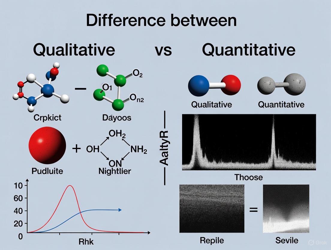
Spectroscopic analysis is a fundamental laboratory technique that involves the interaction of light with matter to determine the composition, concentration, and structural characteristics of samples [1]. This method encompasses various techniques utilizing different regions of the electromagnetic spectrum, each providing unique insights into molecular and elemental properties [2]. In pharmaceutical research and development, the choice between qualitative and quantitative analysis represents a critical first step in designing analytical strategies. Qualitative analysis identifies the presence or absence of particular chemical components in a sample, focusing on the "what" is present [3]. In contrast, quantitative analysis provides measurable, precise data regarding the concentration or mass of chemical components in a material, answering "how much" is present [3] [4]. These distinct yet complementary approaches form the foundation of analytical spectroscopy, enabling researchers to characterize compounds, monitor processes, and ensure product quality throughout the drug development lifecycle.
The importance of both analytical approaches spans across industries, with particular significance in pharmaceuticals, where accuracy in active ingredient composition ensures the safety and efficacy of drug products [3]. Environmental scientists use these analyses to monitor pollutants, while manufacturers rely on them for consistent product performance and regulatory compliance [3]. This technical guide explores the fundamental differences, methodologies, and applications of identification versus quantification in spectroscopic analysis, providing researchers and drug development professionals with a comprehensive framework for selecting and implementing appropriate analytical strategies.
Core Principles: Qualitative Versus Quantitative Analysis
Fundamental Differences in Objectives and Outputs
The distinction between qualitative and quantitative analysis represents a fundamental dichotomy in analytical spectroscopy, with each approach serving distinct yet complementary purposes in pharmaceutical research. Qualitative analysis is primarily exploratory and identification-focused, determining what elements or molecules are present in a sample without necessarily measuring their amounts [4]. This approach generates non-numerical data, such as spectral patterns or functional group identifications, that provide a chemical fingerprint of the sample [3] [5]. For example, infrared spectroscopy serves as a powerful qualitative tool for identifying functional groups in organic compounds through their characteristic absorption frequencies [3] [5].
In contrast, quantitative analysis provides numerical data that precisely define the concentration or mass of specific components within a sample [4]. This approach relies on the principle that the intensity of light absorbed or emitted by a substance is proportional to the number of atoms or molecules present in the analytical beam [1]. Quantitative methods require careful calibration and validation to ensure accuracy, precision, and reliability of the numerical results [6]. For instance, in pharmaceutical quality control, quantitative analysis verifies that active ingredients are present within specified concentration ranges to ensure drug efficacy and safety [3].
The relationship between these approaches is often sequential in drug development workflows. Qualitative analysis typically precedes quantitative assessment, with researchers first identifying the chemical constituents of a sample before determining their concentrations [3]. This systematic approach ensures that quantitative methods target the correct analytes and that appropriate reference standards are selected for accurate quantification.
Comparative Framework: Identification vs. Quantification
Table 1: Comparative Analysis of Qualitative and Quantitative Spectroscopic Methods
| Analytical Aspect | Qualitative Analysis | Quantitative Analysis |
|---|---|---|
| Primary Objective | Identify chemical components, functional groups, or structural features [3] | Determine concentration, mass, or abundance of specific analytes [4] |
| Nature of Output | Non-numerical: spectral patterns, presence/absence, chemical fingerprints [4] | Numerical: concentrations, mass values, quantitative ratios [4] |
| Common Techniques | FTIR, NMR, Raman, UV-Vis for functional group identification [3] [5] | AAS, ICP-MS, ICP-AES, UV-Vis spectroscopy with calibration [4] |
| Data Interpretation | Pattern recognition, spectral library matching, functional group analysis [7] [5] | Calibration curves, statistical analysis, reference to standards [6] |
| Typical Applications | Raw material identification, compound verification, structural elucidation [3] [8] | Assay development, impurity quantification, content uniformity [3] [6] |
| Accuracy Emphasis | Specificity and selectivity in identification | Precision, accuracy, and reproducibility of measurements |
| Speed of Analysis | Generally faster, more exploratory [3] | Often slower, requires careful calibration [3] |
Analytical Techniques and Methodologies
Qualitative Analysis Techniques and Protocols
Qualitative spectroscopic analysis employs a diverse array of techniques to identify chemical components based on their unique interactions with electromagnetic radiation. These methods leverage characteristic spectral patterns that serve as molecular fingerprints for compound identification.
Fourier Transform Infrared (FTIR) Spectroscopy has emerged as the preferred method for qualitative organic analysis due to its accuracy, sensitivity, and rapid data acquisition capabilities [5]. The experimental protocol involves several critical steps. First, sample preparation varies by physical state: solid samples may be ground with potassium bromide (KBr) and pressed into pellets, while liquid samples can be analyzed as thin films between salt plates. The prepared sample is then placed in the FTIR spectrometer, where it is exposed to infrared radiation across a range of wavenumbers (typically 4000-400 cm⁻¹). The instrument measures which frequencies are absorbed as the radiation passes through the sample, creating an absorption spectrum that reveals specific functional groups present in the molecule [5]. The resulting spectrum is divided into two diagnostically valuable regions: the functional group region (4000-1200 cm⁻¹) where characteristic stretching vibrations appear, and the fingerprint region (1200-400 cm⁻¹) that provides a unique pattern for compound verification [5]. For example, carbonyl groups (C=O) in ketones exhibit strong absorption at approximately 1710 cm⁻¹, while hydroxyl groups (O-H) in alcohols and carboxylic acids show broad bands around 3200-3600 cm⁻¹ [5].
Mass Spectrometry (MS) provides complementary qualitative information by separating ions based on their mass-to-charge ratio (m/z) [6]. The experimental workflow begins with sample ionization, commonly using electrospray ionization (ESI) or electron impact (EI) techniques to create gas-phase ions. These ions are then separated in a mass analyzer (such as quadrupole, time-of-flight, or ion trap systems) according to their m/z values [6]. Detection produces a mass spectrum that displays the relative abundance of ions at each m/z value, providing information about molecular weight and structural fragments. For small molecule identification, the molecular ion peak indicates the compound's molecular weight, while fragment peaks reveal structural characteristics through predictable breakdown patterns. In pharmaceutical applications, MS is particularly valuable for confirming the identity of drug compounds and detecting potential impurities or degradation products [6].
Advanced Chemometric Techniques for qualitative analysis include multivariate methods such as Principal Component Analysis (PCA) and Soft Independent Modeling of Class Analogies (SIMCA) [7]. These statistical approaches enhance the information extracted from complex spectral data sets. The PCA protocol begins with mean centering of the spectral data, followed by calculation of the covariance matrix to identify the largest sources of variance in the data set [7]. The resulting principal components form orthogonal vectors that represent the major patterns of variation, which can be visualized in score plots to identify clusters of similar samples and potential outliers [7]. SIMCA extends PCA by creating separate class models for different sample categories and classifying test samples based on their fit to these models using residual variance analysis [7]. These chemometric methods are particularly valuable in pharmaceutical development for raw material identification, batch-to-batch consistency monitoring, and detection of counterfeit products [7].
Quantitative Analysis Techniques and Protocols
Quantitative spectroscopic analysis requires meticulous method development, validation, and execution to generate reliable numerical data regarding analyte concentrations. These methods establish mathematical relationships between spectral signals and analyte quantities through carefully designed calibration procedures.
Ultraviolet-Visible (UV-Vis) Spectroscopy represents one of the most accessible and widely implemented quantitative techniques, particularly for compounds containing chromophores that absorb light in the UV or visible regions. The quantitative protocol begins with method development, which identifies the wavelength of maximum absorption (λmax) for the target analyte and verifies compliance with Beer-Lambert law through linearity studies [2] [9]. Sample preparation typically involves dissolving the analyte in a suitable solvent that does not interfere with measurements, followed by preparation of a standard series with known concentrations spanning the expected range of the samples [9]. The spectrophotometer is zeroed using a blank solution containing all components except the analyte, after which absorbance measurements are collected for all standards and unknown samples at the predetermined λmax [9]. Data processing involves constructing a calibration curve by plotting absorbance versus concentration for the standard series, followed by linear regression analysis to establish the mathematical relationship (A = εbc, where A is absorbance, ε is molar absorptivity, b is path length, and c is concentration) [9]. Unknown concentrations are then calculated by interpolating their absorbance values on the calibration curve [9]. In pharmaceutical applications, this technique is routinely employed for drug assay and content uniformity testing, with validation parameters including accuracy, precision, linearity, range, and specificity [9].
Atomic Absorption Spectroscopy (AAS) provides highly sensitive quantitative analysis of metal elements in pharmaceutical materials, particularly for catalyst residues or elemental impurities. The experimental methodology involves several critical steps [4] [9]. Sample preparation typically requires digestion of organic matrices using concentrated acids to release metal ions into solution, followed by appropriate dilution to fall within the instrument's linear range [9]. The instrumental analysis utilizes a hollow cathode lamp specific to the target element to generate characteristic wavelengths that the element will absorb [9]. The sample solution is aspirated into a flame (air-acetylene or nitrous oxide-acetylene) or electrothermal atomizer that converts the ions into free ground-state atoms [9]. Measurement occurs when light from the element-specific lamp passes through the atomized sample, with the amount of light absorbed being proportional to the concentration of ground-state atoms in the optical path [9]. Quantification relies on calibration with matrix-matched standard solutions to account for potential interferences, with detection limits typically in the parts-per-million to parts-per-billion range depending on the element and instrumentation [4] [9]. Pharmaceutical applications include quantification of metal catalysts in active pharmaceutical ingredients and compliance testing for elemental impurities according to regulatory guidelines such as ICH Q3D [9].
Quantitative Mass Spectrometry (MS) has emerged as a powerful technique for quantifying analytes in complex matrices, particularly in bioanalytical applications such as pharmacokinetic studies [6]. The experimental workflow incorporates several critical steps to address the technical challenges of quantitative MS analysis. Sample preparation often involves extraction techniques such as protein precipitation, liquid-liquid extraction, or solid-phase extraction to isolate analytes from biological matrices and reduce ion suppression effects [6]. Chromatographic separation using liquid chromatography (LC) or gas chromatography (GC) is typically incorporated prior to MS detection to separate analytes from matrix components that could cause interference [6]. Mass spectrometric detection employs selective reaction monitoring (SRM) or multiple reaction monitoring (MRM) modes on triple quadrupole instruments to achieve high specificity and sensitivity [6]. Stable isotope-labeled internal standards (SIL-IS), which are chemically identical to the analytes but contain heavier isotopes (²H, ¹³C, ¹⁵N), are added to all samples and standards to correct for variability in sample preparation, ionization efficiency, and matrix effects [6]. Calibration standards and quality control samples prepared in the same matrix as the study samples are analyzed alongside unknowns to establish the quantitative relationship between analyte concentration and detector response [6]. Validation parameters for quantitative MS methods include specificity, sensitivity, accuracy, precision, matrix effects, and stability to ensure reliable performance [6].
Table 2: Quantitative Techniques and Their Pharmaceutical Applications
| Technique | Analytical Principle | Quantifiable Parameters | Pharmaceutical Applications | Typical Sensitivity Range |
|---|---|---|---|---|
| UV-Vis Spectroscopy | Absorption of UV/visible light by chromophores [2] | Concentration of light-absorbing compounds [9] | Drug assay, content uniformity, dissolution testing [9] | 10⁻⁴ to 10⁻⁶ M [9] |
| Atomic Absorption Spectroscopy | Absorption of element-specific radiation by ground-state atoms [4] [9] | Concentration of metal elements [4] | Catalyst residues, elemental impurities [9] | ppm to ppb [4] [9] |
| ICP-MS | Ionization of elements in plasma and mass separation [4] | Concentration of elements, isotopic ratios [4] | Elemental impurities per ICH Q3D, trace metal analysis [4] | ppb to ppt [4] |
| Quantitative LC-MS/MS | Chromatographic separation followed by mass detection [6] | Concentration of small molecules, peptides, biomarkers [6] | Pharmacokinetics, bioequivalence, metabolite quantification [6] | pg/mL to ng/mL [6] |
| Fluorescence Spectroscopy | Emission of light after excitation at specific wavelength [1] | Concentration of fluorescent compounds [1] | High-sensitivity assays, protein quantification [1] | 10⁻⁸ to 10⁻¹⁰ M [1] |
Experimental Design and Workflow Integration
Strategic Selection Framework
The decision between qualitative and quantitative analytical approaches requires careful consideration of research objectives, sample characteristics, and regulatory requirements. A systematic framework ensures appropriate method selection aligned with project goals throughout the drug development lifecycle.
Diagram 1: Analytical Method Selection Framework
The analytical strategy begins with precisely defining the research question. Qualitative analysis is appropriate when the goal is compound identification, structural elucidation, impurity profiling, or material classification [3]. For example, during early drug discovery, qualitative techniques identify potential drug candidates and characterize their chemical structures [3] [8]. When reference standards are unavailable or when the chemical identity of a sample is unknown, qualitative methods provide the necessary information to establish identity [3]. Quantitative analysis becomes essential when numerical data are required to support specific claims about composition, potency, or purity [6]. This includes drug assay determination, impurity quantification, content uniformity testing, and dissolution profile characterization [3] [6]. Regulatory submissions typically require validated quantitative methods for critical quality attributes [7] [6]. In many cases, a sequential approach employing both qualitative and quantitative techniques provides the most comprehensive analytical solution, such as identifying an impurity qualitatively before developing a quantitative method to control its level in the drug product [3].
The Scientist's Toolkit: Essential Research Reagent Solutions
Table 3: Essential Research Reagents for Spectroscopic Analysis
| Reagent/Category | Function/Purpose | Application Context |
|---|---|---|
| FTIR Grade KBr | Matrix for solid sample preparation; transparent to IR radiation [5] | FTIR sample preparation for solid compounds [5] |
| Deuterated Solvents (CDCl₃, DMSO-d₆) | NMR solvents providing deuterium lock signal; minimize solvent interference [1] | NMR spectroscopy for structural elucidation [1] |
| HPLC/MS Grade Solvents | High purity solvents for LC-MS minimizing background interference [6] | Mobile phase preparation in quantitative LC-MS [6] |
| Stable Isotope-Labeled Internal Standards | Correction for variability in sample preparation and ionization [6] | Quantitative MS for pharmacokinetic studies [6] |
| Certified Reference Standards | Calibration with known purity and concentration [6] [4] | Quantitative method calibration and validation [6] [4] |
| Matrix-Matched Standards | Standards prepared in same matrix as samples to correct for matrix effects [6] | Quantitative analysis in complex biological matrices [6] |
The distinction between identification and quantification represents a fundamental paradigm in analytical spectroscopy, with each approach serving distinct yet complementary roles in pharmaceutical research and development. Qualitative analysis provides the essential foundation for understanding chemical composition, identifying unknown compounds, and elucidating molecular structures through techniques such as FTIR, NMR, and mass spectrometry [3] [5]. Quantitative analysis builds upon this foundation to deliver precise numerical data regarding analyte concentrations, enabling critical assessments of potency, purity, and quality through validated methods such as UV-Vis spectroscopy, AAS, and LC-MS/MS [6] [9].
The strategic selection between these approaches depends fundamentally on the analytical goal, with qualitative methods answering "what is present" and quantitative methods determining "how much is present" [3] [4]. In contemporary drug development, the integration of both approaches throughout the product lifecycle—from discovery through commercial manufacturing—provides the comprehensive analytical understanding necessary to ensure drug safety, efficacy, and quality. As spectroscopic technologies continue to advance, with improvements in sensitivity, resolution, and data processing capabilities, the synergy between qualitative and quantitative analysis will further enhance their collective impact on pharmaceutical innovation and patient care.
Key Principles of Qualitative Spectroscopic Analysis
Qualitative spectroscopic analysis is a fundamental scientific discipline concerned with identifying the chemical composition and molecular structures present in a sample. Framed within a broader thesis on spectroscopic research, it serves a purpose distinct from, yet complementary to, quantitative analysis. While quantitative analysis seeks to answer "how much" of a component is present by providing precise numerical data on concentration, qualitative analysis answers "what" is present by identifying substances based on their unique spectral fingerprints [3]. This identification of components—whether elements, functional groups, or entire molecules—is the essential first step in analytical characterization, upon which meaningful quantitative assessment can be built [1].
The foundation of all qualitative spectroscopy is the interaction of light (electromagnetic radiation) with matter. When a sample is exposed to light, it can absorb, emit, or scatter energy at specific wavelengths that are characteristic of its atomic and molecular constituents [10]. The resulting spectrum is a plot of the response versus energy or wavelength, serving as a unique identifier, much like a molecular "fingerprint" [2] [11]. This non-destructive technique is widely applied across fields including pharmaceuticals, environmental monitoring, food safety, and biomedical diagnostics [1] [12].
Theoretical Foundations: The Electromagnetic Spectrum and Molecular Transitions
The choice of spectroscopic technique is determined by the region of the electromagnetic spectrum employed, as different regions probe distinct types of molecular transitions and provide different categories of qualitative information.
Table 1: Spectroscopic Regions and Their Qualitative Information Content
| Spectral Region | Wavelength Range | Molecular Transition | Primary Qualitative Information | Example Techniques |
|---|---|---|---|---|
| Ultraviolet (UV) | 190–360 nm [2] | Electronic transitions of electrons in double/triple bonds and non-bonding orbitals [2] | Presence of chromophores (e.g., carbonyls, nitriles) [2] | UV Spectroscopy |
| Visible (Vis) | 360–780 nm [2] | Electronic transitions in colored compounds/pigments [2] | Color measurement, coordination compound identity | Visible Spectroscopy |
| Near-Infrared (NIR) | 700–2500 nm [11] | Overtone and combination bands of fundamental vibrations (e.g., C-H, O-H, N-H) [2] | Identification of broad functional groups in complex matrices (e.g., polymers, food) [2] | NIR Spectroscopy |
| Infrared (IR) | 2500–50,000 nm [11] | Fundamental molecular vibrations (stretching and bending) [11] | Identification of specific functional groups and molecular structure [2] [1] | FTIR, IR Spectroscopy |
| Raman | Varies (often 100-3500 cm⁻¹) | Inelastic scattering due to molecular vibrations and rotations [2] | Complementary to IR; effective for symmetric bonds (e.g., C=C, S-S) and aqueous samples [2] | Raman Spectroscopy |
The information contained in each region is directly tied to the energy of the photons. Ultraviolet and visible radiation, with higher energy, promotes electrons to higher energy states, while lower-energy infrared radiation causes bonds to vibrate [11]. The quantized nature of these energy states means that the absorbed or emitted wavelengths are highly specific to the chemical species involved, forming the fundamental basis for qualitative identification [11] [1].
Key Methodological Principles
Spectral Interpretation and Fingerprinting
The most direct principle of qualitative analysis is spectral fingerprinting. This involves comparing the entire spectrum of an unknown sample to a library of reference spectra from known compounds [7]. A high degree of correlation between the unknown and a reference spectrum confirms the identity of the material. Techniques like Wavelength Correlation (WC) and Euclidean Distance (ED) are simple, robust mathematical tools used for this comparison. A correlation value near 1.0 or a small Euclidean distance value indicates a strong match [7]. This method is particularly common for raw material identification in pharmaceutical manufacturing where a quick, definitive identity check is required [7].
The Role of Chemometrics in Qualitative Analysis
Modern qualitative analysis, especially with complex samples or techniques like NIR and Raman, heavily relies on chemometrics—the use of statistical methods to extract chemical information from multivariate data [7] [13]. These methods transform spectral data to uncover latent patterns related to sample class or identity.
- Principal Component Analysis (PCA): An unsupervised technique used for exploratory data analysis and outlier detection [7] [13]. PCA reduces the dimensionality of complex spectral data, revealing the dominant sources of variation. Samples with similar composition will cluster together in a scores plot, while anomalous samples will appear as outliers. This allows scientists to visualize natural groupings in their data without prior knowledge of sample classes [7].
- Soft Independent Modeling of Class Analogy (SIMCA): A supervised classification method that builds a separate PCA model for each predefined class of samples (e.g., olive oil, corn oil) [7]. An unknown sample is then compared to each class model, and its classification is based on how well it fits each model, quantified by its distance to the model (DmodX) [7]. SIMCA is more sensitive than simple PCA for group classification.
- Partial Least Squares-Discriminant Analysis (PLS-DA): A highly sensitive supervised method that finds the relationship between spectral data (X) and a categorical class membership matrix (Y) [14] [7]. It rotates latent variables to not only capture variance in X but also to maximize separation between predefined classes. PLS-DA was used, for instance, to achieve 100% accuracy in identifying the animal origin (cow, goat, or sheep) of milk in yogurt [14].
- Machine Learning and AI: Advanced algorithms are increasingly being integrated into spectroscopic analysis. Support Vector Machines (SVM), Random Forest (RF), and Deep Learning models can handle complex, non-linear relationships in spectral data, further enhancing the power and accuracy of qualitative classification [13].
Experimental Protocols and Workflows
General Workflow for Qualitative Spectroscopic Analysis
The following diagram outlines a standard workflow for conducting a qualitative spectroscopic analysis, from sample preparation to final interpretation.
Protocol: Identification of Milk Origin in Yogurt Using Vis-NIR and PLS-DA
This specific protocol, derived from a published study, demonstrates the application of chemometrics to a real-world qualitative problem [14].
- 1. Objective: To predict the animal origin (cow, goat, or sheep) of milk used in yogurt production as a means of food authentication.
- 2. Sample Preparation:
- Prepare yogurt samples from known milk sources (cow, goat, sheep) under controlled conditions.
- Ensure a sufficient number of batches for each class to build a robust model (training set) and an independent set for validation (test set).
- Present samples to the spectrometer in a consistent manner, using a suitable transparent container or reflectance probe.
- 3. Instrumentation and Data Acquisition:
- Technique: Visible and Near-Infrared (Vis-NIR) Spectroscopy.
- Device: A spectrophotometer capable of acquiring spectra in the 400–2500 nm range.
- Parameters: Acquire multiple spectra per sample to account for heterogeneity and average them to improve the signal-to-noise ratio.
- 4. Data Pre-processing:
- The study found the optimal range for species identification to be 400–600 nm [14].
- Apply spectral pre-processing techniques to the data from this range. Common methods include:
- Scatter Correction (e.g., Standard Normal Variate, Multiplicative Scatter Correction) to reduce light scattering effects.
- Smoothing to reduce high-frequency noise.
- Derivative (e.g., 1st or 2nd derivative) to resolve overlapping peaks and remove baseline offsets.
- 5. Chemometric Modeling and Classification:
- Algorithm: Partial Least Squares-Discriminant Analysis (PLS-DA).
- Process:
- Build a PLS-DA model using the pre-processed training spectra. The model learns the spectral patterns that are characteristic of each milk class.
- Use the model to predict the class of the validation samples.
- Assess model performance using a confusion matrix and calculate the accuracy. The referenced study achieved 100% accuracy in distinguishing the three milk types [14].
Protocol: Discriminating Oils using Mid-IR and PCA/SIMCA
- 1. Objective: To discriminate between different types of oils (e.g., olive, corn, safflower) based on their Mid-Infrared spectra.
- 2. Sample Preparation:
- Use pure, undiluted oil samples. A small drop between two infrared-transparent windows (e.g., KBr) is sufficient for transmission measurement.
- 3. Instrumentation and Data Acquisition:
- Technique: Mid-Infrared (IR) Spectroscopy.
- Spectral Range: 4000 - 400 cm⁻¹.
- 4. Data Pre-processing:
- Apply standard pre-processing such as atmospheric suppression (to remove CO₂ and water vapor bands) and vector normalization.
- 5. Chemometric Modeling and Classification:
- Exploratory Analysis: Perform PCA on the spectral data. A scores plot (PC1 vs. PC2) will typically show distinct clustering of samples by oil type, allowing for visual identification and outlier detection [7].
- Classification: Apply SIMCA by developing a separate PCA model for each oil type. A Cooman's plot can then be used to visualize whether test samples belong to a specific class or are outliers, providing a statistical basis for authentication [7].
The Scientist's Toolkit: Essential Reagents and Materials
Table 2: Key Research Reagents and Materials for Qualitative Spectroscopy
| Item | Function in Qualitative Analysis |
|---|---|
| Certified Reference Materials (CRMs) | Provides known spectral fingerprints for library building and instrument calibration; essential for method validation [15]. |
| Infrared-Transparent Windows (e.g., KBr, NaCl) | Used to hold samples in transmission IR spectroscopy; must be transparent in the IR region of interest [1]. |
| Solvents (e.g., CDCl₃ for NMR, ACN for UV) | Dissolve solid samples for analysis; must be spectroscopically pure to avoid interfering signals in the analytical region. |
| Chemometric Software | Provides algorithms (PCA, SIMCA, PLS-DA, Machine Learning) for processing, modeling, and interpreting complex spectral data [7] [13]. |
Advanced Concepts: The Integration of Artificial Intelligence
The field of qualitative spectroscopy is being transformed by Artificial Intelligence (AI) and Machine Learning (ML). While traditional chemometrics remains vital, AI frameworks automate feature extraction and enable the modeling of complex, non-linear relationships in spectral data [13].
- Deep Learning (DL): A subset of ML using multi-layered neural networks, Convolutional Neural Networks (CNNs) can automatically learn hierarchical features from raw or minimally preprocessed spectra, often outperforming traditional linear methods [13].
- Generative AI (GenAI): Can create synthetic spectral data that mimics real samples. This is used to balance datasets, augment training data, and enhance the robustness of qualitative models, especially when real data is scarce [13].
- Explainable AI (XAI): As AI models can be "black boxes," XAI frameworks (e.g., SHAP, Grad-CAM) are increasingly important. They help identify which wavelengths the model found most informative for classification, preserving the chemical interpretability that is central to spectroscopy [13].
The key principles of qualitative spectroscopic analysis—from fundamental spectral fingerprinting to advanced chemometric and AI-driven classification—provide powerful tools for identifying chemical substances. By leveraging the unique interaction of light with matter across the electromagnetic spectrum and applying sophisticated data modeling techniques, researchers can confidently answer the critical question of "what is present?" This foundational capability supports a vast range of scientific and industrial activities, ensuring product authenticity, safeguarding public health, and driving research discovery. The ongoing integration of artificial intelligence promises to further enhance the sensitivity, speed, and scope of qualitative spectral analysis.
Key Principles of Quantitative Spectroscopic Analysis
Spectroscopic analysis serves as a fundamental tool in chemical science, operating primarily in two distinct yet complementary modes: qualitative and quantitative analysis. Qualitative analysis focuses on identifying the chemical composition of a sample—answering the question "What is present?" by identifying specific elements, functional groups, or molecules based on their characteristic spectral patterns [3] [1]. In contrast, quantitative analysis determines the concentration or absolute amount of specific components within a sample, answering "How much is present?" by measuring the relationship between the intensity of the spectroscopic signal and the analyte concentration [3] [1].
This guide details the core principles, methodologies, and applications of quantitative spectroscopic analysis, providing researchers and drug development professionals with a technical foundation for precise concentration measurement across various spectroscopic techniques.
Core Principles of Quantitative Spectroscopic Analysis
The foundation of quantitative spectroscopy rests on two well-established physical laws and the careful management of experimental parameters to ensure data accuracy.
The Beer-Lambert Law
The Beer-Lambert law forms the cornerstone of quantitative absorption spectroscopy (including UV-Vis, IR, NIR) [11]. It states that the absorbance of light by a solution is directly proportional to the concentration of the absorbing species and the pathlength of light through the sample. The mathematical expression is:
A = εlc
Where:
- A is the measured absorbance (unitless)
- ε is the molar absorptivity or extinction coefficient (L·mol⁻¹·cm⁻¹)
- l is the pathlength of the sample cell (cm)
- c is the concentration of the analyte (mol·L⁻¹)
This linear relationship allows for the determination of an unknown concentration by measuring its absorbance, provided the molar absorptivity and pathlength are known [2] [11].
Signal-to-Concentration Relationship
In emission spectroscopy (e.g., fluorescence, ICP-OES) and other techniques like Raman and NMR, the intensity of the emitted or scattered signal is directly proportional to the number of atoms or molecules producing that signal [1]. This principle enables quantification without a direct absorption measurement. The general relationship is:
I = kc
Where:
- I is the measured signal intensity
- k is a proportionality constant dependent on the instrument and analyte
- c is the concentration of the analyte
Calibration and Linear Dynamic Range
Quantitative analysis requires constructing a calibration curve by measuring the spectroscopic response (e.g., absorbance, intensity) for a series of standard solutions with known concentrations [1]. This curve establishes the working relationship between signal and concentration for the specific analyte and instrument. The linear dynamic range is the concentration interval over which this relationship remains linear, defining the valid quantitative range of the method.
Sensitivity and Limit of Detection
- Sensitivity refers to the ability of a method to distinguish between small differences in concentration, often reflected in the slope of the calibration curve.
- Limit of Detection (LOD) is the lowest concentration that can be detected, though not necessarily quantified, with a specified degree of confidence.
- Limit of Quantification (LOQ) is the lowest concentration that can be quantitatively determined with acceptable precision and accuracy.
Advanced techniques can achieve detection limits as low as parts per billion under optimal conditions [1].
Experimental Design and Methodologies
Robust quantitative results require carefully designed experiments to account for potential interferences and matrix effects.
General Quantitative Workflow
The following diagram illustrates the standard workflow for a quantitative spectroscopic analysis, from sample preparation to final concentration calculation.
Detailed Protocol: Quantitative Mass Spectrometry Imaging of Neurotransmitters
A recent (2025) advanced protocol for quantifying neurotransmitters in rodent brain tissue using MALDI Mass Spectrometry Imaging (MALDI-MSI) highlights strategies to overcome matrix effects in complex samples [16].
1. Problem: Precise quantitation in spatially heterogeneous samples like brain tissue is hampered by varying ionization efficiencies and localized matrix effects, which can suppress the analytical signal and introduce significant error [16].
2. Solution: Employ a standard addition method with homogeneous spraying of stable isotope-labeled (SIL) internal standards onto tissue sections to normalize signals and account for spatial variability [16].
3. Experimental Workflow:
4. Key Steps:
- Tissue Preparation: Sagittal brain tissue sections (12 µm thickness) are placed on ITO-coated slides [16].
- Internal Standard Application: SIL analogues (e.g., DA-d₄, NE-d₆) are homogeneously sprayed over tissue sections in six passes using a robotic sprayer (TM-sprayer) for normalization [16].
- Calibration Standard Application: Different concentrations of calibration standards (e.g., dopamine, norepinephrine) are sprayed in a quantitative manner over consecutive tissue sections [16].
- Matrix Application & Data Acquisition: The derivatizing matrix FMP-10 is applied. MALDI-MSI data is acquired using a FTICR mass spectrometer in positive ion mode (e.g., over m/z 150–1500) [16].
- Quantitation: Signal intensities for neurotransmitters and metabolites are extracted from regions of interest. A calibration curve is plotted for each analyte, and the endogenous concentration is determined from the x-intercept of the trend line [16].
5. Outcome: This standard addition approach provided strong linearity (R² > 0.99) and results comparable to HPLC-ECD, significantly enhancing quantitation accuracy in a complex tissue environment [16].
Data Presentation and Analysis
Quantitative Data Tables for Spectroscopic Analysis
Table 1: Characteristic Infrared Absorption Frequencies for Common Functional Groups [17]
| Approximate Frequency (cm⁻¹) | Bond Vibration | Functional Group | Notes |
|---|---|---|---|
| 1800-1600 | C=O stretch | Carbonyl | Strong peak; lower frequency (1650-1550) if attached to O or N [17] |
| 3500-3200 | O-H stretch | Alcohol, Carboxylic Acid | Broad, round; much broader if in carboxylic acid [17] |
| 3400-3300 | N-H stretch | Amine | Weak, triangular shape [17] |
| 2250 | C≡N stretch | Nitrile | Medium intensity [17] |
| 2250-2100 | C≡C stretch | Alkyne | Weak-medium intensity [17] |
| 3100-3000 | =C-H stretch | Alkene (sp² C-H) | Weak-medium intensity [17] |
| 3000-2900 | -C-H stretch | Alkane (sp³ C-H) | Weak-medium intensity [17] |
Table 2: Electromagnetic Spectrum Regions Used in Quantitative Analysis
| Spectral Region | Wavelength Range | Primary Quantitative Application | Typical Samples |
|---|---|---|---|
| Ultraviolet (UV) | 190 - 360 nm [2] | Concentration of chromophores [2] | Pharmaceutical compounds (HPLC detection) [2] |
| Visible (Vis) | 360 - 780 nm [2] | Colorimetric analysis, dye concentration [2] [1] | Blood samples (clinical analyzers) [1] |
| Near-Infrared (NIR) | 700 - 2500 nm [11] | Multicomponent analysis (e.g., moisture, proteins) [2] | Agricultural products, food, pharmaceuticals [2] |
| Infrared (IR) | 2500 - 50,000 nm [11] | Functional group concentration, polymer analysis [2] | Organic compounds, polymers [2] |
| Raman | Varies (laser dependent) | Aqueous samples, symmetric vibrations [2] | Biological samples, inorganic crystals [2] |
The Scientist's Toolkit: Essential Research Reagents and Materials
Table 3: Key Reagent Solutions for Quantitative Spectroscopic Experiments
| Reagent / Material | Function in Quantitative Analysis | Example Application |
|---|---|---|
| Stable Isotope-Labeled (SIL) Internal Standards | Correct for variability in sample preparation and ionization efficiency; enable standard addition method [16]. | Quantification of dopamine-d₄ in brain tissue via MALDI-MSI [16]. |
| Calibration Standards (Analytes of Known Purity) | Establish the primary calibration curve for converting instrument response to concentration [1]. | Creating a standard curve for glucose concentration in serum using UV-Vis spectroscopy. |
| Derivatizing Agents (e.g., FMP-10) | Chemically tag target analytes to enhance their detection sensitivity and specificity in the mass spectrometer [16]. | Improving the signal for neurotransmitters in MALDI-MSI [16]. |
| Matrix Compounds (e.g., for MALDI) | Absorb laser energy and facilitate soft desorption/ionization of the sample for mass spectrometric analysis [16]. | Enabling ionization of large biomolecules in MALDI-MS. |
| Spectroscopic Solvents (e.g., HPLC-grade) | Dissolve samples and standards without introducing interfering spectral signals or contaminants. | Preparing samples for UV-Vis or IR spectroscopy to ensure a clean baseline. |
| Buffer Solutions | Maintain constant pH and ionic strength to ensure consistent analyte form and spectroscopic response. | Stabilizing protein conformations for fluorescence quantification. |
Applications in Research and Industry
Quantitative spectroscopy is indispensable in numerous fields due to its precision, sensitivity, and often non-destructive nature.
- Pharmaceutical Development and Quality Control: Used extensively to determine active ingredient composition, ensure safety and efficacy, and monitor reactions [3]. UV-Vis detectors are routinely used as a final check in HPLC systems before drug product release [2].
- Clinical Diagnostics: Automated clinical chemistry analyzers perform "chem twenty" blood tests using visible and UV absorption spectroscopy to quantify blood components like glucose, cholesterol, and enzymes, providing critical data for patient diagnosis and treatment monitoring [1].
- Industrial Process and Quality Control: Provides rapid, quantitative feedback for regulating manufacturing processes. Applications include determining fat content in peanut butter, sugar in fruit juices, and carbon dioxide in beverages using NIR and IR spectroscopy [2] [1].
- Environmental and Food Monitoring: Used to detect and quantify contaminants, additives, and constituents at levels ranging from percentage down to parts per billion [1] [12]. Infrared analysis can identify and measure compounds like formaldehyde and nitrogen oxides in engine exhaust [1].
The Synergistic Relationship in the Analytical Workflow
In the fields of analytical chemistry and pharmaceutical development, the journey from an unknown sample to a fully characterized and quantified substance is a structured process that relies heavily on the complementary strengths of qualitative and quantitative analysis. Qualitative analysis identifies the presence or absence of particular chemical components in a sample, focusing on the "what" [3]. Quantitative analysis, in contrast, provides measurable, precise data regarding the concentration or amount of these components, answering the question of "how much" [3]. Spectroscopic methods form the backbone of this analytical workflow, providing the tools for both identification and measurement. This guide explores the synergistic relationship between these two approaches, detailing how their integrated application ensures accuracy, efficiency, and reliability in research and drug development.
Fundamental Concepts: Qualitative and Quantitative Analysis
Qualitative Chemical Analysis
The primary objective of qualitative analysis is the identification of chemical substances or functional groups within a sample [3] [18]. It is an exploratory process, often used in the initial stages of research or for troubleshooting when unknown substances affect product consistency or function [3].
Common Qualitative Techniques and Applications:
- Infrared (IR) Spectroscopy: Identifies functional groups based on their characteristic fundamental molecular vibrations [3] [2]. For example, the carbonyl group (C=O) in a ketone exhibits a strong absorption between 1800-1600 cm⁻¹ [17].
- Raman Spectroscopy: Complementary to IR, it is particularly useful for characterizing symmetric vibrations and is ideal for aqueous samples as water is a weak scatterer [2].
- Nuclear Magnetic Resonance (NMR) Spectroscopy: Provides detailed information on the carbon-hydrogen framework of a molecule, enabling full structural elucidation [3].
Quantitative Chemical Analysis
Once components are identified, quantitative analysis determines their concentration. This method is indispensable for determining exact ratios, evaluating regulatory compliance, and standardizing formulations where precision is critical [3].
Common Quantitative Techniques and Applications:
- Ultraviolet-Visible (UV-Vis) Spectroscopy: Measures the absorption of light by a sample at specific wavelengths to determine analyte concentration, often via Beer-Lambert's Law [2] [9]. It is frequently used as a detector in High-Performance Liquid Chromatography (HPLC) [2].
- Atomic Absorption Spectroscopy (AAS): Used for determining the concentration of specific metal elements in a sample [19].
- Inductively Coupled Plasma Mass Spectrometry (ICP-MS): Provides highly sensitive multi-elemental quantitative data [19].
- Titration: A classical method that measures the volume of a reagent required to complete a reaction with the analyte [3].
The Synergistic Analytical Workflow
The true power of analytical science is realized when qualitative and quantitative analyses are integrated into a single, cohesive workflow. This synergy creates a logical progression from discovery to measurement, where each step informs the next.
The following diagram illustrates this iterative and complementary relationship:
Workflow Description
- Initial Qualitative Screening: The workflow begins with an unknown sample. Qualitative techniques, such as IR or Raman spectroscopy, are employed to gain a broad overview and identify potential components or impurities [3]. For instance, FTIR can rapidly characterize complex mixtures in resins or acids [3].
- Hypothesis Formulation: The data from the qualitative analysis allows researchers to formulate a hypothesis about the sample's composition—what functional groups, molecules, or elements are present.
- Quantitative Measurement: With the components identified, a targeted quantitative method is developed and applied. This step provides the precise numerical data required for decision-making, such as the exact concentration of an active pharmaceutical ingredient (API) to ensure safety and efficacy [3].
- Result Validation and Feedback Loop: The final result is a fully characterized sample. However, the workflow is often iterative. An anomaly in quantitative results (e.g., lower-than-expected yield) may trigger a new round of qualitative analysis to identify unknown contaminants or degradation products, thus closing the loop and starting the cycle anew [3].
Detailed Methodologies and Data Interpretation
Experimental Protocols for Key Techniques
Protocol 1: Qualitative Identification of Functional Groups using FTIR Spectroscopy
- Sample Preparation:
- Solid Samples: A small amount (~1-2 mg) of the solid is finely ground and mixed with dry potassium bromide (KBr, ~100-200 mg). This mixture is compressed under high pressure to form a transparent pellet. Alternatively, for ATR (Attenuated Total Reflectance) sampling, a solid can be placed directly onto the crystal and clamped for measurement [17] [18].
- Liquid Samples: A drop of the neat liquid can be sandwiched between two salt plates (e.g., NaCl or KBr). For volatile liquids, a sealed liquid cell is used [18].
- Data Acquisition: The prepared sample is placed in the FTIR spectrometer. A background spectrum is first collected. The sample spectrum is then acquired over a range of 4000-400 cm⁻¹, typically averaging 16-32 scans at a resolution of 4 cm⁻¹ to ensure a high signal-to-noise ratio [18].
- Data Interpretation: The resulting spectrum is analyzed by comparing the observed absorption bands to known characteristic group frequencies (see Table 1).
Protocol 2: Quantitative Analysis of an Active Ingredient using UV-Vis Spectroscopy
- Calibration Curve Method:
- Standard Solution Preparation: A stock solution of the pure analyte (reference standard) is prepared. A series of standard solutions of known concentration (e.g., 5-7 points) are made by serial dilution.
- Absorbance Measurement: The absorbance of each standard solution is measured at the wavelength of maximum absorption (λₘₐₓ), previously determined from a qualitative UV-Vis scan.
- Calibration Plot: A graph of absorbance versus concentration is plotted. The data should yield a linear relationship, conforming to the Beer-Lambert Law [9].
- Sample Analysis: The absorbance of the unknown sample solution is measured under identical conditions. The concentration is determined by interpolating the sample absorbance on the calibration curve.
Data Presentation and Interpretation
Table 1: Characteristic Infrared Absorption Frequencies of Common Functional Groups (Qualitative Analysis) [17]
| Approximate Frequency (cm⁻¹) | Bond Vibration | Functional Group | Notes |
|---|---|---|---|
| 3500 - 3200 | O-H stretching | Alcohols, Carboxylic Acids | Broad, round; broader for acids |
| 3400-3300 | N-H stretching | Primary, Secondary Amines | Weak, triangular shape |
| ~2250 | C≡N stretching | Nitriles | Medium intensity, sharp |
| 1800-1600 | C=O stretching | Carbonyls (Ketones, Aldehydes) | Strong, very characteristic |
| 1650-1450 | C=C stretching | Alkenes, Aromatics | Weak-medium; pattern indicates substitution |
Table 2: Comparison of Common Spectroscopic Techniques for Qualitative and Quantitative Analysis [3] [2] [19]
| Technique | Primary Qualitative Application | Primary Quantitative Application | Key Strengths |
|---|---|---|---|
| UV-Vis Spectroscopy | Identification of chromophores (e.g., conjugated systems) | Concentration measurement of light-absorbing species | Simple, fast, highly quantitative |
| IR Spectroscopy | Identification of functional groups and molecular fingerprints | Limited quantitative use (e.g., polymer cure) | Excellent for identification, rich in structural information |
| Atomic Emission Spectroscopy | Elemental identification | Multi-element concentration measurement | Wide dynamic range, suitable for trace metal analysis |
| Raman Spectroscopy | Identification of symmetrical vibrations, aqueous samples | Concentration measurement (often with chemometrics) | Complementary to IR, minimal sample prep |
| NMR Spectroscopy | Full molecular structure elucidation | Determining purity, isomeric ratio, quantitative NMR (qNMR) | Extremely powerful for structure determination |
The Scientist's Toolkit: Essential Research Reagents and Materials
Table 3: Key Research Reagent Solutions and Essential Materials
| Item | Function / Application |
|---|---|
| Potassium Bromide (KBr) | Used for preparing transparent pellets for FTIR analysis of solid samples [18]. |
| Deuterated Solvents (e.g., CDCl₃, D₂O) | Solvents for NMR spectroscopy that do not produce interfering proton signals [3]. |
| Reference Standards (Certified) | High-purity materials of known identity and concentration used for calibration in quantitative analyses (e.g., UV-Vis, HPLC) [3]. |
| Salt Plates (NaCl, KBr) | Windows for liquid sample holders in IR spectroscopy; transparent in the mid-IR region [18]. |
| Buffer Solutions | Used to maintain a constant pH during spectroscopic analysis, which is critical for the stability and accurate measurement of many analytes, particularly in UV-Vis and fluorescence spectroscopy. |
| Internal Standards | A known compound added in a constant amount to all samples and standards in quantitative analyses (e.g., ICP-MS, GC) to correct for variability and improve accuracy. |
The analytical workflow is not a choice between qualitative or quantitative analysis but a strategic integration of both. Qualitative spectroscopy provides the essential map of molecular identity, while quantitative spectroscopy delivers the precise measurements required for validation, standardization, and compliance. This synergistic relationship—moving from the "what" to the "how much"—is fundamental to progress in pharmaceutical development, materials science, and environmental monitoring. By leveraging their unique benefits in a sequential and iterative manner, researchers and scientists can maintain the highest quality standards, accelerate innovation, and ensure the safety and efficacy of final products.
Spectroscopic techniques form the cornerstone of modern analytical chemistry, providing powerful tools for determining the structure, identity, and quantity of chemical substances. These methods are fundamentally categorized into two distinct research approaches: qualitative analysis, which identifies the presence or absence of particular chemical components in a sample (answering "what is it?"), and quantitative analysis, which provides measurable, precise data about the concentration or amount of these components (answering "how much is there?") [3]. This distinction is crucial across industries—from pharmaceuticals where they ensure drug safety and efficacy, to environmental monitoring where they detect and quantify pollutants [3].
The global molecular spectroscopy market, valued at $3.9 billion in 2024 and projected to reach $6.4 billion by 2034, reflects the critical importance of these techniques [20]. This growth is driven by increasing demand for advanced analytical tools in drug development, quality control, and environmental testing [20]. This technical guide provides an in-depth examination of four cornerstone spectroscopic techniques—UV-Vis, IR, NMR, and MS—framed within the context of their qualitative and quantitative applications, complete with experimental protocols and analytical frameworks tailored for researchers and drug development professionals.
Fundamental Principles of Spectroscopy
All spectroscopic techniques operate on a unified principle: they probe how molecules interact with electromagnetic radiation. The specific type of interaction—whether electronic excitation, molecular vibration, or nuclear spin transition—depends on the energy of the radiation used, which correspondingly determines the structural information obtained. The following workflow illustrates the fundamental decision-making process for selecting and applying spectroscopic techniques based on analytical goals:
Technique-Specific Analysis and Applications
Ultraviolet-Visible (UV-Vis) Spectroscopy
3.1.1 Information Content and Principles UV-Vis spectroscopy measures electronic transitions in molecules when they absorb ultraviolet or visible light (190-800 nm) [21]. The technique operates on the Lambert-Beer Law principle, which states that absorbance (A) is proportional to concentration (c), path length (b), and molar absorptivity (ε): A = εbc [22]. These electronic transitions involve the promotion of electrons from bonding or non-bonding molecular orbitals to anti-bonding orbitals, with different transition types (π→π, n→π) occurring at characteristic wavelengths that provide structural insights [22].
3.1.2 Qualitative and Quantitative Applications In qualitative analysis, UV-Vis helps identify compounds based on their characteristic absorption maxima (λmax), which indicate the presence of specific chromophores like conjugated systems, carbonyl groups, or aromatic rings [21]. For example, in wine authentication, UV-Vis spectroscopy can distinguish between grape varieties and authenticate wine vinegars by detecting unique spectral fingerprints in the UV region around 300 nm and visible range between 500-600 nm [22].
For quantitative analysis, UV-Vis excels at concentration determination due to the direct relationship between absorbance and concentration per the Beer-Lambert Law [21]. It is extensively used in pharmaceutical quality control for content uniformity testing, dissolution profiling, and potency determination of active pharmaceutical ingredients (APIs) [21]. The technique's simplicity, speed, and cost-effectiveness make it ideal for high-throughput routine quantification [21].
3.1.3 Experimental Protocol
- Sample Preparation: Samples must be optically clear and free from particulate matter to avoid scattering effects. Solvent compatibility with the analyte and chosen wavelength range is critical. Use matched quartz cuvettes for UV light (190-400 nm) or glass/plastic cuvettes for visible light (400-800 nm) [22] [21].
- Instrument Operation: A deuterium lamp generates UV light, while a tungsten-halogen lamp produces visible light. The monochromator selects specific wavelengths, which pass through the sample to a photodetector (photomultiplier tube or photodiode array) that measures transmitted light intensity [22].
- Data Collection: Collect baseline spectrum with pure solvent. Measure sample absorbance across the desired wavelength range (typically 200-800 nm). For quantitative work, prepare standard solutions of known concentrations to create a calibration curve [21].
- Analysis: Identify λmax values for qualitative assessment. For quantification, use absorbance values at specific wavelengths with calibration curves to determine unknown concentrations [21].
Infrared (IR) Spectroscopy
3.2.1 Information Content and Principles IR spectroscopy probes molecular vibrations by measuring absorption of infrared light (typically 4000-400 cm⁻¹) [21]. When the frequency of infrared radiation matches the natural vibrational frequency of a chemical bond, absorption occurs, providing information about functional groups present in a molecule. Different regions of the IR spectrum provide distinct information: the functional group region (4000-1500 cm⁻¹) contains characteristic absorptions for specific bonds, while the fingerprint region (1500-400 cm⁻¹) provides unique patterns for compound identification [3].
3.2.2 Qualitative and Quantitative Applications IR spectroscopy is predominantly used for qualitative analysis, particularly functional group identification and compound verification [3]. It generates unique molecular "fingerprints" based on vibrational transitions, making it ideal for confirming raw material identity, detecting subtle structural differences like polymorphic forms, and identifying contaminants [21]. Modern FTIR instruments with ATR accessories have simplified sample preparation and accelerated analysis [23].
While less common for quantitative applications than UV-Vis, IR spectroscopy can be used for quantification when proper calibration curves are established. However, its primary strength remains structural elucidation and compound identification rather than precise quantification [3].
3.2.3 Experimental Protocol
- Sample Preparation: For solids, mix with potassium bromide (KBr) and press into pellets or use ATR accessories for direct analysis. For liquids and gels, use appropriate transmission cells or ATR crystal plates (diamond or ZnSe). Ensure uniform film and avoid atmospheric contamination (CO₂, moisture) [21].
- Instrument Operation: Modern FTIR instruments use an interferometer with a moving mirror to create an interferogram that is Fourier-transformed into a spectrum. ATR accessories enable direct measurement without extensive sample preparation [23].
- Data Collection: Collect background spectrum. Place sample in the beam path and collect interferogram, which is transformed to frequency domain. Typically co-add multiple scans (16-64) to improve signal-to-noise ratio [23].
- Analysis: Identify characteristic absorption bands for functional groups. Compare sample spectrum with library references for compound identification. For mixtures, spectral subtraction may be needed to isolate components [21].
Nuclear Magnetic Resonance (NMR) Spectroscopy
3.3.1 Information Content and Principles NMR spectroscopy exploits the magnetic properties of certain atomic nuclei (commonly ¹H and ¹³C) when placed in a strong magnetic field [21]. Nuclei with non-zero spin absorb electromagnetic radiation in the radio frequency range when an external magnetic field is applied. The exact resonance frequency (chemical shift, measured in ppm) depends on the electronic environment around the nucleus, providing detailed information about molecular structure, including atomic connectivity, stereochemistry, and dynamics [21].
3.3.2 Qualitative and Quantitative Applications In qualitative analysis, NMR is unparalleled for complete structural elucidation [21]. It reveals molecular framework through chemical shifts, coupling constants, signal multiplicity, and integration. 2D NMR techniques (COSY, HSQC, HMBC) provide unambiguous structural determination for complex molecules [21]. NMR can identify and differentiate compounds with similar structures, such as various forms of nicotine in e-liquids [24].
For quantitative analysis, qNMR provides precise concentration measurements without requiring identical standards for each analyte [21]. It is used for impurity profiling, potency testing, and determining component ratios in mixtures. The non-destructive nature of NMR allows for sample recovery after analysis [21].
3.3.3 Experimental Protocol
- Sample Preparation: Dissolve sample in high-purity deuterated solvent (D₂O, CDCl₃, DMSO-d₆). Filter or centrifuge to remove undissolved solids. Optimize concentration for good signal-to-noise without causing overlap or saturation. Use clean, scratch-free NMR tubes [21].
- Instrument Operation: Modern NMR spectrometers use superconducting magnets (300-1000 MHz). The sample is placed in the magnet, tuned, matched, and shimmed for optimal field homogeneity. Pulse sequences excite nuclei, and resulting FIDs are collected [24].
- Data Collection: For ¹H NMR, typical parameters include: spectral width of 12-16 ppm, acquisition time of 2-4 seconds, relaxation delay of 1-5 seconds, and 16-64 scans. For quantitative work, use longer relaxation delays (≥5×T1) and precise pulse angles [24].
- Analysis: Process FIDs with appropriate window functions. Reference chemical shifts to TMS or solvent peak. Interpret spectra based on chemical shift, integration, coupling constants, and multiplicity. For 2D experiments, analyze through-bond and through-space correlations [21].
Mass Spectrometry (MS)
3.4.1 Information Content and Principles Mass spectrometry measures the mass-to-charge ratio (m/z) of ionized molecules and their fragments [24]. Unlike UV-Vis, IR, and NMR which use electromagnetic radiation, MS involves ionization of molecules, separation of resulting ions based on m/z ratios, and detection of ion abundance. The technique provides molecular weight information and, through fragmentation patterns, structural insights [24].
3.4.2 Qualitative and Quantitative Applications MS excels in both qualitative and quantitative analysis. For qualitative applications, it provides molecular weight determination, structural information through fragmentation patterns, and elemental composition through high-resolution measurements. It can identify unknown compounds in complex mixtures, as demonstrated in e-liquid analysis where GC-MS detected over 30 volatile compounds including nicotine, esters, aldehydes, and degradation products [24].
For quantitative analysis, MS offers exceptional sensitivity and specificity, particularly when coupled with separation techniques like GC or LC. Selected Ion Monitoring (SIM) or Multiple Reaction Monitoring (MRM) modes provide precise quantification of trace components in complex matrices [24].
3.4.3 Experimental Protocol
- Sample Preparation: Depends on ionization technique. For GC-MS, samples must be volatile and thermally stable, or derivatized. For LC-MS, samples are dissolved in compatible solvents. Often requires extraction and purification for complex matrices [24].
- Instrument Operation: The sample is introduced, ionized (EI, CI, ESI, APCI, etc.), mass-analyzed (quadrupole, TOF, ion trap, Orbitrap), and detected. GC-MS and LC-MS systems incorporate separation before mass analysis [24].
- Data Collection: For full scan analysis, collect data across a wide m/z range (e.g., 50-500 Da). For targeted quantification, use SIM or MRM modes for specific ions. Use internal standards for improved accuracy [24].
- Analysis: Identify molecular ion and fragment patterns. Compare with spectral libraries for compound identification. For quantification, use calibration curves with internal standards [24].
Comparative Analysis of Spectroscopic Techniques
Table 1: Comparison of Key Spectroscopic Techniques for Qualitative and Quantitative Analysis
| Technique | Qualitative Applications | Quantitative Applications | Information Provided | Detection Limits | Sample Requirements |
|---|---|---|---|---|---|
| UV-Vis | Chromophore identification, wine authentication [22] | API concentration, dissolution testing [21] | Electronic transitions, conjugation | ~10⁻⁶ M [21] | Clear solutions, specific solvents |
| IR | Functional group analysis, raw material ID [21] | Limited quantitative use [3] | Molecular vibrations, functional groups | ~1% for most compounds [3] | Solids, liquids, gases; minimal preparation |
| NMR | Complete structural elucidation, stereochemistry [21] | qNMR for purity, impurity profiling [21] | Atomic environment, connectivity | ~10⁻⁴ M (¹H NMR) [21] | Deuterated solvents, pure compounds |
| MS | Molecular weight, structural fragments [24] | Trace analysis, biomarker quantification [24] | Mass-to-charge ratio, fragmentation | ~10⁻¹² g (GC-MS) [24] | Varies with ionization method |
Table 2: Research Reagent Solutions for Spectroscopic Analysis
| Reagent/Material | Primary Function | Application Context |
|---|---|---|
| Deuterated Solvents (D₂O, CDCl₃, DMSO-d₆) | NMR solvent without interfering proton signals | NMR spectroscopy for structural elucidation [21] |
| Potassium Bromide (KBr) | IR-transparent matrix for solid samples | FTIR sample preparation for solid compounds [21] |
| Quartz Cuvettes | UV-transparent sample containers | UV-Vis spectroscopy in ultraviolet range [22] |
| ATR Crystals (diamond, ZnSe) | Internal reflection element for direct sampling | FTIR-ATR analysis of solids and liquids without preparation [23] |
| Internal Standards (TMS for NMR) | Reference compounds for quantification | Calibration and chemical shift referencing [21] [24] |
| High-Purity Mobile Phases | Chromatographic separation | LC-MS and GC-MS analysis of complex mixtures [24] |
Integrated Analytical Approaches and Workflows
Modern analytical challenges often require combining multiple spectroscopic techniques to leverage their complementary strengths. The following workflow illustrates how these techniques integrate in a comprehensive analytical strategy for compound identification and quantification:
This integrated approach is particularly powerful in fields like pharmaceutical analysis, where comprehensive characterization is essential. For example, a new chemical entity would typically undergo IR spectroscopy for functional group identification, MS for molecular weight confirmation, NMR for complete structural elucidation, and UV-Vis or qNMR for quantification and purity assessment [21]. In complex mixture analysis, such as e-liquid characterization, GC-MS or LC-MS can identify individual components, while NMR provides structural verification of major constituents [24].
Regulatory Considerations in Spectroscopic Analysis
In regulated industries like pharmaceuticals, spectroscopic methods must comply with stringent guidelines. Regulatory bodies including FDA, EMA, and ICH provide frameworks for method validation, with ICH Q2(R1) defining required validation parameters for analytical procedures [21]. These include accuracy, precision, specificity, detection limit, quantitation limit, linearity, range, and robustness. For spectroscopic techniques used in GMP environments, additional requirements include regular instrument calibration, qualification (IQ/OQ/PQ), proper documentation, and personnel training [21].
The FDA supports using spectroscopy within Process Analytical Technology frameworks and for Real-Time Release Testing, enabling manufacturers to monitor critical quality attributes in real-time during pharmaceutical production [21]. This aligns with the industry's growing emphasis on quality by design and continuous manufacturing.
Spectroscopic techniques provide a powerful, complementary toolkit for both qualitative and quantitative chemical analysis. UV-Vis spectroscopy offers simplicity and precision for quantification, IR spectroscopy delivers excellent functional group identification, NMR provides unparalleled structural elucidation, and MS delivers exceptional sensitivity for molecular weight determination and trace analysis. The distinction between qualitative and quantitative applications forms the foundation for selecting appropriate techniques based on analytical goals.
Understanding the strengths, limitations, and information content of each spectroscopic region enables researchers to develop integrated analytical strategies that leverage the complementary nature of these techniques. As technology advances, with developments in miniaturization, AI-integrated platforms, and cloud-enabled data sharing, spectroscopic methods continue to evolve, expanding their applications across pharmaceutical research, environmental monitoring, food safety, and materials characterization [20].
Techniques in Action: Spectroscopic Methods and Chemometrics for Pharmaceutical Applications
Qualitative chemical analysis serves as the foundational step in material identification, focusing on determining the presence or absence of particular chemical components in a sample [3]. Within the context of spectroscopic research, qualitative techniques provide the critical "molecular fingerprint" necessary for structure elucidation and raw material verification, forming the essential first step before quantitative assessment can begin. This technical guide explores three pivotal spectroscopic techniques—Fourier-Transform Infrared (FTIR), Nuclear Magnetic Resonance (NMR), and Raman Spectroscopy—as primary tools for qualitative analysis in pharmaceutical and materials research.
The distinction between qualitative and quantitative analysis represents a fundamental divide in analytical methodology. While quantitative analysis provides measurable, precise data regarding the concentration or amount of chemical components in a material, qualitative analysis answers the fundamental question of "what" is present in a sample [3]. For researchers and drug development professionals, this qualitative identification forms the crucial first step in material characterization, impurity detection, and structural verification, enabling informed decisions about subsequent quantitative methods.
Fundamental Principles: Qualitative Versus Quantitative Spectroscopic Analysis
In spectroscopic research, the analytical approach dictates the experimental design, data processing, and interpretation of results. Understanding the core differences between these methodologies is essential for proper technique selection and application.
Qualitative spectroscopic analysis focuses on identifying chemical structures, functional groups, and molecular environments through characteristic spectral patterns [25] [3]. The output is typically a spectrum serving as a molecular "fingerprint" for material identification, with emphasis on peak position, shape, and pattern recognition rather than precise intensity measurements. This approach is inherently comparative, often utilizing spectral libraries for pattern matching, and is particularly valuable in early research stages, troubleshooting, and unknown substance identification [3].
Quantitative spectroscopic analysis, in contrast, measures the relationship between spectral signal intensity and analyte concentration, requiring careful calibration, method validation, and precision control [26]. The output is numerical concentration data, with emphasis on signal intensity, linear response, and reproducibility. This approach is indispensable for formulation standardization, regulatory compliance, and determining exact component ratios [3].
Table 1: Comparison of Qualitative and Quantitative Analytical Approaches
| Aspect | Qualitative Analysis | Quantitative Analysis |
|---|---|---|
| Primary Goal | Identify components, functional groups, and structures [3] | Determine concentration or amount of components [3] |
| Key Output | Spectral fingerprint, pattern match | Numerical concentration data |
| Data Emphasis | Peak position, shape, pattern | Signal intensity, absorbance |
| Common Techniques | FTIR, NMR, Raman, precipitation reactions, flame testing [3] | Titration, gravimetry, UV-Vis spectroscopy, chromatography [3] |
| Typical Applications | Raw material identification, structural elucidation, contamination screening [27] | Assay development, content uniformity, dissolution profiling [26] |
The interplay between these approaches forms a complete analytical workflow: qualitative analysis first identifies what is present, while quantitative analysis subsequently determines how much is present. For pharmaceutical professionals, this progression is evident in raw material testing, where qualitative techniques verify material identity before quantitative methods assess purity and potency [28].
Technique 1: Fourier-Transform Infrared (FTIR) Spectroscopy
Principles and Applications
FTIR spectroscopy measures how a sample absorbs infrared light across a broad range of wavelengths, with specific frequencies being absorbed by molecular bonds to cause characteristic vibrations [29]. These vibrations correspond to functional groups and molecular structures within the sample, producing a detailed chemical fingerprint highly specific to organic compounds and polymers [27]. The resulting spectrum displays absorption peaks at specific wavenumbers, each representing particular molecular vibrations associated with functional groups such as carbonyl, hydroxyl, or amine groups [29].
FTIR excels in identifying organic compounds and polymers through their functional groups, making it particularly valuable for pharmaceutical excipient analysis and bulk material characterization [29]. The technique demonstrates high sensitivity for polar bonds (O-H, C=O, N-H) and covers a broad spectral range encompassing many functional group types [29]. Additionally, FTIR is versatile in handling various sample types including solids, liquids, and gases with appropriate sampling accessories [29].
Experimental Protocol for Qualitative Raw Material Identification
Sample Preparation:
- For solid samples: Grind 1-2 mg of sample with 100-200 mg of dry potassium bromide (KBr) in a mortar and pestle. Compress into a transparent pellet using a hydraulic press at 10-15 tons pressure.
- For liquid samples: Place a drop between two KBr plates to form a thin liquid film.
- For ATR (Attenuated Total Reflectance): Place sample directly on the ATR crystal and apply consistent pressure.
Data Collection Parameters:
- Spectral range: 4000-400 cm⁻¹
- Resolution: 4 cm⁻¹ (standard), 2 cm⁻¹ for complex mixtures
- Scans: 16-64 accumulations to optimize signal-to-noise ratio
- Apodization: Happ-Genzel or Sqr Triangle function [28]
Data Interpretation:
- Collect background spectrum without sample
- Acquire sample spectrum and subtract background
- Identify major functional groups: O-H (3200-3600 cm⁻¹), C=O (1680-1820 cm⁻¹), C-H (2850-2960 cm⁻¹)
- Compare against reference spectra in library databases (>300,000 FTIR spectra available) [27]
Table 2: Key FTIR Absorption Bands for Qualitative Analysis
| Functional Group | Absorption Range (cm⁻¹) | Bond Vibration |
|---|---|---|
| O-H | 3200-3600 | Stretching |
| N-H | 3300-3500 | Stretching |
| C-H | 2850-2960 | Stretching |
| C=O | 1680-1820 | Stretching |
| C=C | 1600-1680 | Stretching |
| C-O | 1000-1300 | Stretching |
Technique 2: Raman Spectroscopy
Principles and Applications
Raman spectroscopy operates on fundamentally different principles than FTIR, measuring the inelastic scattering of monochromatic light (usually from a laser) as it interacts with molecular vibrations in a sample [29]. When incident light interacts with molecules, a small fraction undergoes Raman scattering, shifting in wavelength due to energy exchange with molecular vibrations [29]. These Raman shifts provide detailed information about chemical structure, molecular bonding, and sample composition [29].
Raman spectroscopy demonstrates particular strength in several qualitative applications. It is excellent for aqueous samples due to water's weak Raman signal, ideal for non-polar molecules (C=C, S-S), capable of analyzing samples through transparent containers, and suitable for in situ analysis with portable systems [29]. A particularly powerful application is carbon analysis, where Raman can identify and characterize C-C bonding (sp² vs sp³) in allotropes like graphite, diamond, graphene, and carbon nanotubes [27].
In pharmaceutical applications, Raman spectroscopy reveals significant advantages in the specific "fingerprint in the fingerprint" region between 1550-1900 cm⁻¹ [30]. This narrow spectral region contains unique Raman signals from active pharmaceutical ingredients (APIs) while most common excipients show no Raman signals in this range, making it ideal for API identity testing in final drug products [30].
Experimental Protocol for API Identity Testing
Sample Preparation:
- Solid dosage forms: Analyze directly without preparation
- Powders: Place in standard glass vials or on aluminum slides
- For container-based testing: Analyze through transparent packaging
- Note: Avoid fluorescent containers or substrates
Data Collection Parameters:
- Laser wavelength: 785 nm (reduces fluorescence) or 1064 nm [30]
- Resolution: 4-6 cm⁻¹ [30]
- Spectral range: 150-3700 cm⁻¹ [30]
- Laser power: ~0.5 W for microstage, ~1.0 W for 180° reflectance attachment [30]
- Exposure time: Adjust to avoid fluorescence and sample degradation
Data Interpretation:
- Focus on fingerprint region (300-1900 cm⁻¹), particularly 1550-1900 cm⁻¹ for APIs [30]
- Identify key functional groups: C=N (1610-1680 cm⁻¹), C=O (1680-1820 cm⁻¹), N=N (~1580 cm⁻¹) [30]
- Compare against API reference spectra
- Note absence of excipient interference in 1550-1900 cm⁻¹ region [30]
Figure 1: Raman Spectroscopy Workflow for API Identity Testing
Technique 3: Nuclear Magnetic Resonance (NMR) Spectroscopy
Principles and Applications
Nuclear Magnetic Resonance (NMR) spectroscopy offers detailed information about molecular structure and conformational subtleties through the interaction of nuclear spin properties following the application of an external magnetic field [31]. NMR detects the magnetic properties of certain atomic nuclei (typically ¹H or ¹³C), providing information about the chemical environment, connectivity, and dynamics of molecules in solution.
NMR excels in comprehensive structure elucidation of unknown compounds, stereochemistry determination, molecular dynamics investigation, and metabolic profiling. As a quantitative technique, NMR can determine concentration without calibration, but its unparalleled strength remains in qualitative structural analysis.
Experimental Protocol for Structure Elucidation
Sample Preparation:
- Dissolve 2-10 mg of sample in 0.5-1.0 mL of deuterated solvent (CDCl₃, DMSO-d₆)
- Add 0.1% tetramethylsilane (TMS) as internal chemical shift reference
- Transfer to high-quality NMR tube
Data Collection Parameters:
- ¹H NMR: Spectral width 0-15 ppm, 16-64 scans
- ¹³C NMR: Spectral width 0-240 ppm, 1024-4096 scans
- Temperature: 25°C or appropriate for sample stability
- Pulse sequence selection: 1D for simple analysis, 2D (COSY, HSQC, HMBC) for complex structures
Data Interpretation:
- Identify chemical shifts relative to TMS (0 ppm)
- Analyze integration for proton ratios
- Interpret coupling constants (J-values) for connectivity
- For complex molecules: Utilize 2D correlations (COSY, HSQC, HMBC) to establish connectivity
Comparative Technique Selection Guide
Each spectroscopic technique offers unique advantages for specific qualitative analysis scenarios. Understanding these distinctions enables researchers to select the most appropriate method or combination of methods for their specific analytical challenges.
Table 3: Technique Comparison for Qualitative Analysis
| Parameter | FTIR | Raman | NMR |
|---|---|---|---|
| Primary Principle | Infrared light absorption [29] | Laser light scattering [29] | Nuclear spin in magnetic field [31] |
| Best For | Organic and polar molecules [29] | Non-polar molecules and aqueous samples [29] | Complete molecular structure |
| Sensitivity | Strong for polar bonds (O-H, C=O, N-H) [29] | Strong for non-polar bonds (C=C, S-S) [29] | Universal for NMR-active nuclei |
| Sample Form | Solids, liquids, gases [29] | Solids, liquids, powders, in situ [29] | Liquids (solutions), some solids |
| Water Compatibility | Limited (strong water absorption) [29] | Excellent (weak water signal) [29] | Excellent (with D₂O) |
| Spatial Resolution | ~50-100 microns [27] | ~1-2 microns [27] | No spatial resolution (solution) |
| Key Strengths | Extensive libraries (>300k spectra) [27], polar bonds | Container penetration, carbon allotropes [27], API fingerprint [30] | Atomic connectivity, quantitative without calibration |
Figure 2: Technique Selection Guide for Qualitative Analysis
Essential Research Reagent Solutions
Successful qualitative analysis requires appropriate materials and reagents specific to each technique. The following table outlines essential research reagents for implementing the described experimental protocols.
Table 4: Essential Research Reagents for Qualitative Spectroscopic Analysis
| Reagent/Material | Technique | Function | Application Example |
|---|---|---|---|
| Potassium Bromide (KBr) | FTIR | IR-transparent matrix material | Solid sample preparation for transmission measurements [28] |
| Deuterated Solvents (D₂O, CDCl₃, DMSO-d₆) | NMR | Solvent without interfering protons | Creating sample solutions for NMR analysis |
| ATR Crystals (diamond, ZnSe) | FTIR | Internal reflection element | Direct solid and liquid analysis without preparation [29] |
| Tetramethylsilane (TMS) | NMR | Chemical shift reference compound | Internal standard for ¹H and ¹³C NMR (0 ppm) |
| NMR Tubes | NMR | Sample containment in magnetic field | Holding samples for NMR spectrometer analysis |
| Silica Slides/Aluminum Plates | Raman | Low-fluorescence sample substrate | Holding samples for Raman analysis to minimize background |
| Calibration Standards (polystyrene) | Raman | Instrument performance verification | Wavelength and intensity calibration for Raman systems |
FTIR, NMR, and Raman spectroscopy provide complementary approaches to qualitative analysis, each with distinct strengths for specific applications in structure elucidation and raw material identification. FTIR excels in organic functional group identification with extensive library support, Raman offers superior specificity for API fingerprinting and inorganic analysis, while NMR provides unparalleled structural detail at the atomic level.
For comprehensive material characterization, particularly with complex unknowns, employing multiple techniques provides orthogonal data that significantly enhances identification confidence. The continuing advancement of these technologies, coupled with improved spectral libraries and data processing algorithms, promises even greater capabilities for qualitative analysis in pharmaceutical research and material science. By understanding the principles, applications, and experimental protocols outlined in this guide, researchers can make informed decisions about technique selection and implementation for their specific qualitative analysis requirements.
Chemical analysis serves as the foundation for industrial research, production, and quality assurance, with spectroscopic techniques providing powerful tools for both qualitative and quantitative assessment. Qualitative analysis answers the fundamental question "What is present?" by identifying the presence or absence of specific chemical components in a sample [3]. Conversely, quantitative analysis provides measurable, precise data regarding the concentration or amount of these components, answering "How much is present?" [3]. This distinction forms the core of analytical spectroscopy, where different techniques offer varying capabilities for these complementary approaches.
The choice between qualitative and quantitative analysis often depends on the research or development stage. Qualitative techniques are typically employed during exploratory phases, unknown substance identification, or troubleshooting, while quantitative methods become essential for standardization, regulatory compliance, and precise formulation [3]. Within this framework, techniques such as UV-Vis spectroscopy, ICP-MS/OES, and chromatography-hyphenated methods have become indispensable across pharmaceuticals, environmental monitoring, and materials science. This guide examines the quantitative capabilities of these techniques, providing researchers with a detailed reference for their application in concentration measurement.
Ultraviolet-Visible (UV-Vis) Spectroscopy
Quantitative Principles and Applications
UV-Vis spectroscopy operates on the principle that molecules absorb light in the ultraviolet and visible regions, with absorption proportional to concentration as described by the Beer-Lambert Law [32]. The law is expressed as ( A = \epsilon c l ), where ( A ) is the measured absorbance, ( \epsilon ) is the molar absorptivity (a compound-specific constant), ( c ) is the concentration, and ( l ) is the path length of the light through the solution [32]. This direct proportionality forms the basis for quantitative analysis, allowing for the determination of unknown concentrations from absorbance measurements.
While UV/VIS absorption is a highly sensitive detection method for quantitative analysis, it lacks selectivity as many substances absorb in broad regions of the spectrum [33]. This often necessitates separation of the compound of interest from other matrix components prior to analysis. The coupling of liquid chromatography with ultraviolet detection is one of the most common techniques to overcome this limitation [33]. For quantitative analysis, the best wavelength to use is typically (\lambda_{max}) (the wavelength with the highest molar absorptivity), provided no interfering substances absorb at the same wavelength [33].
Experimental Protocol for Quantitative UV-Vis Analysis
Materials and Reagents:
- UV-Vis spectrophotometer with matched cuvettes
- Analytical balance and volumetric glassware
- High-purity solvents appropriate for the analyte
- Standard reference material of the target analyte
Procedure:
- Wavelength Selection: Scan the standard solution to identify (\lambda_{max}) for the analyte.
- Calibration Curve Preparation:
- Prepare a series of standard solutions spanning the expected concentration range.
- Measure absorbance of each standard at (\lambda_{max}).
- Plot absorbance versus concentration and perform linear regression.
- Sample Analysis:
- Prepare unknown samples in the same solvent matrix as standards.
- Measure absorbance at the same (\lambda_{max}).
- Calculate concentration from the calibration curve equation.
- Validation: Include quality control samples and blanks to ensure accuracy.
Critical Parameters: Maintain consistent solvent, pH, and temperature across all samples and standards as these factors significantly influence absorption spectra [32] [33]. The analyte concentration should fall within the linear range of the calibration curve, and the instrument should be validated for acceptable stray light and wavelength accuracy.
Diagram 1: UV-Vis Quantitative Analysis Workflow.
Limitations and Considerations
UV-Vis spectroscopy exhibits limited utility for qualitative analysis of organic compounds because collisional broadening in solution leads to featureless spectra without fine structure, making distinction between different compounds challenging [33]. While not completely useless for identification—a perfect match under identical conditions provides some evidence—conclusions must be drawn cautiously [33]. Quantitative analysis can be affected by solvent effects (bathochromic and hypsochromic shifts), pH, temperature, electrolyte concentration, and matrix effects that alter molar absorptivity [32] [33]. For ionizable compounds, pH control is particularly critical as protonated and deprotonated forms often have markedly different spectra [33].
Inductively Coupled Plasma Techniques: ICP-MS and ICP-OES
Fundamental Principles and Comparative Advantages
Both ICP-MS (Inductively Coupled Plasma Mass Spectrometry) and ICP-OES (Optical Emission Spectrometry) utilize high-temperature plasma to atomize and ionize samples but differ fundamentally in detection principles. ICP-OES measures the intensity of light emitted at characteristic wavelengths when excited atoms or ions return to lower energy states [34]. ICP-MS separates and detects ions based on their mass-to-charge ratio (m/z) using a mass spectrometer [35] [34]. This fundamental difference in detection mechanisms creates complementary performance characteristics suited to different analytical needs.
Table 1: Comparison of ICP-OES and ICP-MS for Quantitative Analysis
| Parameter | ICP-OES | ICP-MS |
|---|---|---|
| Detection Limits | Parts per billion (ppb) for most elements [36] | Parts per trillion (ppt) or sub-ppt for most elements [36] |
| Dynamic Range | Wide (up to 4-6 orders of magnitude) [34] | Wider (up to 8-9 orders of magnitude) [34] |
| Multi-Element Capability | Simultaneous analysis of major and minor elements [34] | Simultaneous trace and ultra-trace analysis [34] |
| Isotope Analysis | Not capable [34] | Provides valuable isotope ratio data [34] |
| Sample Throughput | Moderate | Fast analysis and high throughput [34] |
| Tolerance for TDS | High (up to 2-10% total dissolved solids) [34] | Low (approximately 0.1-0.5% TDS) [34] |
| Operational Complexity | Simpler operation, automated features [34] | Requires skilled personnel, more complex operation [34] |
| Cost | Lower acquisition and operational costs [34] | High equipment and maintenance costs [34] |
Quantitative Methodologies: Calibration Curve and Internal Standard Methods
Quantitative analysis by ICP-MS is typically performed using either the calibration curve method or the internal standard method. The calibration curve method involves preparing a set of standard solutions of known concentration, analyzing them to measure ion intensity, and generating a calibration curve with ion intensity on the vertical axis and concentration on the horizontal axis [35]. The unknown sample is then analyzed, and the detected ion intensity is converted to concentration using the calibration curve equation [35].
The internal standard method improves accuracy by adding a specific element at the same concentration to all standard samples and unknowns [35]. This method uses measurements of this internal standard element to correct for matrix-induced differences in measurement sensitivity between standard and unknown samples. A calibration curve is created using the ratio of the ion intensity of the analyte element to the internal standard element [35]. The internal standard element should have similar behavior to the analyte, typically chosen with close mass number and ionization characteristics [35].
Diagram 2: ICP-OES vs. ICP-MS Analysis Pathways.
Experimental Protocol for ICP-MS Quantitative Analysis
Materials and Reagents:
- ICP-MS instrument with appropriate cone interfaces
- High-purity acids for sample digestion (e.g., HNO₃)
- Multi-element standard solutions for calibration
- Internal standard solution (e.g., Be, Co, Ga, Y, Rh, In, Te, Tl, Bi)
- High-purity argon gas for plasma generation
Procedure:
- Sample Preparation: Digest samples in appropriate acid matrix (typically 1% HNO₃) to dissolve and stabilize analytes.
- Calibration Standards: Prepare at least four standard solutions bracketing expected sample concentrations.
- Internal Standard Addition: Add internal standard to all samples, blanks, and standards at identical concentration.
- Instrument Tuning: Optimize plasma torch position, ion lenses, and detector settings for maximum sensitivity.
- Data Acquisition: Analyze calibration standards, quality controls, and unknown samples.
- Quantitation: Calculate concentrations using intensity ratios (analyte/internal standard) against calibration curve.
Critical Parameters: Match matrix composition between standards and samples as closely as possible, particularly acid concentration and dissolved solids content [35]. Ensure the analyte concentration falls within the linear range of the calibration curve, and monitor for potential interferences such as isobaric overlaps or polyatomic ions [35] [34].
Chromatography-Hyphenated Techniques
Principles and Capabilities of Hyphenated Systems
Hyphenated techniques combine chromatographic separation with spectroscopic detection to exploit the advantages of both methodologies [37]. Chromatography produces pure or nearly pure fractions of chemical components in a mixture, while spectroscopy provides selective information for identification using standards or library spectra [37]. The term "hyphenation" refers to the on-line combination of a separation technique and one or more spectroscopic detection techniques [37]. These integrated systems have revolutionized quantitative analysis of complex mixtures by providing both separation capability and specific detection in a single automated platform.
The power of combining separation technologies with spectroscopic techniques has been demonstrated for both quantitative and qualitative analysis of unknown compounds in complex matrices such as natural product extracts, biological samples, and environmental contaminants [37]. The physical connection of High-Performance Liquid Chromatography (HPLC) with mass spectrometry (MS) or NMR has significantly enhanced the capability to solve structural and quantitative problems involving complex samples [37].
Common Hyphenated Systems and Their Applications
LC-MS (Liquid Chromatography-Mass Spectrometry) combines the chemical separating power of LC with the ability of MS to selectively detect and confirm molecular identity [37]. MS provides invaluable information for confirming analyte identities, with electrospray ionization (ESI) and atmospheric pressure chemical ionization (APCI) being the most widely used interfaces [37]. While standard LC-MS provides molecular weight information, the introduction of tandem mass spectrometry (MS-MS) provides structural fragments through collision-induced dissociation of molecular ions, significantly enhancing qualitative capabilities [37].
GC-MS (Gas Chromatography-Mass Spectrometry) represents one of the earliest and most established hyphenated techniques [37]. In GC-MS, a sample is injected, vaporized, separated in the GC column, analyzed by the MS detector, and recorded [37]. The retention time combined with mass spectral information offers powerful compound identification and quantification. Compounds must be volatile, small, and thermally stable for GC-MS analysis, with polar compounds often requiring derivatization (e.g., trimethylsilylation) [37].
Other hyphenated techniques include LC-FTIR, LC-NMR, CE-MS, and more complex couplings such as LC-PDA-MS, LC-MS-MS, and LC-NMR-MS [37]. Where trace analysis is vital, on-line coupling with solid-phase extraction (SPE) can be incorporated to build more powerful integrated systems such as SPE-LC-MS [37].
Table 2: Quantitative Capabilities of Major Hyphenated Techniques
| Technique | Separation Mechanism | Detection Principle | Primary Quantitative Applications |
|---|---|---|---|
| LC-MS | Polarity partitioning in stationary phase | Mass-to-charge ratio of ions | Pharmaceutical metabolites, biomolecules, organic contaminants |
| GC-MS | Volatility and polarity in stationary phase | Mass-to-charge ratio of ions | Volatile organics, environmental pollutants, essential oils |
| LC-FTIR | Polarity partitioning in stationary phase | Molecular bond vibrations | Functional group quantification, polymer analysis |
| CE-MS | Electrophoretic mobility in capillary | Mass-to-charge ratio of ions | Chiral separations, biomolecules, ions |
| HPLC-UV/VIS | Polarity partitioning in stationary phase | UV-Vis light absorption | Pharmaceutical compounds, natural products, quality control |
Experimental Protocol for LC-MS Quantitative Analysis
Materials and Reagents:
- LC-MS system with appropriate ionization source (ESI or APCI)
- HPLC-grade solvents and mobile phase additives
- Analytical column suitable for target analytes
- Standard reference materials for calibration
- Internal standards (preferably stable isotope-labeled analogs)
Procedure:
- Method Development:
- Optimize chromatographic conditions (mobile phase, gradient, column temperature) for separation.
- Optimize MS parameters (ionization mode, fragmentor voltage, collision energy).
- System Calibration:
- Prepare matrix-matched calibration standards covering expected concentration range.
- Include internal standard in all samples and standards.
- Establish calibration curve using peak area ratios (analyte/internal standard).
- Sample Analysis:
- Prepare samples in mobile phase or compatible solvent.
- Inject and analyze using optimized LC-MS method.
- Data Processing:
- Integrate chromatographic peaks for analyte and internal standard.
- Calculate concentration from calibration curve.
- Apply quality control criteria for acceptance.
Critical Parameters: Use a switching valve or diverter to divert undesired portions of the eluate (e.g., solvent fronts or high salt regions) from entering the MS to prevent contamination and ionization suppression [37]. For precise quantification, use matrix-matched standards and internal standards to correct for variations in ionization efficiency [37].
Diagram 3: Hyphenated Technique Analysis Workflow.
The Scientist's Toolkit: Essential Research Reagents and Materials
Table 3: Essential Research Reagents and Materials for Quantitative Spectroscopic Analysis
| Item | Function | Application Notes |
|---|---|---|
| High-Purity Solvents | Sample dissolution, mobile phase preparation | Minimize background interference; HPLC grade for LC-MS |
| Certified Reference Materials | Calibration standard preparation | Ensure traceability and accuracy of quantitative results |
| Internal Standards | Correction for matrix effects and instrument drift | Stable isotope-labeled analogs preferred for MS methods |
| Mass Spectrometry Tuning Solutions | Instrument calibration and performance verification | Contain specific ions for mass axis calibration and sensitivity optimization |
| Chromatographic Columns | Compound separation prior to detection | Select stationary phase based on analyte properties (e.g., C18 for reversed-phase) |
| Sample Preparation Kits | Solid-phase extraction, cleanup, and concentration | Remove interfering matrix components and pre-concentrate analytes |
| High-Purity Acids | Sample digestion and preservation | Trace metal grade for elemental analysis to prevent contamination |
| Derivatization Reagents | Chemical modification of analytes for enhanced detection | Improve volatility for GC-MS or detectability for LC-UV/Fluorescence |
| Quality Control Materials | Method validation and ongoing performance verification | Certified reference materials with known concentrations |
The quantitative techniques discussed—UV-Vis spectroscopy, ICP-MS/OES, and chromatography-hyphenated methods—each offer unique capabilities for concentration measurement across different analytical domains. UV-Vis provides accessible quantitative analysis with limitations in specificity, ICP techniques deliver exceptional sensitivity for elemental analysis, and hyphenated methods combine separation with specific detection for complex mixtures. Understanding the principles, methodologies, and appropriate applications of each technique enables researchers to select the optimal approach for their specific quantitative analysis needs. As analytical technology continues to advance, these methods remain fundamental tools for scientific research, quality control, and regulatory compliance across diverse fields from pharmaceutical development to environmental monitoring.
In spectroscopic analysis, the vast amount of data generated by modern instruments requires sophisticated tools for interpretation. This is where chemometrics—the application of mathematical and statistical methods to chemical data—plays a crucial role. The fundamental distinction between qualitative and quantitative research frameworks guides the selection of appropriate chemometric tools [38] [39].
Qualitative analysis seeks to answer "what kind" or "which type" questions, focusing on the identity, classification, or authenticity of samples. It deals with non-numerical data, exploring subjective experiences and characteristics that cannot be easily quantified [38] [40]. In contrast, quantitative analysis addresses "how much" questions, aiming to measure concentrations or specific properties using numerical data and statistical analysis [38] [41].
This guide explores three essential chemometric tools—PCA, SIMCA, and PLS-DA—that bridge these analytical philosophies, enabling researchers to extract meaningful information from complex spectral data in pharmaceutical and food development contexts.
Core Chemometric Tools
Principal Component Analysis (PCA)
Principal Component Analysis (PCA) is an unsupervised exploratory technique primarily used for qualitative analysis that reduces the dimensionality of complex data while preserving essential patterns [42] [43]. It identifies new axes called Principal Components (PCs) that capture the maximum variance in the dataset [42].
Key Principles and Workflow:
PCA works by transforming original variables into a new set of uncorrelated variables (PCs), with the first component explaining the most variance, the second the next most, and so on [44]. This process allows researchers to:
- Visualize sample clustering trends and natural groupings
- Detect outliers and anomalous samples
- Identify dominant patterns and sources of variability
- Assess data quality and sample reproducibility [42] [43]
Table 1: PCA Characteristics and Applications
| Feature | Description |
|---|---|
| Supervision Type | Unsupervised [42] |
| Primary Objective | Capture overall data variance and structure [42] |
| Use of Group Information | No [42] |
| Best Suited For | Exploratory analysis, outlier detection, trend identification [42] |
| Risk of Overfitting | Low [42] |
| Typical Applications | Preliminary data exploration, checking for batch effects, visualizing data structure [42] |
Soft Independent Modeling of Class Analogy (SIMCA)
SIMCA is a supervised qualitative classification method that builds separate PCA models for each predefined class in a dataset [43]. It focuses on modeling within-class variation rather than maximizing separation between classes.
Key Principles and Workflow:
SIMCA creates a distinct PCA model for each known class, establishing confidence limits based on both residual variance (Q) and score variance (Hotelling's T²) [43]. Unknown samples are then compared to these class models and assigned to classes where they fall within the defined confidence limits.
The technique is particularly valuable for:
- Authentication of materials and products
- Quality control and purity verification
- Handling of complex, high-dimensional spectral data [43]
Table 2: SIMCA Classification Results
| Sample Type | Classification Result | Interpretation |
|---|---|---|
| Within one class limits | Assigned to that class | Sample matches class characteristics |
| Within multiple class limits | Assigned to multiple classes | Classes overlap or are very similar |
| Outside all class limits | Not assigned to any class | Sample is atypical or belongs to unknown class |
Partial Least Squares-Discriminant Analysis (PLS-DA)
PLS-DA is a supervised quantitative classification technique that extends PLS regression to discriminant analysis [42] [43]. Unlike SIMCA, it explicitly uses class membership information to maximize separation between predefined groups [42].
Key Principles and Workflow:
PLS-DA identifies latent variables that maximize the covariance between predictor variables (spectral data) and response variables (class labels) [43]. The response matrix uses binary coding (1/0) to indicate class membership [43].
Critical considerations for PLS-DA:
- Variable Importance in Projection (VIP) scores identify features most responsible for class separation [42]
- Model validation is essential through cross-validation and permutation testing to prevent overfitting [42]
- Performance metrics include R²Y (goodness of fit) and Q² (predictive ability) [42]
Methodological Workflows and Experimental Protocols
Qualitative Analysis Workflow with SIMCA
Figure 1: SIMCA Qualitative Classification Workflow
Detailed Experimental Protocol for SIMCA:
Sample Preparation and Spectral Acquisition:
- Collect representative samples from all known classes
- Acquire spectra using appropriate techniques (FTIR, NIRS, etc.)
- Ensure consistent sample presentation and environmental conditions [44]
Data Preprocessing:
- Apply baseline correction (e.g., first or second derivative)
- Use scatter correction methods (MSC, SNV) for particle size effects
- Consider smoothing (Savitzky-Golay) to reduce noise [44]
Model Development:
- Build separate PCA models for each class using calibration sets
- Determine optimal number of components for each class
- Establish confidence limits using residual variance (Q) and score variance (Hotelling's T²) [43]
Validation and Classification:
- Project test samples onto each class model
- Calculate distance to model statistics
- Assign class membership based on established limits [43]
Quantitative Analysis Workflow with PLS-DA
Figure 2: PLS-DA Quantitative Classification Workflow
Detailed Experimental Protocol for PLS-DA:
Experimental Design and Data Collection:
- Ensure balanced representation across all predefined classes
- Use Kennard-Stone or similar algorithm for proper calibration/validation splitting [45]
- Collect spectra with appropriate replication and randomization
Data Preprocessing and Feature Selection:
Model Calibration:
- Develop PLS-DA model using binary class encoding
- Optimize number of latent variables through cross-validation
- Calculate VIP scores to identify discriminatory features [42]
Model Validation:
- Perform cross-validation (leave-one-out, k-fold) to assess predictive ability
- Conduct permutation tests to evaluate statistical significance
- Monitor R²Y and Q² values—large differences indicate potential overfitting [42]
Comparative Analysis and Selection Guidelines
Key Differences Between PCA, SIMCA, and PLS-DA
Table 3: Comprehensive Comparison of Chemometric Tools
| Feature | PCA | SIMCA | PLS-DA |
|---|---|---|---|
| Supervision Type | Unsupervised [42] | Supervised [43] | Supervised [42] |
| Primary Objective | Explore data structure, detect outliers [42] | Class modeling and authentication [43] | Maximize class separation [42] |
| Use of Class Labels | No [42] | Yes (for building class models) [43] | Yes (to guide separation) [42] |
| Model Approach | Single model for entire dataset [42] | Multiple models (one per class) [43] | Single model for all classes [42] |
| Output | Scores, loadings, variance explanation [43] | Class membership probability [43] | Classification prediction, VIP scores [42] |
| Risk of Overfitting | Low [42] | Moderate | Moderate to High [42] |
| Best Applications | Data exploration, outlier detection, trend analysis [42] | Quality control, authenticity verification [46] | Classification, biomarker discovery [42] |
Practical Selection Guidelines
Choose PCA when:
- Conducting initial exploratory data analysis
- Seeking an unbiased view of natural data structure and clustering
- Identifying outliers, trends, or batch effects
- Assessing sample reproducibility and data quality [42]
Choose SIMCA when:
- Authenticating products or verifying quality standards
- Working with classes that have distinct chemical profiles
- Needing to add new classes without rebuilding entire models
- Samples may not belong to any known class (rejection capability) [43]
Choose PLS-DA when:
- Clear predefined groups exist and maximum separation is desired
- Identifying discriminative biomarkers or key variables is important
- Predictive classification of new samples is needed
- VIP scores are required for feature interpretation [42]
Best Practice Recommendation: Begin with PCA for exploratory assessment of data structure and quality. If natural group separation is observed, proceed to PLS-DA for enhanced classification. For authentication problems or when class models differ substantially, consider SIMCA [42].
Research Reagent Solutions and Essential Materials
Table 4: Essential Research Materials for Chemometric Analysis
| Material/Software | Function/Purpose | Application Context |
|---|---|---|
| FTIR Spectrometer | Molecular fingerprinting through infrared absorption | Primary data acquisition for organic compound analysis [46] |
| NIR Spectrometer | Rapid, non-destructive analysis of hydrogen-containing groups | Quality assessment of agricultural products, pharmaceuticals [45] [44] |
| Standard Reference Materials (CRMs) | Method validation and quality assurance | Calibration transfer between instruments [46] |
| Chemometrics Software | Multivariate data analysis and model development | Implementation of PCA, SIMCA, PLS-DA algorithms [43] |
| GC-MS System | Reference method for compound identification and verification | Validation of spectroscopic classifications [46] |
PCA, SIMCA, and PLS-DA represent fundamental chemometric tools that address different needs within the qualitative-quantitative analytical spectrum. PCA serves as an essential starting point for unsupervised exploration of spectral data, providing insights into natural clustering and data quality. SIMCA offers a robust framework for qualitative classification problems, particularly suited for authentication and quality control applications where within-class variation modeling is crucial. PLS-DA provides powerful quantitative discrimination capabilities when clear class definitions exist and maximum separation is desired.
The integration of these tools within spectroscopic analysis frameworks enables researchers in pharmaceutical development and related fields to extract meaningful patterns from complex data, ultimately supporting quality assurance, biomarker discovery, and product authentication. By understanding the distinct strengths and applications of each method, scientists can select appropriate strategies to address specific analytical challenges in both qualitative and quantitative research contexts.
Spectroscopic analysis forms the cornerstone of modern pharmaceutical development, providing the critical data required to ensure the safety, efficacy, and quality of drug products. These analytical techniques are fundamentally categorized into qualitative and quantitative analysis, each serving distinct but complementary roles throughout the drug development pipeline. Qualitative analysis focuses on the identification and characterization of chemical compounds, answering the question of "what is present" in a sample. This includes identifying the active pharmaceutical ingredient (API), detecting impurities and contaminants, characterizing chemical structures, and verifying excipients [47]. In contrast, quantitative analysis determines the exact amount or concentration of specific substances, addressing "how much is present" to ensure correct dosage, batch-to-batch consistency, and compliance with regulatory purity standards that often exceed 99.99% [47].
The integration of both qualitative and quantitative spectroscopic methods enables comprehensive characterization from initial API discovery through final dosage form analysis. As recognized by the US FDA in its guidance on process analytical technology, multivariate analysis (MVA) of spectroscopic data has become increasingly important for handling the complex, multi-variable nature of pharmaceutical analysis [7]. This technical guide examines the fundamental principles, methodologies, and applications of these spectroscopic techniques, providing researchers and drug development professionals with detailed experimental protocols and analytical frameworks for implementation in pharmaceutical development workflows.
Fundamentals of Qualitative Spectroscopic Analysis
Core Principles and Objectives
Qualitative analysis establishes the chemical identity of components within a pharmaceutical product. The primary objectives include confirming the identity of the active pharmaceutical ingredient (API), detecting and identifying impurities and degradants, characterizing polymorphic forms, and verifying excipient compatibility [47]. Unlike quantitative methods, qualitative techniques focus on the fundamental chemical characteristics rather than concentration measurements, providing the foundational understanding necessary for subsequent quantitative method development.
The strategic importance of qualitative analysis extends throughout the drug development lifecycle. During early-stage development, it facilitates API and polymorph screening, excipient compatibility studies, and forced degradation studies. In manufacturing and quality control, it enables raw material identification, in-process testing, and final product verification [7]. The ability to distinguish between chemically similar compounds, isomers, and different solid-state forms makes spectroscopic qualitative analysis indispensable for ensuring product quality and performance.
Key Methodologies and Techniques
Mass Spectrometry Imaging (MSI)
Mass Spectrometry Imaging provides spatially resolved chemical information, enabling the simultaneous detection and localization of drugs, metabolites, and endogenous compounds within biological tissues without requiring labeled compounds [48]. The fundamental workflow involves: (1) specimen preparation via snap-freezing and cryosectioning, (2) tissue section mounting, (3) raster pattern mass spectral acquisition across the tissue surface, and (4) conversion of spectral data into two-dimensional spatial coordinates for image reconstruction [48]. Key figures of merit for MSI include mass accuracy (agreement between detected and theoretical mass, typically measured in ppm), mass resolution (ability to distinguish between ions with small m/z differences), and spatial resolution (minimum distance at which two objects can be distinguished) [48].
Tandem mass spectrometry (MS/MS) techniques, particularly selected reaction monitoring (SRM), significantly enhance confidence in compound identification by isolating specific precursor ions and monitoring characteristic fragment ions. This approach improves dynamic range and enables distinction between isobaric compounds that may not be resolved even with high-mass-accuracy instruments [48]. For pharmaceutical applications, MSI provides distinct advantages over traditional autoradiography by distinguishing parent drugs from metabolites and endogenous molecules while eliminating the need for radioactive labeling [48].
Vibrational Spectroscopy
Infrared (IR) and Raman spectroscopy provide complementary molecular fingerprinting capabilities based on vibrational energy transitions. IR spectroscopy measures energy absorption related to molecular vibrations, while Raman spectroscopy measures inelastic scattering of light [49]. These techniques are particularly valuable for solid-state characterization, including polymorph discrimination, hydrate/solvate identification, and amorphous content detection. The minimal sample preparation requirements and non-destructive nature make them ideal for raw material identification and in-process testing [49].
Raman spectroscopy offers specific advantages for pharmaceutical analysis, including the ability to analyze samples through translucent packaging, minimal interference from water, and compatibility with microscope integration for analysis of small particles in heterogeneous matrices [50]. Spatial resolution down to 1 μm enables characterization of component distribution in solid dosage forms, making it invaluable for formulation development and quality control.
Table 1: Key Qualitative Spectroscopic Techniques in Pharmaceutical Analysis
| Technique | Fundamental Principle | Primary Pharmaceutical Applications | Key Advantages |
|---|---|---|---|
| Mass Spectrometry Imaging | Ionization and mass-based separation of molecules | Spatial distribution of APIs and metabolites in tissues, ADME studies | Label-free, distinguishes parent drug from metabolites, high specificity |
| IR Spectroscopy | Measurement of molecular vibration energy absorption | Raw material ID, polymorph screening, functional group analysis | Well-established, minimal sample prep, extensive spectral libraries |
| Raman Spectroscopy | Measurement of inelastic light scattering | Solid-form characterization, API distribution in dosage forms, in-process testing | Minimal sample prep, non-destructive, water-compatible |
| ssNMR Spectroscopy | Energy absorption of nuclei in magnetic fields | Crystal structure determination, polymorph characterization | Non-destructive, provides detailed structural information |
Advanced Chemometric Methods for Qualitative Analysis
Multivariate analysis techniques are essential for extracting meaningful information from complex spectral data sets. Principal Component Analysis (PCA) serves as a fundamental exploratory tool for investigating variation within multivariate data sets [7]. The mathematical foundation of PCA begins with mean centering of the data matrix, followed by construction of a covariance or correlation matrix. Eigenvalue decomposition of this matrix yields orthogonal eigenvectors (principal components) that represent the largest sources of variance in the data set [7]. Score plots of principal components provide visualization of sample relationships and identification of potential outliers, while loading plots reveal which variables contribute most significantly to the observed variance.
Soft Independent Modeling of Class Analogies (SIMCA) represents a more advanced classification method that builds separate PCA models for each class in a training set [7]. Test samples are evaluated against each class model based on their residual values (difference between the sample spectrum and PCA model reconstruction). The correct classification is identified as the class with the smallest normalized residual (DmodX), with results often visualized using Cooman's plots that compare distances to multiple class models simultaneously [7]. Wavelength correlation provides a simpler approach for material identification by calculating the normalized vector dot product between a test spectrum and reference spectrum, with values approaching 1.0 indicating strong similarity [7].
Fundamentals of Quantitative Spectroscopic Analysis
Core Principles and Objectives
Quantitative spectroscopic analysis provides the numerical data required to ensure pharmaceutical products meet stringent specifications for potency, purity, and quality. The primary objectives include determining API concentration in dosage forms, quantifying impurities and degradation products, assessing content uniformity, monitoring dissolution performance, and establishing shelf-life through stability studies [47]. These measurements must demonstrate accuracy, precision, specificity, and robustness to meet regulatory requirements, with medications typically required to achieve 99.99% purity standards [47].
The transition from qualitative to quantitative analysis requires careful method validation to establish performance characteristics including linearity, range, accuracy, precision, specificity, detection limit, quantification limit, and robustness. Quantitative methods must demonstrate reliability across the expected concentration range, from major components (APIs typically comprising 1-100% of formulation) to minor impurities (often limited to 0.1% or lower) [47]. The fundamental principle underlying quantitative analysis is the relationship between analyte concentration and spectroscopic response, typically described by Beer-Lambert law for absorption techniques or calibrated intensity relationships for emission and scattering techniques.
Quantitative Methodologies and Applications
Raman Spectroscopy for Solid Dosage Forms
Raman spectroscopy has emerged as a powerful technique for quantitative analysis of solid dosage forms due to its minimal sample preparation requirements, non-destructive nature, and specificity to molecular vibrations. A recent study demonstrated the quantitative analysis of febuxostat in commercially available solid dosage forms using Raman spectroscopy coupled with multivariate calibration [50]. The experimental protocol involved:
- Sample Preparation: Preparation of calibration samples with known concentrations of febuxostat API (0-100%) mixed with excipients, plus commercial tablets (Gouric and Zurig brands, 40 and 80 mg strengths).
- Spectral Acquisition: Collection of Raman spectra using appropriate instrumentation parameters (laser wavelength, power, integration time).
- Multivariate Modeling: Development of partial least-squares regression (PLSR) models using the known concentrations and spectral data.
- Validation: Evaluation of model performance using independent validation samples not included in the calibration set [50].
The PLSR model demonstrated excellent predictive capability with sensitivity of 98%, selectivity of 99%, and root-mean-square error (RMSE) of calibration and validation of 2.9033 and 1.35, respectively [50]. Characteristic API Raman peaks at 1513 cm⁻¹ (C=C stretching vibration of phenyl ring) and 1608 cm⁻¹ (C=O stretching, ν(C=N) azomethine) showed intensity proportional to API concentration, enabling accurate quantification [50].
Mass Spectrometry for Biodistribution Studies
Quantitative mass spectrometry imaging (qMSI) has gained significant importance in pharmaceutical discovery and development for determining the spatial distribution and concentration of drugs and metabolites in biological tissues. Unlike traditional quantitative whole-body autoradiography (QWBA), which only detects radioactivity without distinguishing between parent drug and metabolites, qMSI provides specific molecular identification simultaneously with spatial localization [48].
The critical requirements for successful qMSI include robust calibration strategies using standard curves prepared in control tissue homogenates, stable isotope-labeled internal standards to correct for ionization suppression/enhancement effects, and careful optimization of instrument parameters to ensure linear response across the concentration range of interest [48]. Selected reaction monitoring (SRM) approaches using triple-quadrupole instruments provide exceptional sensitivity for targeted quantification by isolating specific precursor ions and monitoring characteristic fragment transitions, effectively turning the mass spectrometer into a highly specific ion counter [48].
Table 2: Quantitative Spectroscopic Methods and Performance Characteristics
| Technique | Quantification Principle | Linear Range | Typical Applications | Key Validation Parameters |
|---|---|---|---|---|
| Raman Spectroscopy with PLSR | Multivariate regression of spectral features vs. concentration | 5-100% API in solid dosage forms | Content uniformity, blend homogeneity | RMSEP: 1.35, Sensitivity: 98%, Selectivity: 99% [50] |
| Quantitative MSI | SRM with internal standard calibration | pg-μg range per mg tissue | Tissue distribution, metabolic profiling | Mass accuracy: <5 ppm, Spatial resolution: 10-200 μm [48] |
| UV-Vis Spectrophotometry | Beer-Lambert law absorption | μg-mg/mL | Dissolution testing, potency assay | Linearity: R² > 0.999, Precision: <2% RSD [47] |
| HPLC with UV/MS Detection | Chromatographic separation with spectroscopic detection | ng-mg/mL | Impurity profiling, stability testing | Specificity: resolution >1.5, Precision: <2% RSD [47] |
Experimental Protocols and Workflows
Qualitative Analysis of Pharmaceutical Solids Using Raman Spectroscopy and PCA
Objective: To identify and differentiate solid dosage forms of febuxostat API using Raman spectroscopy and principal component analysis.
Materials and Reagents:
- Febuxostat API reference standard
- Pharmaceutical excipients (lactose, microcrystalline cellulose, magnesium stearate)
- Commercial febuxostat tablets (40 mg and 80 mg strengths)
- Solvents (high-performance liquid chromatography grade)
Instrumentation:
- Raman spectrometer equipped with appropriate laser source (e.g., 785 nm or 1064 nm to minimize fluorescence)
- Microscope attachment for spatial resolution (optional)
- Temperature-controlled sample stage (if assessing thermal effects)
Procedure:
- Sample Preparation:
- Prepare calibration samples by accurately weighing and mixing febuxostat API with excipients to create concentration series (0-100% API).
- Gently grind using mortar and pestle to ensure homogeneous mixing while avoiding polymorph conversion.
- For commercial tablets, carefully remove coating if present and analyze both surface and interior regions.
Spectral Acquisition:
- Mount samples on aluminum slides or in appropriate sampling accessories.
- Set laser power to achieve sufficient signal-to-noise while avoiding sample degradation (typically 10-100 mW at sample).
- Collect spectra over appropriate wavenumber range (e.g., 200-2000 cm⁻¹) with sufficient spectral resolution (typically 4-8 cm⁻¹).
- Acquire multiple spectra from different sample positions to assess homogeneity.
- Integration times typically range from 1-30 seconds per accumulation with 5-50 accumulations per spectrum.
Spectral Pre-processing:
- Apply cosmic ray removal to eliminate spurious signals.
- Perform baseline correction to remove fluorescence background.
- Implement vector normalization to minimize effects of sample packing density and laser power fluctuations.
- Calculate first or second derivatives to enhance spectral resolution (optional).
Principal Component Analysis:
- Import pre-processed spectra into multivariate analysis software.
- Mean-center the data matrix to focus analysis on variance rather than absolute intensity.
- Perform PCA to identify major sources of spectral variance.
- Examine score plots (PC1 vs. PC2, PC1 vs. PC3) to identify clustering patterns and outliers.
- Interpret loading plots to identify spectral features responsible for observed clustering.
Data Interpretation:
- Identify clusters corresponding to different API concentrations in calibration samples.
- Compare commercial tablet spectra with calibration clusters to assess formulation similarity.
- Use Hotelling T² statistics to identify spectral outliers at 95% confidence level.
- Document characteristic API peaks (1513 cm⁻¹, 1608 cm⁻¹) and excipient peaks (478 cm⁻¹, 560 cm⁻¹) [50].
Quantitative Analysis of API in Solid Dosage Forms Using Raman Spectroscopy and PLSR
Objective: To develop and validate a PLSR model for quantification of febuxostat API in solid dosage forms using Raman spectroscopy.
Materials and Reagents: (Same as qualitative protocol with additional requirements for validation)
Instrumentation: (Same as qualitative protocol)
Procedure:
- Calibration Set Design:
- Prepare minimum of 15-20 calibration samples spanning expected API concentration range (e.g., 0-100%).
- Use appropriate experimental design to ensure uniform distribution across concentration space.
- Include representative excipients at ratios encountered in commercial formulations.
Reference Method Analysis:
- Analyze calibration samples using validated reference method (typically HPLC with UV detection).
- Ensure reference values demonstrate accuracy and precision meeting method validation criteria.
Spectral Acquisition:
- Acquire Raman spectra following protocol outlined in qualitative analysis.
- Ensure consistent instrumental conditions across all calibration and validation samples.
- Randomize sample analysis sequence to minimize effects of instrumental drift.
Multivariate Model Development:
- Import pre-processed spectra and reference concentration values into chemometric software.
- Perform PLSR analysis to develop model relating spectral features to API concentration.
- Use cross-validation (e.g., venetian blinds, random subsets) to determine optimal number of latent variables.
- Select final model complexity that minimizes root mean square error of cross-validation (RMSECV) without overfitting.
Model Validation:
- Prepare independent validation set (minimum 6-10 samples) not used in model development.
- Acquire spectra and analyze using developed PLSR model.
- Compare predicted concentrations with known reference values.
- Calculate validation statistics: root mean square error of prediction (RMSEP), bias, and R².
- For the febuxostat case study, successful models demonstrated RMSEP of 1.35 with sensitivity of 98% and selectivity of 99% [50].
Routine Analysis:
- For unknown samples, acquire spectra using identical instrumental parameters and pre-processing.
- Apply developed PLSR model to predict API concentration.
- Monitor model performance using quality control samples and periodically update model as needed.
The Scientist's Toolkit: Essential Research Reagents and Materials
Table 3: Essential Research Reagents and Materials for Pharmaceutical Spectroscopic Analysis
| Item | Function/Application | Technical Specifications | Quality Requirements |
|---|---|---|---|
| API Reference Standards | Method development, calibration, system suitability testing | Certified purity (>99.5%), well-characterized structure and properties | Pharmacopeial standards (USP, EP) when available; comprehensive characterization including polymorphic form |
| Pharmaceutical Excipients | Matrix matching for calibration models, formulation development | Various grades (e.g., microcrystalline cellulose, lactose, starch) | Meets pharmacopeial specifications; consistent lot-to-lot properties |
| Stable Isotope-Labeled Internal Standards | Mass spectrometry quantification correction | ¹³C, ²H, ¹⁵N-labeled analogs of target analytes | Chemical purity >98%, isotopic enrichment >99%; minimal isotopic interference |
| Spectroscopic Accessories | Sample presentation for different spectroscopic techniques | ATR crystals, diffuse reflection accessories, transmission cells | Material compatibility (e.g., diamond ATR for IR), surface quality, pathlength accuracy |
| Chromatographic Reference Materials | HPLC method development and validation for reference analyses | Impurity standards, degradation products, related compounds | Certified identity and purity; appropriate stability and storage conditions |
| Sample Preparation Consumables | Homogenization, weighing, and transfer operations | Mortars and pestles, micro-spatulas, precision balances | Material purity, weight accuracy, minimal analyte adsorption |
| Chemometric Software | Multivariate data analysis, model development, and validation | PCA, PLSR, classification algorithms, validation tools | Validated algorithms, appropriate statistical foundations, user-friendly interface |
Integration in Drug Development Workflow
The strategic application of qualitative and quantitative spectroscopic analysis throughout the drug development pipeline enables data-driven decision-making and ensures final product quality. During API characterization, spectroscopic techniques identify and characterize the drug substance, including polymorph screening, salt selection, and impurity profiling. In formulation development, these methods facilitate excipient compatibility studies, prototype formulation assessment, and process optimization. For manufacturing and quality control, they provide tools for raw material identification, in-process testing, final product release, and stability monitoring.
The complementary nature of qualitative and quantitative analysis creates a comprehensive analytical framework where qualitative methods establish identity and structural characteristics, while quantitative methods ensure proper potency and purity. This integrated approach aligns with regulatory expectations outlined in ICH guidelines Q2(R1) for analytical method validation and Q8-Q12 for pharmaceutical development and quality by design [47] [7]. The continued advancement of spectroscopic technologies, particularly in the areas of hyperspectral imaging, portable instrumentation, and advanced chemometrics, promises to further enhance pharmaceutical analysis capabilities, ultimately leading to safer, more effective medications for patients worldwide.
Spectroscopic analysis serves as a fundamental tool in scientific research and industrial control, primarily functioning in two distinct capacities: qualitative and quantitative analysis. Qualitative analysis aims to identify the chemical composition of a sample—answering the question "What is this substance?"—by detecting specific functional groups and molecular structures via their unique spectral fingerprints [1]. Conversely, quantitative analysis measures the concentration of specific components—answering "How much is present?"—by correlating the intensity of spectral signals to the amount of material [1]. While techniques like mid-infrared (IR) spectroscopy are often used for identification due to their strong fundamental vibrations, Near-Infrared (NIR) spectroscopy is uniquely versatile, supporting both robust qualitative identification and highly accurate quantitative measurements for a wide range of chemical and physical parameters [51]. This case study explores how NIR spectroscopy, particularly through wavelength correlation algorithms, bridges these two analytical paradigms in the context of pharmaceutical raw material verification, ensuring both the identity and quality of materials.
Theoretical Foundations of NIR Spectroscopy
The NIR Spectrum and Molecular Interactions
Near-infrared spectroscopy utilizes the region of the electromagnetic spectrum between 780 nm and 2500 nm [52] [53]. Unlike mid-IR spectroscopy, which probes fundamental molecular vibrations, NIR spectroscopy measures overtone and combination vibrations of fundamental molecular bonds such as C-H, O-H, and N-H [52] [51] [53]. These transitions are of lower probability than fundamental vibrations, resulting in absorption bands that are typically 10–100 times weaker [53]. This lower absorption coefficient allows NIR radiation to penetrate deeply into a sample, providing information about the bulk material rather than just the surface, and enabling the analysis of samples with little to no preparation [51] [53].
Comparative Advantages of NIR Spectroscopy
The physical principles of NIR spectroscopy confer several distinct advantages for raw material analysis, especially when compared to traditional methods like mid-IR spectroscopy.
Table 1: Advantages of NIR Spectroscopy for Raw Material Verification
| Feature | Advantage in Raw Material Verification |
|---|---|
| Non-Destructive Analysis | Samples can be analyzed without preparation, through glass vials, and remain unchanged for further testing or use [54] [51]. |
| Bulk Material Penetration | The higher energy light and lower absorption provide a more representative analysis of the entire sample compared to surface-sensitive techniques [51]. |
| Speed and Efficiency | Measurements are typically completed in less than a minute, enabling rapid decision-making for incoming goods inspection [54] [55]. |
| Versatility | Capable of quantifying both chemical substances (e.g., moisture, API content) and physical parameters (e.g., particle size, density) [51] [55]. |
| Fiber Optic Compatibility | Methods can be transferred from the lab directly to process environments using rugged probes and long fiber-optic cables for at-line or in-line monitoring [52] [51]. |
Case Study: NIR for Pharmaceutical Raw Material Verification
Experimental Objectives and Workflow
This case study details the implementation of an FT-NIR raw material identification method designed to meet the stringent requirements of a regulated pharmaceutical environment [54]. The primary objective was to develop a rapid, reliable workflow for verifying a diverse range of solid, liquid, and gel-based raw materials, discriminating between chemically similar substances, and investigating any identification failures [54]. The general workflow for implementing such a system, from setup to routine analysis, is illustrated below.
Instrumentation and Research Reagent Solutions
The experimental setup and key materials used in this field are critical for reproducibility. The following table details the essential "research reagent solutions" and instrumentation components.
Table 2: Essential Materials and Equipment for NIR Raw Material Verification
| Item | Function in Analysis |
|---|---|
| FT-NIR Spectrometer | The core instrument; provides high-quality, reproducible spectra necessary for building reliable identification models [54]. |
| NIR Reflectance Module | A sampling accessory that allows for non-contact measurement of materials directly through the bottom of glass vials or Petri dishes, minimizing sample preparation and cross-contamination [54]. |
| Glass Vials (e.g., 4-8 mm diameter) | Standardized disposable containers for solid and liquid samples; ensure consistent sample presentation to the spectrometer [54] [51]. |
| Reference Materials | High-purity, certified raw materials (APIs, excipients) used to build the spectral library and train the identification algorithms [54] [55]. |
| Commercial Spectral Library | A large database of spectra (e.g., containing >1300 pharmaceutical substances) used for investigative analysis when a material fails identification [54]. |
Detailed Experimental Protocols
Protocol 1: Raw Material Identification of Chemically Distinct Substances
This protocol is designed for the qualitative identification of raw materials that are chemically different, such as distinguishing an active pharmaceutical ingredient (API) from various excipients [54].
- Library Development: Collect NIR reflectance spectra for all raw materials to be used in production (e.g., 34 different powdered materials) to form a reference spectral library [54].
- Algorithm Selection: Employ the COMPARE algorithm (a correlation algorithm). This algorithm measures the correlation between the spectrum of an unknown sample and every spectrum in the reference library, generating a score between 0 (no correlation) and 1 (perfect match) [54].
- Threshold Setting: Define pass/fail criteria. A typical threshold is a correlation value of ≥ 0.98 with the correct reference material and a discrimination margin of ≥ 0.05 between the best and second-best matches to prevent false positives [54].
- Validation: Test the method with independent samples from different batches or suppliers. The method is validated if all known correct materials pass the correlation and discrimination thresholds [54].
Protocol 2: Discrimination of Closely Related Material Grades
This protocol addresses the quantitative challenge of distinguishing between different physical grades of the same chemical compound (e.g., microcrystalline cellulose), which differ in properties like particle size and moisture content [54].
- Spectral Collection: For each grade of material (e.g., Avicel PH101, PH102, etc.), collect multiple spectra from several batches to capture natural variability [54].
- Algorithm Selection: Use the SIMCA (Soft Independent Modeling of Class Analogies) algorithm. This chemometric technique creates a separate principal component model for the spectral variability of each class of material, accounting for both intra-class variation and inter-class differences [54].
- Model Training: Input all spectra (e.g., 63 spectra for 7 grades) into the software to build the SIMCA model. The model output, such as a Coomans plot, will show the statistical distance between different classes [54].
- Validation: A successful model will show clear separation between all grades with no overlap in the model distances, ensuring reliable classification [54].
Data Analysis and Algorithm Comparison
Key Algorithms for Wavelength Correlation
The core of qualitative NIR analysis lies in the algorithms used to correlate the wavelengths of an unknown sample to a reference. The choice of algorithm depends entirely on the analytical goal.
Table 3: Comparison of NIR Identification Algorithms
| Algorithm | Principle | Best Suited For | Limitations |
|---|---|---|---|
| COMPARE (Correlation) | Measures the direct similarity (correlation) between two entire spectra [54]. | Identifying chemically distinct materials (e.g., Diclofenac vs. Talc) [54]. | Cannot reliably discriminate between chemically identical materials with different physical properties [54]. |
| SIMCA (Chemometric) | Develops a principal component model for each class and checks if an unknown spectrum fits within a class model [54]. | Discriminating between closely related grades of the same chemical (e.g., different particle sizes) [54]. | Requires a larger set of training spectra for each class to build a robust model [54]. |
| Spectral Library Search | Compares an unknown spectrum against a very large commercial database to find the best match [54]. | Investigating unknown materials or identifying a substance that is not in a local library [54]. | Dependent on the quality and comprehensiveness of the commercial library [54]. |
Results and Performance Data
The application of these protocols yields highly reliable results. In the identification of chemically distinct materials, the COMPARE algorithm successfully identified validation samples (e.g., Povidone, Avicel) with a correlation of 1.000 and a discrimination margin of 0.000 against the second-best match, unequivocally confirming their identity [54]. For batch-to-batch reproducibility, triplicate measurements of three different batches of Avicel PH103 showed a mean correlation of 0.999 with a standard deviation of only 0.00015, demonstrating excellent robustness [54].
The power of the SIMCA algorithm was confirmed in its ability to perfectly separate seven different grades of Avicel, which the COMPARE algorithm could not distinguish. The SIMCA model showed large inter-material distances and no overlaps in the Coomans plot, proving its superior capability for qualitative analysis based on subtle spectral differences from physical properties [54].
Discussion: NIR in the Broader Spectroscopic Context
This case study exemplifies the seamless integration of qualitative and quantitative analysis possible with NIR spectroscopy. The initial verification of a raw material is a qualitative task: "Is this the correct substance?" The use of correlation algorithms provides a definitive, pass/fail answer. However, when the question becomes more nuanced—"Is this the correct grade of the substance?"—the analysis takes on a quantitative dimension. The SIMCA algorithm does not just identify; it classifies based on a quantitative model of spectral variations caused by differences in physical properties like particle size, which themselves are quantifiable parameters [54] [51].
This synergy is a key strength of NIR. The technique's sensitivity to both chemical composition and physical state makes it an ideal primary tool for a comprehensive quality control strategy. Its non-destructive nature allows the same sample to be subjected to further, more specific quantitative assays if needed, following the initial rapid screening. Furthermore, the ability to use pre-calibrations or develop custom methods for specific parameters like moisture content or viscosity showcases how a platform can be optimized for both general identification and specific quantification [55].
The implementation of FT-NIR spectroscopy with wavelength correlation algorithms presents a powerful solution for rapid raw material verification in the pharmaceutical industry. This case study demonstrates that a carefully designed workflow, utilizing the COMPARE algorithm for general identification and the SIMCA algorithm for finer discrimination, can fulfill stringent regulatory requirements while significantly improving efficiency. By providing unambiguous qualitative identification and the ability to detect subtle, quantitatively significant physical differences, NIR spectroscopy effectively bridges the traditional gap between qualitative and quantitative spectroscopic analysis. This makes it an indispensable tool for ensuring product quality, safety, and efficacy in drug development and manufacturing.
Solving Analytical Challenges: A Guide to Method Development and Optimization
Common Pitfalls in Spectral Interpretation and How to Avoid Them
Spectroscopic analysis is fundamentally divided into two complementary approaches: qualitative and quantitative. Qualitative analysis identifies the presence or absence of particular chemical components in a sample, answering the question "what is present?" through techniques like precipitation reactions, flame testing, FTIR, and NMR. Conversely, quantitative analysis provides precise, measurable data about the concentration or amount of chemical components, employing techniques such as titration, gravimetry, and spectroscopy to generate numerical results essential for regulatory compliance and formulation standardization [3].
The distinction between these approaches dictates their applications, required precision, and the specific pitfalls encountered during spectral interpretation. While qualitative methods provide an exploratory overview valuable for initial identification and troubleshooting, quantitative methods deliver the definitive, numerical data needed for standardization and compliance. Understanding this dichotomy is essential for selecting appropriate methodologies and avoiding critical interpretation errors that can compromise research validity, particularly in fields like pharmaceutical development where both identification and precise quantification are critical [3].
This guide examines the common pitfalls in spectral interpretation across major spectroscopic techniques and provides evidence-based strategies to enhance analytical accuracy, with particular focus on applications relevant to drug development researchers and scientists.
Common Spectrophotometry Pitfalls and Calibration Protocols
Spectrophotometric measurements in UV, VIS, and near IR regions are susceptible to multiple instrumental and methodological errors that can significantly impact analytical results. Understanding these pitfalls is essential for both qualitative identification and quantitative determination.
The reliability of spectrophotometric data depends on several instrumental characteristics that require regular verification [56]:
Spectral Properties: Wavelength accuracy, bandwidth, and stray light significantly impact measurement validity. Stray light (heterochromatic "false light" outside the monochromator bandpass) is especially problematic at the spectral range extremes where amplification must be increased [56].
Photometric Linearity: The instrument's ability to provide a linear response across concentration ranges must be verified regularly to ensure quantitative accuracy.
Sample-Instrument Interactions: Multiple reflections, polarization, divergence, sample wedge, sample tilt, optical path length variations (refractive index), and interferences create discrepancies between measured and true values [56].
Alarming evidence from comparative interlaboratory tests reveals the practical consequences of these errors. One study found coefficients of variation in absorbance measurements of up to 22% across 132 laboratories, improving only marginally to 15% in a follow-up study despite excluding laboratories with instruments containing more than 1% stray light [56].
Table 1: Variability in Spectrophotometric Measurements Across Laboratories
| Solution Type | Concentration (mg/L) | Wavelength (nm) | ΔA/A CV% | Absorbance (A) | Transmittance (%) | ΔT/T CV% |
|---|---|---|---|---|---|---|
| Acid potassium dichromate | 20 | 380 | 11.1 | 0.109 | 77.8 | 2.79 |
| Alkaline potassium chromate | 40 | 300 | 15.1 | 0.151 | 70.9 | 5.25 |
| Alkaline potassium chromate | 40 | 340 | 9.2 | 0.318 | 48.3 | 6.74 |
| Acid potassium dichromate | 60 | 328 | 5.0 | 0.432 | 38.0 | 4.97 |
| Acid potassium dichromate | 100 | 366 | 5.8 | 0.855 | 14.0 | 11.42 |
| Acid potassium dichromate | 100 | 240 | 2.8 | 1.262 | 5.47 | 8.14 |
Calibration Procedures and Validation Methods
Robust calibration protocols are essential to mitigate these errors and ensure data reliability:
Wavelength Accuracy Verification:
- Primary Method: Use emission lines from deuterium or other line sources with known spectral positions. Note that deuterium (D) and hydrogen (H) have different line positions (e.g., Dα = 656.100 nm vs. Hα = 656.285 nm) [56].
- Alternative for Users: When emission sources are unavailable, use holmium oxide solutions or specially manufactured interference filters with certified transmission maxima. Avoid didymium glass due to band broadness, temperature dependence, and compositional variability [56].
Stray Light Assessment:
- Utilize appropriate cutoff filters that transmit minimally at wavelengths beyond their cutoff point but strongly within the test range.
- Measure the stray light ratio, which remains constant in single monochromators regardless of slit width or amplification changes [56].
Bandwidth Verification:
- Record the signal as a function of wavelength when the monochromator is irradiated with an isolated emission line.
- For user checks without line sources, assess the resolution of closely spaced absorption bands, ensuring the bandwidth is smaller than the distance between them [56].
Specialized Challenges in Raman Spectroscopy
Raman spectroscopy presents unique interpretation challenges, particularly when coupled with artificial intelligence for data analysis. The inherent weakness of the Raman effect necessitates sophisticated correction, standardization, and purification pipelines that introduce their own potential errors.
Critical Errors in Raman Spectral Analysis
Seven common mistakes frequently compromise the validity of Raman spectroscopic data and subsequent model development [57]:
Insufficient Independent Samples: Inadequate sample size planning fails to support data-driven AI models. Recommendations include at least 3-5 independent replicates in cell studies and 20-100 patients for diagnostic studies [57].
Skipping Calibration Steps: Omitting wavenumber calibration using standards like 4-acetamidophenol allows systematic drifts to masquerade as sample-related changes [57].
Over-Optimized Preprocessing: Excessive parameter tuning during baseline correction without using spectral markers as optimization criteria leads to overfitting [57].
Incorrect Processing Order: Performing spectral normalization before background correction encodes fluorescence intensity in the normalization constant, biasing subsequent models [57].
Unsuitable Model Selection: Using highly parameterized models (e.g., deep learning) with small datasets, or conversely, applying oversimplified models to complex data [57].
Flawed Model Evaluation: Employing cross-validation that allows information leakage between training and test datasets by including portions of the same biological replicate in both sets. One study demonstrated accuracy overestimation from 60% to nearly 100% due to this error [57].
Inappropriate Statistical Analysis: Applying t-tests without meeting assumptions and failing to correct for multiple comparisons (e.g., Bonferroni correction) when testing multiple Raman intensities [57].
Raman Data Processing Workflow
A properly structured data analysis pipeline is essential for generating reliable, reproducible Raman data. The sequence of operations must follow logical constraints to avoid introducing artifacts or biases.
Advanced Spectroscopic Techniques: Recent Developments and Applications
The field of spectroscopic instrumentation continues to evolve, with recent introductions addressing longstanding limitations and opening new application possibilities, particularly for pharmaceutical research.
Emerging Technologies and Methodologies
Quantum Cascade Laser (QCL) Microscopy: Instruments like Bruker's LUMOS II ILIM provide imaging data from 1800 to 950 cm⁻¹ using room temperature focal plane array detectors, acquiring images at 4.5 mm² per second with reduced spatial coherence to minimize speckling [23].
Specialized Biopharmaceutical Systems: The ProteinMentor from Protein Dynamic Solutions is a QCL-based microscopy system designed specifically for protein analysis in biopharmaceutical applications, enabling protein impurity identification, stability assessment, and deamidation process monitoring [23].
Microwave Spectroscopic Innovation: BrightSpec has introduced the first commercial broadband chirped pulse microwave spectrometer, enabling unambiguous determination of gas-phase molecular structure and configuration for academic, pharmaceutical, and chemical applications [23].
Enhanced FT-IR Platforms: Bruker's Vertex NEO incorporates vacuum ATR technology that maintains samples at normal pressure while placing the entire optical path under vacuum, effectively eliminating atmospheric interference contributions that complicate protein studies and far IR measurements [23].
Application-Specific Instrumentation Trends
Recent market introductions reflect specialized approaches for distinct analytical scenarios:
Laboratory vs. Field Applications: Clear divisions now exist between laboratory instruments (e.g., Edinburgh Instruments' FS5 v2 spectrofluorometer) and field-portable devices (e.g., SciAps' vis-NIR instrument) with application-specific optimization [23].
High-Throughput Systems: Automated platforms like Horiba's PoliSpectra rapid Raman plate reader designed for 96-well plates with integrated liquid handling address pharmaceutical screening needs [23].
Microspectroscopy Advancements: As samples diminish in size, instrumentation has adapted with systems like Jasco's and PerkinElmer's new microscope accessories featuring automated focus, multiple detector capabilities, and guided workflows for contaminant analysis [23].
Table 2: Recent Advances in Spectroscopic Instrumentation and Applications
| Instrument Category | Example Products | Key Features | Primary Applications |
|---|---|---|---|
| QCL Microscopy | Bruker LUMOS II ILIM, ProteinMentor | Imaging 1800-950 cm⁻¹, rapid acquisition, reduced speckle | Pharmaceutical protein analysis, impurity identification |
| Fluorescence Spectroscopy | Edinburgh Instruments FS5 v2, Horiba Veloci A-TEEM | Simultaneous A-TEEM collection, targeted biopharma design | Monoclonal antibodies, vaccine characterization, photochemistry |
| Handheld/Raman | Metrohm TaticID-1064ST, SciAps vis-NIR | Portability, onboard documentation, guidance systems | Hazardous materials response, agriculture, pharmaceutical QC |
| FT-IR Spectrometry | Bruker Vertex NEO | Vacuum ATR, multiple detector positions, interleaved time resolution | Protein studies, far IR research, atmospheric interference removal |
| Microwave Spectrometry | BrightSpec broadband chirped pulse | Gas-phase molecular structure determination | Academic research, pharmaceutical configuration analysis |
Essential Research Reagent Solutions
Proper spectroscopic analysis requires carefully selected reagents and reference materials to ensure measurement accuracy and method validation. The following components constitute essential tools for reliable spectral interpretation across applications.
Table 3: Essential Research Reagents for Spectral Analysis and Validation
| Reagent/Standard | Type | Primary Function | Application Notes |
|---|---|---|---|
| 4-Acetamidophenol | Wavenumber Standard | Raman wavelength calibration | Provides multiple peaks across wavenumber regions; enables stable axis generation [57] |
| Holmium Oxide Solution | Absorption Reference | UV-VIS wavelength verification | Sharp absorption bands; preferable to didymium glass [56] |
| Certified Interference Filters | Transmission Standards | Wavelength accuracy checks | Certified transmission maxima; effective for bandwidths 2-10 nm [56] |
| Neutral Absorbing Solid Filters | Photometric Standards | Photometric linearity verification | Superior for high-quality instrument validation [56] |
| Deuterium Lamps | Emission Source | Wavelength scale calibration | Provides known emission lines; note hydrogen contamination concerns [56] |
| Ultrapure Water | Solvent/Preparation | Sample and mobile phase preparation | Systems like Milli-Q SQ2 series ensure purity for sensitive measurements [23] |
The interpretation of spectral data presents challenges that transcend specific techniques, with common themes emerging across spectrophotometric, Raman, and advanced spectroscopic methods. Fundamentally, the distinction between qualitative and quantitative analysis dictates the required level of rigor but does not diminish the importance of proper methodology in either approach.
Successful spectral interpretation requires systematic attention to instrumental calibration, validation of fundamental parameters (wavelength accuracy, stray light, photometric linearity), appropriate data processing workflows, and model validation that prevents information leakage. The recent advancements in spectroscopic instrumentation, particularly those enabling more precise protein characterization and field-based analysis, offer powerful tools for drug development professionals when coupled with rigorous methodological practices.
By implementing the protocols, avoiding the documented pitfalls, and utilizing appropriate reagent standards outlined in this guide, researchers can significantly enhance the reliability of their spectral interpretations across both qualitative and quantitative applications, ultimately supporting more robust scientific conclusions in pharmaceutical development and related fields.
Spectroscopic analysis is fundamentally divided into two complementary approaches: qualitative and quantitative analysis. Qualitative analysis identifies the presence or absence of specific chemical components in a sample, answering "what is it?" by recognizing characteristic molecular fingerprints [3]. In contrast, quantitative analysis provides precise, measurable data on the concentration or amount of these components, answering "how much is there?" [3]. The effectiveness of both paradigms, however, hinges on the integrity of the spectral data. Raw spectroscopic signals are invariably contaminated by a variety of interfering phenomena, including instrumental noise, environmental artifacts, sample impurities, light scattering effects, and baseline distortions [58] [59]. These perturbations can obscure genuine molecular features, leading to misidentification in qualitative screening and inaccurate concentration estimates in quantitative modeling [60] [59].
Spectral pre-processing is therefore not a mere preliminary step but a critical bridge between raw measurement and meaningful chemical interpretation. It encompasses a suite of techniques designed to remove these unwanted variations while preserving the chemically significant information [60]. For qualitative research, effective pre-processing sharpens discriminatory features, enabling more reliable pattern recognition, classification, and authentication [60] [12]. For quantitative research, it stabilizes the relationship between signal intensity and analyte concentration, forming the foundation for robust and accurate calibration models [58] [13]. This guide provides an in-depth examination of three cornerstone pre-processing domains—scatter correction, baseline alignment, and denoising—detailing their methodologies, applications, and pivotal role in ensuring the validity of both qualitative and quantitative spectroscopic analysis.
Core Pre-processing Techniques: Mechanisms and Workflows
Scatter Correction
In scattering-based techniques like near-infrared (NIR) spectroscopy, or when analyzing powdered or particulate samples, light scattering can induce multiplicative light scattering effects and path length variations that overwhelm the weaker chemical absorbance signals [60]. Scatter correction methods are essential to compensate for these physical artifacts.
- Multiplicative Scatter Correction (MSC) is a classic method that assumes the scattering effect is multiplicative and additive relative to the ideal absorbance spectrum. It operates by aligning each sample spectrum to a reference spectrum (often the mean spectrum of the dataset). The algorithm calculates a linear regression for each spectrum against the reference, and then corrects the spectrum using the derived scaling (α) and offset (β) factors:
Corrected Spectrum = (Original Spectrum - β) / α[60]. - Standard Normal Variate (SNV) is similar in effect to MSC but processes each spectrum independently. SNV centers each spectrum by subtracting its mean intensity and then scales it by dividing by its standard deviation. This procedure effectively removes the multiplicative and additive effects, standardizing the overall intensity of each spectrum [60].
The logical workflow for selecting and applying scatter correction is outlined below.
Baseline Correction
Baseline distortions are low-frequency signals caused by factors such as fluorescence (especially in Raman spectroscopy), particle size effects, or instrumental drift [59] [61]. These distortions shift the entire spectrum, complicating both qualitative identification and quantitative peak integration.
- Asymmetric Least Squares (ALS): This powerful iterative algorithm fits a smooth baseline by solving a weighted regression problem. Its key innovation is to apply a much higher penalty to positive deviations (assumed to be analyte peaks) than to negative deviations (assumed to be baseline points). This forces the fitted curve to lie below the peaks, tracing the underlying baseline [62]. The smoothness is controlled by the
lambdaparameter, while the asymmetry is controlled by thepparameter. - Polynomial Fitting: This method involves fitting a low-order polynomial (e.g., cubic or quadratic) to points in the spectrum identified as belonging to the baseline. The fitted polynomial is then subtracted from the entire spectrum. The challenge lies in accurately identifying these baseline points, which can be done manually or through iterative algorithms [59] [61].
- Morphological Operations (e.g., Top-Hat): Inspired by image processing, this method uses a "structural element" to probe the spectrum. Operations like erosion and dilation are combined ("opening") to estimate the baseline. The width of the structural element is critical and should be larger than the widest spectral peak to avoid distortion [59].
The following protocol details the application of ALS, a highly effective baseline correction method.
Experimental Protocol: Baseline Correction with Asymmetric Least Squares (ALS)
- Objective: To remove low-frequency baseline drift from a spectrum while preserving the integrity of the analytical peaks.
- Materials/Software: Python environment with SciPy, NumPy, and Matplotlib; raw spectral data in a tabular format (e.g., CSV).
- Procedure:
- Data Import: Load the spectral data (wavenumber/intensity pairs) into a NumPy array.
- Parameter Initialization: Set the ALS parameters:
lam(smoothness,10^4 - 10^9): Higher values yield a smoother baseline.p(asymmetry,0.001 - 0.1): Lower values penalize peaks more heavily.niter(number of iterations,5 - 20): Ensures convergence.
- Algorithm Execution:
- The ALS function solves the linear system
(W + lam * D' * D) * z = W * y, whereyis the raw signal,Wis a diagonal weight matrix,Dis a difference matrix, andzis the fitted baseline [62]. - Weights in
Ware updated each iteration:w_i = p if y_i > z_i else 1-p.
- The ALS function solves the linear system
- Baseline Subtraction: Subtract the calculated baseline vector
zfrom the original signalyto obtain the corrected spectrum. - Validation: Visually inspect the corrected spectrum to ensure baseline flatness without signal loss or distortion. Adjust
lamandpif necessary.
Denoising
Spectral noise—high-frequency random fluctuations from detector readout, source instability, or environmental interference—reduces the signal-to-noise ratio (SNR), impairing the detection of weak peaks and the precision of quantitative models [59] [61].
- Savitzky-Golay Filter: This is a popular digital smoothing filter that operates by fitting a low-order polynomial to successive windows of data points using linear least squares. It is excellent for preserving the shape and width of spectral peaks while reducing random noise [59].
- Wavelet Transform: This method is particularly powerful for its multi-resolution analysis. It decomposes a signal into different frequency components, allowing for targeted removal of noise-related coefficients. Unlike Fourier transform, it handles non-stationary signals effectively, making it suitable for localized noise in spectra [61] [62]. A threshold is applied to the wavelet coefficients before reconstructing the signal.
- Machine Learning-Based Denoising: Emerging deep learning approaches, such as the Self-Supervised Learning scheme for Raman spectra (RSPSSL), use neural networks trained to distinguish noise from signal. These methods can achieve remarkable fidelity and speed, processing thousands of spectra per second without manual parameter tuning [61].
Table 1: Summary of Key Spectral Pre-processing Techniques
| Technique Category | Representative Methods | Core Mechanism | Primary Application Context |
|---|---|---|---|
| Scatter Correction | Multiplicative Scatter Correction (MSC), Standard Normal Variate (SNV) | Corrects for multiplicative scaling & additive offsets from scattering/ pathlength [60]. | NIR spectroscopy of particulate samples; diffuse reflectance. |
| Baseline Correction | Asymmetric Least Squares (ALS), Polynomial Fitting, Morphological Operations | Fits and subtracts a smooth, low-frequency curve modeling fluorescence & drift [59] [62]. | Raman spectra (fluorescence); IR/UV-Vis with drifting baselines. |
| Denoising | Savitzky-Golay (S-G) Filter, Wavelet Transform, Machine Learning (e.g., RSPSSL) | Applies smoothing, frequency-domain thresholding, or AI to separate noise from signal [59] [61]. | All spectroscopic techniques to improve SNR and feature detection. |
The Scientist's Toolkit: Essential Computational Reagents
Successful implementation of pre-processing techniques relies on a suite of computational tools and software libraries. The following table details these essential "research reagents" for modern spectroscopic data analysis.
Table 2: Key Research Reagent Solutions for Spectral Pre-processing
| Item Name | Function/Brief Explanation | Example Use Case |
|---|---|---|
| Python SciPy & NumPy | Foundational libraries for numerical computations and implementing algorithms like ALS and Savitzky-Golay filtering [62]. | Core mathematical operations for custom pre-processing scripts. |
| PyWavelets (pywt) Library | A Python library for performing Wavelet Transform decompositions for denoising and baseline correction [62]. | Removing high-frequency noise from a Raman spectrum by thresholding detailed coefficients. |
| Machine Learning Frameworks (e.g., TensorFlow, PyTorch) | Provide the environment to build and deploy deep learning models for intelligent pre-processing, such as the RSPSSL scheme [61]. | Training a convolutional neural network (CNN) to remove fluorescence baselines from Raman data. |
| Commercial Spectroscopy Software | Software from vendors like Thermo Fisher, Bruker, and Agilent often includes integrated, optimized pre-processing workflows [63]. | Applying a standard SNV + Derivative pipeline to a set of NIR spectra in a quality control lab. |
Integrated Workflow and Impact on Analytical Outcomes
The synergy of these pre-processing methods is critical. A typical effective pipeline applies techniques in a specific sequence to avoid introducing artifacts. A common order is: (1) Denoising, (2) Baseline Correction, and (3) Scatter Correction/Normalization, before final data analysis [60] [59]. The transformative impact of this integrated approach is evident in advanced applications. For instance, a novel self-supervised learning scheme for Raman spectra (RSPSSL) achieved an 88% reduction in root mean square error and a 60% reduction in the infinite norm (L∞) compared to established techniques, which in turn led to a 400% increase in diagnostic accuracy for cancer detection based on the preprocessed spectra [61].
Furthermore, the field is undergoing a paradigm shift driven by artificial intelligence. Context-aware adaptive processing and physics-constrained data fusion are enabling unprecedented detection sensitivity at sub-ppm levels while maintaining over 99% classification accuracy in applications from pharmaceutical quality control to remote sensing [58] [59]. The integration of AI not only automates preprocessing but also enhances its power, ensuring that spectroscopic analysis continues to be a cornerstone of reliable qualitative and quantitative research.
In spectroscopic analysis, the journey from raw spectral data to a reliable, interpretable result is governed by the meticulous optimization of computational and mathematical parameters. This whitepaper provides an in-depth technical guide to these optimization processes, framing them within the distinct objectives of qualitative and quantitative research. For qualitative analysis, which identifies the presence of chemical components, optimization focuses on enhancing spectral features to improve identification [3]. For quantitative analysis, which determines precise concentrations, the aim is to maximize signal-to-noise ratio and ensure model robustness for accurate, reproducible measurements [3]. This document details the core parameters, presents structured experimental protocols for their optimization, and explores advanced algorithms, providing researchers with a framework to achieve superior quality outcomes in both domains.
Spectroscopy, the analysis of the interaction between matter and light, is a cornerstone of modern analytical chemistry [12]. Its applications span drug discovery, environmental monitoring, forensics, and clinical diagnostics [12]. The fundamental division in spectroscopic analysis lies between qualitative and quantitative methods, a distinction that dictates all subsequent parameter optimization strategies.
- Qualitative Analysis answers the question "What is it?" It involves identifying substances based on their spectral signatures, such as detecting functional groups using Fourier Transform Infrared (FT-IR) microscopy or identifying lipids via Imaging Mass Spectrometry (IMS) [3] [64]. The quality of a qualitative analysis is judged by the confidence of identification.
- Quantitative Analysis answers the question "How much is there?" It measures the concentration of specific components, such as using titration or UV-Vis spectroscopy to determine the concentration of an active pharmaceutical ingredient [3]. The quality of a quantitative analysis is judged by its accuracy, precision, and sensitivity.
The raw output from spectroscopic instruments is invariably affected by noise, baseline drift, and other unwanted artifacts. Parameter optimization—the systematic selection of filters, algorithm iterations, and pre-processing steps—is therefore not merely a refinement but a necessity to extract meaningful information, minimize uncertainty, and ensure that results are fit for their intended purpose, whether identification or measurement.
Core Parameters for Optimization
The path to a quality spectroscopic outcome involves optimizing a series of interconnected parameters. These can be categorized into pre-processing filters, reconstruction algorithms, and post-processing steps.
Filtering and Pre-processing Parameters
Filters are mathematical functions applied to data to suppress noise and enhance relevant signals. The choice of filter and its parameters is a critical compromise between noise reduction and the preservation of critical spectral or spatial information.
Table 1: Common Filters and Their Optimization Parameters in Spectroscopy
| Filter Type | Primary Function | Key Parameters | Optimization Consideration |
|---|---|---|---|
| Ramp Filter | A high-pass filter used in techniques like Filtered Backprojection (FBP) to correct star artifacts and blurring [65]. | Inherently defined by its mathematical formulation; often used in combination with a low-pass filter [65]. | Sharpen edges but significantly amplifies high-frequency statistical noise. Must be paired with a low-pass filter for usable results [65]. |
| Low-Pass Filters(e.g., Butterworth, Gaussian) | Smoothing to reduce high-frequency noise [65]. | Cut-off Frequency: Frequency above which noise is suppressed [65].Order/ Power: Controls the steepness of the filter's roll-off [65]. | A high cut-off preserves resolution but retains more noise; a low cut-off reduces noise but smears detail and degrades contrast [65]. A high order creates a sharper fall-off. |
| Savitzy-Golay (S-G) | Smoothing and derivative calculation to enhance resolution and correct baseline [66]. | Window Size: Number of adjacent data points used [66].Polynomial Order. | A larger window increases smoothing but may over-smooth and lose fine features. The polynomial order must be less than the window size. |
| Standard Normal Variate (SNV)Multiplicative Scatter Correction (MSC) | Correct for light scattering effects in diffuse reflectance spectroscopy [66]. | Scaling parameters. | Effective for normalizing spectra, but over-correction can remove chemically relevant information. |
| Maximum Mean Discrepancy (MMD) | An unsupervised metric for selecting pre-processing methods during calibration model transfer between instruments [66]. | The MMD value, which quantifies the distance between prediction distributions from source and target domains [66]. | A lower MMD indicates greater spectral consistency, leading to better model performance on a new instrument without needing labeled reference data [66]. |
Algorithmic and Iterative Parameters
The choice of reconstruction algorithm fundamentally shapes the final image or spectral dataset.
- Filtered Backprojection (FBP): An analytical method prized for its speed and simplicity [65]. Its primary parameter is the filter function (e.g., ramp, Shepp-Logan), as detailed in Table 1. Optimization is relatively straightforward but offers less control over noise compared to iterative methods [65].
- Iterative Reconstruction (e.g., MLEM, OSEM): These algorithms start with an initial estimate and progressively refine it by comparing forward-projected data with actual measurements [65]. Key parameters include:
- Number of Iterations: The number of update cycles. Too few iterations result in an incomplete, noisy reconstruction; too many can lead to overfitting, where noise is incorporated into the image as "features" [65].
- Subset Number (in OSEM): Divides the data into subsets to accelerate convergence. The number of subsets must be balanced with the number of iterations to ensure stability.
- Machine Learning Clustering: For complex optimization problems, such as selecting the best-performing regions in a pixelated gamma spectrometer, ML methods like Non-negative Matrix Factorization (NMF) and Gaussian Mixture Clustering can group detector elements [67]. The key parameter is the number of clusters, which balances detector efficiency against energy resolution to minimize systematic errors in quantitative assays [67].
Experimental Protocols for Parameter Optimization
This section provides detailed methodologies for establishing robust optimization procedures in spectroscopic workflows.
Protocol: Unsupervised Optimization of Spectral Pre-processing for Calibration Transfer
This protocol uses Maximum Mean Discrepancy (MMD) to select the best pre-processing method for transferring a multivariate calibration model (e.g., PLS) from a "source" instrument to a "target" instrument without requiring labeled reference data in the target domain [66].
1. Problem Definition: A calibration model developed in the source domain (e.g., a specific spectrometer) needs to be deployed on a target domain (e.g., a different instrument from another manufacturer) where spectral shifts cause performance degradation [66].
2. Experimental Workflow:
The following diagram illustrates the multi-step MMD optimization workflow for selecting the optimal pre-processing method.
3. Materials and Reagents:
- Spectrometers: Source and target domain instruments (e.g., Raman spectrometers from different manufacturers).
- Software: Computational environment (e.g., Python, MATLAB) with libraries for chemometrics and MMD calculation.
- Samples: A set of calibration samples with known reference values for the source domain. A set of unlabeled samples from the target domain (no reference values needed).
4. Procedure: 1. Generate Candidates: Apply a wide range of candidate pre-processing techniques (e.g., SNV, MSC, S-G derivatives, baseline correction) to the source domain calibration spectra [66]. 2. Train Models: For each pre-processing method, develop a Partial Least Squares (PLS) calibration model using the source domain data. 3. Qualify Models: Use cross-validation on the source domain to filter out models with poor predictive performance (Root Mean Square Error of Cross-Validation, RMSECV). Only "qualified" models proceed [66]. 4. Predict on Target: Using the qualified models, predict the unlabeled spectra from the target instrument. 5. Calculate MMD: For each model, calculate the Maximum Mean Discrepancy (MMD) between the distributions of the predictions from the source and target domains. A lower MMD indicates greater distributional similarity [66]. 6. Select Optimal Pre-processing: Choose the pre-processing method whose model yields the smallest MMD value. This model is expected to have the best generalization performance in the target domain [66].
Protocol: Machine Learning-Driven Optimization of Gamma Spectrometry
This protocol details the use of machine learning to optimize the trade-off between efficiency and energy resolution in a pixelated CdZnTe gamma-ray detector for the quantitative nondestructive assay (NDA) of nuclear materials like U-235 [67].
1. Problem Definition: A CdZnTe detector has over 24,000 voxels (volume elements) with non-uniform energy resolution. Using all voxels maximizes efficiency but degrades resolution due to poor-performing regions; using only the best voxels sacrifices too much efficiency [67].
2. Experimental Workflow:
The diagram below outlines the ML clustering process used to identify optimal detector voxel groups.
3. Materials and Reagents:
- Detector System: H3D, Inc. pixelated CdZnTe gamma spectrometer [67].
- Standard Source: A calibrated gamma-ray source, such as U-235, with a known spectrum.
- Software: The
spectre-mloptimization code or equivalent machine learning libraries (e.g., scikit-learn) for NMF and clustering [67].
4. Procedure: 1. Data Acquisition: Collect gamma-ray spectra from all 24,000+ voxels of the detector using the standard source. 2. Dimensionality Reduction: Use Non-negative Matrix Factorization (NMF) to project the high-dimensional spectral data from each voxel into a lower-dimensional latent space [67]. 3. Cluster Voxels: Apply a Gaussian Mixture Model (or other clustering algorithm) to group the voxels into a defined number of clusters based on their coordinates in the NMF space. Voxels in the same cluster have similar spectroscopic performance [67]. 4. Parameter Sweep: Repeat steps 2-3 with different hyperparameters (e.g., number of NMF components, clustering algorithm, number of clusters). 5. Evaluate Performance: For each resulting cluster combination, calculate a performance metric. For U-235 assay, this is the relative uncertainty in the amplitude of the 186 keV photopeak [67]. 6. Select Optimal Configuration: Choose the cluster (or combination of clusters) that yields the lowest uncertainty metric. This approach can reduce systematic fit error by a factor of ~3x compared to using all voxels ("bulk" analysis) [67].
The Scientist's Toolkit: Essential Research Reagents and Materials
Table 2: Key Materials and Reagents for Spectroscopic Optimization Experiments
| Item Name | Function/Application |
|---|---|
| Calibration Standards | Certified reference materials with known composition and concentration. Essential for validating both qualitative identifications and quantitative model accuracy [3]. |
| Matrix-Matched Samples | Samples that mimic the chemical and physical properties of the unknown. Critical for developing robust methods, as it accounts for matrix effects that can alter spectral responses. |
| CdZnTe (Cadmium Zinc Telluride) Detector | A solid-state detector used in gamma spectroscopy. Offers superior energy resolution and temperature stability compared to NaI, requiring optimization of its pixelated elements [67]. |
| FT-IR (Fourier Transform Infrared) Spectrometer | A core instrument for qualitative analysis of functional groups in organic and inorganic materials. Optimization of parameters like resolution and scan number is key [68]. |
| Raman Spectrometer | Used for molecular fingerprinting. The protocol in Section 3.1 is directly applicable to transferring calibration models between Raman instruments [66]. |
| Software Libraries (e.g., for MMD, NMF, PLS) | Computational tools (e.g., in Python, R, MATLAB) that implement algorithms like Maximum Mean Discrepancy, Non-negative Matrix Factorization, and Partial Least Squares regression are essential for modern optimization [67] [66]. |
Advanced Algorithms and The future of Optimization
Beyond traditional filters, advanced algorithms are pushing the boundaries of spectroscopic quality.
- Domain-Invariant Modeling: Techniques like Domain-Invariant Partial Least Squares (di-PLS) are designed specifically to handle shifts between data domains. These can be benchmarked against and even combined with MMD-based pre-processing selection for superior transferability [66].
- Machine Learning for Hardware Optimization: As demonstrated with the CdZnTe detector, ML is no longer just for data analysis but is being used to optimize the physical performance of the spectrometer itself. This data-driven approach is crucial for leveraging next-generation detector materials [67].
- AI and Deep Learning: These technologies are reshaping the spectroscopic landscape by enabling fully automated feature extraction and end-to-end model optimization, particularly for complex qualitative identification tasks in fields like forensics and pharmaceuticals [69].
The rigorous optimization of parameters—from the selection of a filter's cut-off frequency to the number of iterations in a reconstruction algorithm and the choice of pre-processing for model transfer—is the linchpin of quality in spectroscopic analysis. The strategies employed are intrinsically linked to the analytical goal: qualitative analysis prioritizes feature enhancement for confident identification, while quantitative analysis demands noise suppression and model stability for precise measurement. The protocols and frameworks presented herein, from the unsupervised MMD method to the ML-driven detector optimization, provide researchers with a actionable roadmap. By adopting these systematic approaches, scientists can ensure their spectroscopic methods are robust, reliable, and yield the high-quality outcomes required for critical decision-making in research and industry.
Balancing Sensitivity, Specificity, and Speed in High-Throughput Environments
In the realms of drug discovery, materials science, and diagnostic development, high-throughput environments present a fundamental challenge: how to simultaneously maximize sensitivity (detecting true positives), specificity (avoiding false positives), and analytical speed. This triad of requirements represents a complex optimization problem where improvements in one dimension often come at the expense of another. Within the context of spectroscopic analysis, this balancing act is further complicated by the distinct objectives and methodologies of qualitative versus quantitative research. Qualitative analysis focuses on identifying the presence or absence of specific chemical components or functional groups, while quantitative analysis provides precise measurements of component concentrations [3].
The drive toward increasingly high-throughput screening (HTS) emerged from the limitations of traditional pharmacological methods, which were limited to 20-50 compounds per week per laboratory. The advent of recombinant DNA technology in the 1980s revealed the inadequacy of such limited screening capacity for identifying structural prototypes capable of modulating new therapeutic targets [70]. This technological singularity set the stage for HTS as a practical methodology to screen hundreds of thousands of compounds against new targets rapidly and cost-effectively. Today, the field continues to evolve with sophisticated computational frameworks and instrumental advances that push the boundaries of what can be achieved in balancing these competing analytical demands.
Foundational Concepts: Qualitative and Quantitative Spectroscopic Analysis
Spectroscopy encompasses a broad field of analytical techniques that use the interaction of light with matter to analyze and detect components within a sample. The electromagnetic spectrum, ranging from 10⁻⁴ nm to 10⁹ nm in wavelength, provides different types of information depending on the region utilized [12]. Within this broad field, the distinct approaches of qualitative and quantitative analysis serve complementary yet different roles in high-throughput environments.
Qualitative Analysis
Qualitative chemical analysis identifies the presence or absence of particular chemical components in a sample, essentially answering the question "what is present?" Techniques such as precipitation reactions, flame testing, Fourier transform-infrared (FT-IR) spectroscopy, and nuclear magnetic resonance (NMR) spectroscopy enable chemists to characterize complex mixtures [3]. For instance, infrared spectroscopy serves as a powerful qualitative tool for identifying functional groups in resins or acids, providing a broad overview of sample composition. Qualitative analysis is particularly valuable in the early stages of research or for troubleshooting when unknown substances affect product consistency or function. Its strength lies in its rapid, exploratory nature, which makes it well-suited for initial screening phases where speed and broad characterization are prioritized over precise quantification.
Quantitative Analysis
Quantitative chemical analysis provides measurable, precise data regarding the concentration of chemical components in a material. This method employs techniques such as titration, gravimetry, chromatography, and spectroscopy (including UV-Vis and mass spectrometry) for accuracy [3]. For example, sodium hydroxide titration for acids or UV-Vis spectroscopy for determining resin concentrations represent standard practices across multiple industries. Quantitative analysis is indispensable when determining exact ratios, evaluating regulatory compliance limits, or establishing structure-activity relationships in drug discovery, where precision matters most. While often more time-consuming and requiring more calibration than qualitative approaches, quantitative analysis provides the numerical, definitive results critical for formulation standardization and regulatory compliance.
Table 1: Comparison of Qualitative and Quantitative Analytical Approaches
| Feature | Qualitative Analysis | Quantitative Analysis |
|---|---|---|
| Primary Goal | Identify components | Measure concentration |
| Key Techniques | FT-IR, NMR, flame tests, precipitation | Titration, UV-Vis, MS, gravimetry |
| Data Output | Presence/Absence, Identification | Numerical concentration values |
| Speed | Faster, more exploratory | Slower, requires calibration |
| Role in Workflow | Early stage, troubleshooting | Late stage, validation |
| Regulatory Application | Limited | Critical for compliance |
Computational Frameworks for Optimal Screening
The mathematical formalization of screening optimization problems has led to sophisticated frameworks that strategically allocate computational resources to maximize output while maintaining analytical rigor.
Return on Computational Investment (ROCI)
A systematic framework for constructing and optimizing high-throughput virtual screening (HTVS) pipelines utilizes multi-fidelity models—models with varying costs and accuracy—to optimally allocate computational resources. This approach maximizes the Return on Computational Investment (ROCI) by strategically sequencing computational models to balance their costs and information gains [71]. The central insight is that not all screening candidates require the same level of computational expense; by employing a tiered approach where rapid, less expensive models filter candidates before applying high-fidelity, resource-intensive models, overall efficiency can be dramatically improved without sacrificing final selection quality.
The Zeta Statistics for Two-Dimensional Data
With the increasing complexity of high-throughput data, traditional statistical methods have proven inadequate. While Z-statistics or strictly standardized mean difference (SSMD) have typically been used to identify hits from one-dimensional high-throughput screen data, these approaches become problematic when applied to two-dimensional high-throughput data (e.g., multiple functional readouts across many perturbations) [72]. As the number of screen readouts increases, random outliers accumulate, severely compromising screen specificity.
To address this challenge, the Zeta statistic (ζ) was developed as part of the ZetaSuite software package. This approach calculates a Z-score for each event-perturbation pair in a data matrix and then computes the number of hits at each Z-score cutoff in both directions. The methodology utilizes a support vector machine (SVM) learning curve to maximally separate positives from negatives when internal positive controls are available [72]. The resulting Screen Strength (SS) plot determines an optimal threshold where further increases in the ζ score no longer significantly improve the screening value, thus balancing sensitivity and specificity in complex multi-parameter screens.
Artificial Intelligence and Advanced Algorithms
The integration of artificial intelligence (AI) and machine learning (ML) represents a paradigm shift in spectroscopic analysis and high-throughput screening, enabling unprecedented capabilities in balancing sensitivity, specificity, and speed.
Machine Learning in Chemometrics
Modern AI and ML techniques have dramatically expanded the analytical capabilities of spectroscopic methods, enabling data-driven pattern recognition, nonlinear modeling, and automated feature discovery from complex datasets [13]. These approaches include:
- Supervised Learning: Models trained on labeled data to perform regression or classification (e.g., PLS, support vector machines, Random Forest) for spectral quantification and compositional analysis.
- Unsupervised Learning: Algorithms that discover latent structures in unlabeled data (e.g., PCA, clustering) for exploratory spectral analysis and outlier detection.
- Deep Learning: Multi-layered neural networks capable of hierarchical feature extraction, particularly effective for analyzing unstructured data sources like hyperspectral images.
The application of these methods spans diverse spectroscopic techniques including near-infrared (NIR), infrared (IR), Raman, and atomic spectroscopy, facilitating rapid, non-destructive, and high-throughput chemical analysis across domains from food authentication to biomedical diagnostics [13].
Deep Learning for Sensitivity Enhancement
In nanoparticle analysis, a novel approach called "Deep Nanometry" (DNM) combines an optofluidic apparatus tailored for nanoparticle detection with an unsupervised deep learning-based denoising method to achieve exceptional sensitivity and throughput simultaneously [73]. This method addresses the fundamental trade-off between measurement scalability and sensitivity, which is particularly challenging when identifying rare nanoparticles in heterogeneous mixtures.
The DNM approach employs a deep learning-based one-dimensional unsupervised denoising method that requires only background noise measurements and the data to be denoised itself for training. This method approximates the probability distribution over possible particle signals for a given noisy measurement, effectively recovering very weak scattering signals from nanoparticles that would otherwise be buried in various background noises [73]. The implementation enables detection of polystyrene beads as small as 30 nm at a throughput of over 100,000 events per second, demonstrating unprecedented simultaneous achievement of sensitivity and speed.
Table 2: AI and Computational Methods in High-Throughput Analysis
| Method | Primary Function | Advantages | Typical Applications |
|---|---|---|---|
| Random Forest (RF) | Ensemble classification | Robust against noise, feature importance rankings | Spectral classification, authentication |
| Deep Nanometry (DNM) | Signal denoising | Unsupervised, high sensitivity/speed balance | Rare nanoparticle detection, extracellular vesicle analysis |
| Zeta Statistics | Hit identification | Handles multi-dimensional data, reduces false positives | Functional genomics, cancer dependency screens |
| Support Vector Machine (SVM) | Classification/Regression | Effective with limited samples, handles nonlinearity | Food authenticity, pharmaceutical quality control |
| Extreme Gradient Boosting (XGBoost) | Ensemble learning | High accuracy, handles complex nonlinearities | Food quality, pharmaceutical composition |
Experimental Protocols and Methodologies
High-Throughput Screening Protocol
The evolution of HTS methodology provides a foundation for current best practices in balancing sensitivity, specificity, and speed:
Compound Management: Modern HTS utilizes compound libraries stored in dimethyl sulfoxide (DMSO) solutions in 96-well, 384-well, or higher-density plate formats, enabling rapid access to hundreds of thousands of compounds [70]. This represents a fundamental shift from earlier approaches that required weighing dry compounds (5-10 mg) and custom dissolution for each screening campaign.
Assay Miniaturization: Contemporary screening employs significantly reduced assay volumes (50-100 μL compared to traditional 1 mL reactions) while maintaining analytical robustness through improved detection technologies [70]. This miniaturization enables higher throughput without proportional increases in reagent costs and storage requirements.
Multi-Parameter Readouts: Advanced screening campaigns now incorporate multiple functional endpoints simultaneously, such as combining primary target activity with preliminary ADMET (absorption, distribution, metabolism, excretion, and toxicity) profiling [70]. This approach provides richer datasets for early candidate selection but requires more sophisticated statistical methods like the Zeta statistics to maintain specificity.
Automated Liquid Handling: Implementation of robotic systems for compound transfer, reagent addition, and readout measurement ensures reproducibility while enabling the processing of thousands to tens of thousands of samples per week [70].
Deep Nanometry Protocol
The DNM methodology for high-sensitivity nanoparticle analysis involves these key steps:
Sample Hydrodynamic Focusing: Form a stable, narrow, and rapidly flowing stream of nanoparticles with a focusing width below 2 μm using hydrodynamic focusing techniques [73].
Optical Detection Configuration: Employ a tightly focused 408 nm laser producing an elliptical-shaped illumination area with high energy density (12.5 kW/mm²). Collect side scatters with an objective lens having high numerical aperture (NA = 0.95) and apply an optimized spatial filter (4 μm) in the conjugate image plane to remove non-particle-derived signals [73].
Unsupervised Denoising Training: Train a convolutional neural network (CNN) using background noise samples obtained by recording particle-free ultrapure water. This probabilistic noise model learns the characteristics of instrument- and environment-specific noises without requiring clean ground-truth data [73].
Signal Recovery and Peak Detection: Process noisy measurement data through a Ladder Variational Autoencoder (VAE) to approximate the probability distribution over possible clean signals. Use the point-wise median of random samples from this distribution as the consensus solution for peak detection [73].
Instrumentation and Reagent Solutions
Advanced Spectroscopic Instrumentation
Recent advances in spectroscopic instrumentation reflect the ongoing effort to balance analytical performance metrics:
Molecular Spectroscopy: The FS5 v2 spectrofluorometer (Edinburgh Instruments) targets photochemistry and photophysics communities with enhanced performance, while the Veloci A-TEEM Biopharma Analyzer (Horiba Instruments) simultaneously collects absorbance, transmittance, and fluorescence excitation-emission matrices for biopharmaceutical applications like monoclonal antibody analysis and vaccine characterization [23].
UV-Vis and NIR Systems: Laboratory UV-Vis instruments (Shimadzu) incorporate software functions that ensure properly collected data, while field-portable systems (Avantes, Metrohm, Spectra Evolution) enable on-site analysis with features like real-time video and GPS coordinates for documentation [23].
Microspectroscopy: Systems like the LUMOS II ILIM (Bruker), a quantum cascade laser (QCL)-based microscope, create images in transmission or reflection at a rate of 4.5 mm² per second, while the ProteinMentor (Protein Dynamic Solutions) is specifically designed for protein analysis in biopharmaceutical applications [23].
Specialized Platforms: The SignatureSPM (Horiba) integrates scanning probe microscopy with Raman/photoluminescence spectroscopy for materials science applications, while the PoliSpectra enables fully automated Raman analysis of 96-well plates for pharmaceutical high-throughput screening [23].
Research Reagent Solutions
Table 3: Essential Materials for High-Throughput Screening
| Reagent/Material | Function | Application Notes |
|---|---|---|
| DMSO Solutions | Compound solvent | Standardized storage at nominal 30 mM concentration enables rapid screening [70] |
| 96/384-Well Plates | Assay format | Fixed format compatible with automated liquid handling [70] |
| Hydrodynamic Focusing Chips | Nanoparticle alignment | Creates stable, narrow streams (<2 μm) for sensitive detection [73] |
| Ultrapure Water | Background reference | Critical for training unsupervised denoising algorithms [73] |
| Functionalized Beads | Calibration standards | Size-based standards (e.g., 30-40 nm polystyrene) for sensitivity validation [73] |
| qPCR Reagents | Multiplexed readouts | Reverse transcriptase with quantitative PCR addresses multiple targets in single assays [70] |
Implementation Strategies and Workflow Integration
Successfully balancing sensitivity, specificity, and speed requires strategic integration of technologies and methodologies throughout the analytical workflow.
Adaptive Operational Strategy
The optimal HTVS framework enables an adaptive operational strategy where accuracy can be deliberately traded for efficiency depending on specific campaign goals [71]. This flexibility is particularly valuable in early discovery phases where rapid triaging of large compound libraries is more valuable than precise quantification of every candidate. The multi-fidelity approach allows researchers to adjust the stringency of screening based on the specific stage of their research pipeline, allocating computational resources where they provide the greatest return on investment.
Data Analysis and Interpretation
The integration of AI with spectroscopy has necessitated new approaches to data analysis and interpretation. Explainable AI (XAI) frameworks have become increasingly important for maintaining chemical interpretability while leveraging the pattern recognition capabilities of complex models like deep neural networks [13]. Techniques such as SHAP (SHapley Additive exPlanations), Grad-CAM (Gradient-weighted Class Activation Mapping), and spectral sensitivity maps help researchers identify which wavelength regions contribute most significantly to model predictions, maintaining the crucial connection between algorithmic outputs and chemical understanding.
The spectroscopy software market has responded to these needs with solutions that incorporate AI and ML for enhanced data processing, pattern detection, and predictive analytics [63]. The market, valued at approximately USD 1.1 billion in 2024, is growing at a compound annual growth rate of 9.1%, driven largely by pharmaceutical industry demand and technological advancements [63]. Key developments include cloud-based platforms for remote accessibility, intuitive dashboards for non-specialists, and solutions tailored for portable and handheld spectroscopic devices.
The balancing of sensitivity, specificity, and speed in high-throughput environments remains a dynamic challenge at the forefront of analytical science. The distinction between qualitative and quantitative spectroscopic analysis provides a useful framework for understanding different optimization strategies—where qualitative approaches prioritize speed and breadth of analysis, while quantitative methods emphasize precision and accuracy. Contemporary solutions leverage sophisticated computational frameworks like the Return on Computational Investment principle, Zeta statistics for multi-dimensional data, and AI-enhanced methods like Deep Nanometry for unprecedented sensitivity/throughput combinations.
As the field advances, the integration of artificial intelligence and machine learning with traditional analytical techniques continues to redefine what is possible in high-throughput screening and analysis. These technologies enable more sophisticated pattern recognition, nonlinear modeling, and automated feature discovery while maintaining the chemical interpretability that is essential for scientific advancement. The ongoing development of both instrumental capabilities and computational approaches ensures that researchers will continue to obtain increasingly powerful tools for addressing the fundamental challenge of balancing sensitivity, specificity, and speed across diverse scientific domains from drug discovery to materials science and diagnostic development.
Strategies for Handling Complex Matrices and Minimizing Interferences
The fundamental distinction between qualitative and quantitative spectroscopic analysis profoundly influences how scientists handle complex matrices. Qualitative analysis focuses on identifying the "what" – determining which components are present in a sample, often utilizing techniques like FTIR or NMR to characterize molecular structures and functional groups [3] [12]. In contrast, quantitative analysis provides precise, measurable data about component concentrations, requiring higher levels of accuracy, precision, and rigorous calibration to deliver reliable numerical results [3]. This distinction becomes critically important when analyzing complex matrices – samples with multiple interfering components that can compromise analytical accuracy – such as those encountered in pharmaceutical, biological, environmental, and food sciences [74] [75].
In quantitative analysis, the matrix effect represents a significant challenge, defined as the combined effects of all sample components other than the analyte on the measurement of quantity [74]. These effects are particularly pronounced in techniques like liquid chromatography-mass spectrometry (LC-MS), where interfering compounds that co-elute with the target analyte can alter ionization efficiency in the source, leading to either ion suppression or ion enhancement [74]. The consequences can be detrimental during method validation, negatively affecting crucial parameters including reproducibility, linearity, selectivity, accuracy, and sensitivity [74]. The extent of matrix effects is widely variable and unpredictable, dependent on interactions between the analyte and interfering co-eluting substances, and can vary significantly between different sample matrices [74].
Table 1: Fundamental Differences Between Qualitative and Quantitative Analysis
| Characteristic | Qualitative Analysis | Quantitative Analysis |
|---|---|---|
| Primary Goal | Identify components | Determine concentration |
| Data Output | Presence/Absence | Numerical values |
| Techniques | FTIR, NMR, Flame Testing | Titration, Gravimetry, MS |
| Matrix Effect Concern | Lower (identification focus) | Critical (accuracy focus) |
| Calibration Need | Minimal | Extensive |
| Application Phase | Exploratory research, troubleshooting | Method validation, quality control |
Understanding Matrix Effects
Matrix effects arise through several physicochemical mechanisms that interfere with the accurate detection and quantification of analytes. In LC-MS with electrospray ionization (ESI), interference occurs primarily in the liquid phase during droplet formation and desolvation, where matrix components can compete with the analyte for charge transfer or access to the droplet surface [74]. In atmospheric pressure chemical ionization (APCI), which occurs in the gas phase, matrix effects are typically less pronounced but can still occur through chemical interactions [74]. The characteristics of interfering compounds range widely from hydrophilic species like inorganic salts in urine to hydrophobic molecules like proteins, phospholipids, and amino acids in plasma and oral fluids [74].
Common sources of interference in sample analysis include:
- Matrix components: The sample medium itself can cause ion suppression or enhancement [76]
- Contaminants: Reagents, equipment, or environmental contaminants that mask or enhance analyte signals [76]
- Co-eluting compounds: Compounds with similar retention times that interfere with analyte detection [76]
- Endogenous substances: In biological matrices, compounds like salts, proteins, and lipids [74]
- Sample preparation residues: Residual solvents, buffers, or extraction reagents [74]
Impact on Analytical Parameters
Matrix effects can systematically compromise multiple validation parameters essential for reliable quantitative analysis. The presence of matrix components can reduce method ruggedness, making the analytical procedure susceptible to minor variations in sample composition or preparation [74]. This directly impacts precision through increased variability in replicate measurements and affects accuracy by introducing systematic biases in quantitative results [74]. The linearity of calibration curves may be compromised when matrix effects cause non-proportional responses across the concentration range [74]. Additionally, limits of quantification and detection can be adversely affected, potentially reducing method sensitivity and elevating detection thresholds [74].
Evaluation Methods for Matrix Effects
Post-Column Infusion Method
The post-column infusion method, initially proposed by Bonfiglio et al., provides a qualitative assessment of matrix effects throughout the chromatographic run [74]. This technique enables researchers to identify specific retention time zones most susceptible to ion enhancement or suppression phenomena [74].
Experimental Protocol:
- Configure the LC-MS system with a post-column T-piece connection
- Establish a constant flow of mobile phase or blank solution through the analytical column
- Continuously infuse the analyte standard solution post-column via the T-piece
- Inject a blank sample extract onto the chromatographic system
- Monitor the analyte signal throughout the chromatographic run
- Identify regions of signal suppression or enhancement in the resulting chromatogram [74]
When a blank matrix is unavailable, modified approaches utilizing labeled internal standards can substitute for the analyte standard [74]. This method proved particularly valuable in systematic studies, such as the evaluation of 129 pesticides across 20 different plant matrices, allowing comprehensive assessment independent of specific retention times [74].
Post-Extraction Spike Method
The post-extraction spike method, developed by Matuszewski et al., provides quantitative assessment of matrix effects by comparing analyte responses in different matrices [74].
Experimental Protocol:
- Prepare a blank matrix sample through appropriate extraction procedures
- Spike the analyte at a known concentration into the purified blank matrix extract
- Prepare an equivalent concentration standard solution in pure solvent
- Analyze both solutions using identical chromatographic and mass spectrometric conditions
- Calculate the matrix effect (ME) using the formula: ME (%) = (Peak area of post-spiked extract / Peak area of standard solution) × 100 [74]
- Interpret results: ME < 100% indicates ion suppression; ME > 100% indicates ion enhancement [74]
Slope Ratio Analysis
Slope ratio analysis, a modification developed by Romero-Gonzáles, Sulyok, and colleagues, extends the post-extraction spike method across a concentration range for semi-quantitative screening of matrix effects [74].
Experimental Protocol:
- Prepare matrix-matched calibration standards at multiple concentration levels using blank matrix
- Prepare solvent-based calibration standards at identical concentration levels
- Analyze both calibration sets under identical instrument conditions
- Plot calibration curves for both sets and determine the slopes
- Calculate the slope ratio: Matrix effect = Slope (matrix-matched) / Slope (solvent-based)
- Interpret results: Values significantly different from 1.0 indicate substantial matrix effects [74]
Table 2: Comparison of Matrix Effect Evaluation Methods
| Method | Type of Assessment | Key Information Provided | Limitations | References |
|---|---|---|---|---|
| Post-Column Infusion | Qualitative | Identifies retention time zones with ion suppression/enhancement | Only qualitative; Laborious for multiresidue analysis | [74] |
| Post-Extraction Spike | Quantitative | Provides numerical matrix effect percentage at specific concentration | Requires blank matrix; Single concentration level | [74] |
| Slope Ratio Analysis | Semi-quantitative | Evaluates matrix effects across a concentration range | Only semi-quantitative; More extensive preparation | [74] |
Strategic Approaches to Minimize Matrix Effects
Sample Preparation and Clean-up Strategies
Effective sample preparation represents the first line of defense against matrix effects. Selective extraction techniques can significantly reduce interfering components while maintaining target analyte recovery [74].
Experimental Protocol for Selective Solid-Phase Extraction (SPE):
- Condition the SPE sorbent with appropriate solvent (typically methanol followed by buffer)
- Load the sample matrix onto the conditioned cartridge
- Wash with optimized solvent to remove interfering compounds while retaining analyte
- Elute analyte with selective solvent system
- Evaporate and reconstitute in mobile phase compatible solvent [74]
Advanced materials like molecularly imprinted polymers (MIP) offer highly selective extraction capabilities, providing high recovery percentages with minimal matrix effects, though commercial availability remains limited [74]. The general principle suggests that greater polarity differences between target analytes and matrix components facilitate more efficient and selective extraction using common procedures [74].
Chromatographic Optimization
Chromatographic separation provides a powerful approach to physically separate analytes from interfering matrix components, thereby reducing co-elution.
Experimental Protocol for Chromatographic Method Development:
- Screen different stationary phases (C18, phenyl, HILIC, etc.) for optimal selectivity
- Optimize mobile phase composition (pH, organic modifier, buffer concentration)
- Implement gradient elution to separate analytes from early or late eluting interferences
- Adjust column temperature to improve resolution of critical pairs
- Extend run times or modify gradient slopes to resolve analytes from matrix interferences [74]
Simple practices like using a divert valve to switch the flow from the column to waste during non-essential periods can significantly reduce ion source contamination and subsequent matrix effects [74]. Method development should focus on achieving baseline separation between analytes and matrix components observed in post-column infusion experiments.
Mass Spectrometric Parameters Optimization
Optimizing MS parameters enhances selectivity and reduces susceptibility to matrix interference.
Experimental Protocol for MS Parameter Optimization:
- Optimize source parameters (temperature, gas flows, voltages) using matrix-matched standards
- Select selective reaction monitoring (SRM) transitions with minimal interference
- Optimize collision energies for maximum product ion abundance
- Use higher resolution mass analyzers when available to separate isobaric interferences
- Implement scheduled SRM to maximize dwell times and sensitivity [74]
The choice of ionization source significantly impacts matrix effect susceptibility. APCI typically exhibits less pronounced matrix effects compared to ESI because ionization occurs in the gas phase rather than the liquid phase, avoiding many competition mechanisms present in ESI [74].
Dilution Strategies to Overcome Matrix Effects
Serial Dilution Approaches
Serial dilution represents a fundamental strategy for reducing matrix effects by systematically decreasing the concentration of interfering components [76]. This stepwise dilution approach progressively reduces matrix concentration while maintaining the proportional relationship between analyte and matrix.
Experimental Protocol for Serial Dilution:
- Start with the original sample matrix containing the analyte
- Take a measured aliquot (e.g., 100 μL) and dilute with appropriate solvent (e.g., 900 μL)
- Mix thoroughly to ensure homogeneity (vortex for 30-60 seconds)
- Repeat the process with the diluted sample using the same dilution factor
- Continue until achieving the desired final dilution
- Analyze diluted samples and evaluate matrix effect reduction [76]
Key considerations for serial dilution include selecting appropriate dilution factors (typically 2-10 fold per step), ensuring accuracy and reproducibility through calibrated pipettes and proper technique, and accounting for dilution errors by performing replicates and thorough mixing at each step [76].
Parallel Dilution Techniques
Parallel dilution (sometimes called standard dilution) involves creating multiple independent dilutions from the original sample, providing complementary information to serial approaches [76].
Experimental Protocol for Parallel Dilution:
- Prepare multiple aliquots of the original sample matrix
- Dilute each aliquot to different final concentrations using varying dilution factors
- Include a wide range of dilution factors (e.g., 2x, 5x, 10x, 20x, 50x)
- Analyze all diluted samples concurrently under identical conditions
- Plot analyte response versus dilution factor to identify the optimal dilution level [76]
Parallel dilution offers advantages in identifying the "sweet spot" where matrix effects are minimized without excessive sacrifice of sensitivity. This approach also facilitates assessment of whether matrix effects are concentration-dependent [76].
Sample Pre-Treatment Methods
Sample pre-treatment encompasses various techniques applied before dilution to further reduce matrix complexity [76].
Experimental Protocol for Protein Precipitation:
- Add precipitating solvent (acetonitrile, methanol, or acetone) to sample matrix
- Vortex mix for 30-60 seconds to ensure complete protein denaturation
- Centrifuge at high speed (≥10,000 × g) for 10 minutes to pellet precipitated material
- Collect supernatant and evaporate to dryness under nitrogen or air
- Reconstitute in appropriate dilution solvent at desired concentration [76]
Other pre-treatment methods include liquid-liquid extraction for selective partitioning of analytes away from matrix components, and ultrafiltration for removing macromolecular interferences based on molecular size differences [74].
Calibration Approaches to Compensate for Matrix Effects
Internal Standardization
The use of internal standards represents one of the most effective approaches to compensate for residual matrix effects, with isotope-labeled internal standards (IS) considered the gold standard [74].
Experimental Protocol for Internal Standard Method:
- Select appropriate internal standard (preferably stable isotope-labeled analog of analyte)
- Add consistent amount of IS to all samples, standards, and quality controls
- Extract samples following optimized sample preparation protocol
- Analyze samples and calculate analyte/IS peak area ratios
- Prepare calibration curve using ratio of analyte/IS versus concentration
- Calculate sample concentrations using the established calibration curve [74]
The internal standard corrects for variability in sample preparation, injection volume, and matrix effects, provided the IS experiences similar matrix effects as the analyte and elutes closely to the target compound [74].
Matrix-Matched Calibration
Matrix-matched calibration involves preparing calibration standards in blank matrix that closely resembles the sample composition [74].
Experimental Protocol for Matrix-Matched Calibration:
- Source and characterize blank matrix (should be free of analyte and major interferences)
- Prepare calibration standards by spiking known concentrations of analyte into blank matrix
- Process calibration standards through identical sample preparation as unknown samples
- Establish calibration curve by plotting analyte response versus known concentration
- Analyze unknown samples against the matrix-matched calibration curve [74]
This approach works effectively when a suitable blank matrix is available and demonstrates similar matrix effects to the study samples [74].
Standard Addition Method
The standard addition method is particularly valuable when blank matrix is unavailable or when matrix effects are highly variable between samples [76].
Experimental Protocol for Standard Addition:
- Divide the sample into multiple equal aliquots (typically 5-6 aliquots)
- Spike increasing known concentrations of analyte into all but one aliquot
- Add equivalent solvent to one aliquot to serve as the unspiked control
- Analyze all aliquots and plot measured response versus added concentration
- Extrapolate the calibration line to the x-intercept to determine original concentration [76]
This method effectively compensates for matrix effects by maintaining a constant matrix composition while varying analyte concentration [76].
Table 3: Calibration Strategies for Matrix Effect Compensation
| Method | Principle | When to Use | Advantages | Limitations |
|---|---|---|---|---|
| Isotope-Labeled Internal Standard | Uses deuterated or 13C-labeled analog as internal reference | When highest accuracy required; Quantitative bioanalysis | Corrects for both preparation and ionization effects | Expensive; Not always available |
| Matrix-Matched Calibration | Calibrators prepared in blank matrix | When blank matrix available; Regulated bioanalysis | Directly accounts for matrix effects | Requires authentic blank matrix |
| Standard Addition | Analyte added to sample aliquots at different levels | When blank matrix unavailable; Complex variable matrices | Works without blank matrix; Direct compensation | Labor-intensive; Requires more sample |
Essential Research Reagent Solutions
Successful management of matrix effects requires carefully selected reagents and materials designed to address specific challenges in sample preparation and analysis.
Table 4: Essential Research Reagent Solutions for Matrix Effect Management
| Reagent/Material | Function | Application Context |
|---|---|---|
| Stable Isotope-Labeled Internal Standards | Compensates for matrix effects during ionization; Corrects for preparation variability | Quantitative LC-MS/MS assays; Bioanalytical method development |
| Molecularly Imprinted Polymers (MIP) | Selective extraction of target analytes; Reduction of matrix components | Sample clean-up; Selective extraction when available |
| Solid-Phase Extraction Cartridges | Selective retention of analytes or interferences; Sample clean-up | Removal of phospholipids, proteins, salts; Pre-concentration |
| Protein Precipitation Solvents | Removal of proteins from biological matrices | Plasma, serum sample preparation; First-step clean-up |
| Ultrapure Water Systems | Provides interference-free water for mobile phases and sample preparation | All LC-MS applications; Prevents contamination |
| Matrix-Matched Calibration Standards | Pre-made standards in authentic matrix for calibration | Bioanalytical method validation; When blank matrix available |
Effective management of matrix effects requires a systematic, multifaceted approach that begins with understanding the fundamental differences between qualitative identification and quantitative measurement needs. The strategies presented – through sample preparation, chromatographic separation, dilution techniques, and appropriate calibration methods – provide researchers with a comprehensive toolkit for overcoming interference challenges in complex matrices. The selection of specific strategies should be guided by the required sensitivity, availability of blank matrix, and the analytical context, whether in pharmaceutical development, environmental monitoring, or food safety analysis. By implementing these proven approaches, scientists can develop robust, reliable analytical methods capable of delivering accurate results even in the most challenging sample matrices.
Ensuring Data Integrity: Method Validation, Comparison, and Regulatory Compliance
In pharmaceutical research and development, the validation of analytical procedures demonstrates that a method is suitable for its intended purpose, ensuring the safety, quality, and efficacy of drug substances and products [77] [78]. For quantitative analytical methods, which measure the concentration or amount of specific components, establishing key validation parameters is a fundamental regulatory requirement [77] [79]. This guide provides an in-depth examination of the core parameters for quantitative methods—Sensitivity, Limit of Detection (LOD), Limit of Quantitation (LOQ), Precision, and Accuracy—framed within the critical distinction between qualitative and quantitative spectroscopic analysis. Qualitative analysis identifies the presence or absence of particular chemical components or functional groups, while quantitative analysis provides a numerical measurement of their concentration [3] [4] [79]. Techniques such as UV-Vis spectroscopy, Atomic Absorption Spectroscopy (AAS), and ICP-AES can serve both purposes, but their application in quantitative analysis demands rigorous validation to ensure the generated data is reliable and defensible [4] [21].
Core Principles: Qualitative vs. Quantitative Analysis
Understanding the distinction between qualitative and quantitative analysis is prerequisite to grasping the necessity of method validation.
- Qualitative Analysis focuses on identifying "what" is present in a sample. It determines the identity of a substance, its chemical composition, or the presence of specific functional groups or ions [3] [79]. The results are descriptive and non-numerical, often obtained by observing physical changes (color, odor) or chemical reactions (precipitate formation) [79]. In spectroscopy, techniques like IR and NMR are routinely used for qualitative identification, as they provide unique molecular "fingerprints" [21].
- Quantitative Analysis focuses on determining "how much" of a specific substance is present in a sample. It measures the amount or concentration of a target analyte, providing numerical data [3] [79]. This requires a direct relationship between the magnitude of the analytical signal (e.g., absorbance in UV-Vis) and the analyte concentration [21]. Due to its numerical nature and its role in critical decisions (e.g., dosage determination, impurity control), quantitative analysis must be validated to prove its accuracy, precision, and reliability [78].
The following diagram illustrates the typical workflow in analytical research, highlighting the distinct roles of qualitative and quantitative analysis.
Core Validation Parameters for Quantitative Methods
For any quantitative analytical procedure, specific performance characteristics must be evaluated to demonstrate the method's suitability. The International Council for Harmonisation (ICH) Q2(R2) guideline provides the definitive framework for this validation [77] [80].
Accuracy
Accuracy expresses the closeness of agreement between the measured value, obtained from a series of replicate tests, and the value accepted as either a conventional true value or an accepted reference value [78]. It is a measure of correctness and is often reported as percent recovery of the known amount of analyte spiked into the sample matrix [77].
Precision
Precision describes the closeness of agreement (degree of scatter) between a series of measurements obtained from multiple sampling of the same homogeneous sample under the prescribed conditions [78]. It is a measure of reproducibility and is considered at three levels:
- Repeatability: Precision under the same operating conditions over a short time period (intra-assay precision).
- Intermediate Precision: Variations within a laboratory (different days, different analysts, different equipment).
- Reproducibility: Precision between different laboratories (as in collaborative studies) [78].
Sensitivity, LOD, and LOQ
These parameters define the limits of a method's detecting and quantifying power.
- Sensitivity is the ability of an analytical procedure to demonstrate that the method is sensitive enough to detect and quantify the analyte of interest. In practical terms for quantitative methods, it is often discussed in the context of LOD and LOQ [78].
- Limit of Detection (LOD) is the lowest concentration of an analyte that the analytical procedure can reliably detect, but not necessarily quantify, under the stated experimental conditions. The detected analyte signal can be distinguished from background noise [78].
- Limit of Quantitation (LOQ) is the lowest concentration of an analyte that can be quantitatively determined with suitable precision and accuracy. The LOQ is a quantitated value, unlike the LOD [78].
The table below summarizes these core validation parameters, their definitions, and typical methodological approaches for evaluation.
| Parameter | Definition | Typical Evaluation Method |
|---|---|---|
| Accuracy [78] | Closeness of the measured value to the true value. | Recovery experiments using spiked samples with known analyte concentrations. |
| Precision [78] | Closeness of agreement between a series of measurements. | Repeated measurements of homogenous samples; expressed as relative standard deviation (RSD). |
| Limit of Detection (LOD) [78] | Lowest concentration of analyte that can be detected. | Signal-to-noise ratio (e.g., 3:1) or based on the standard deviation of the response and the slope of the calibration curve. |
| Limit of Quantitation (LOQ) [78] | Lowest concentration of analyte that can be quantified with acceptable precision and accuracy. | Signal-to-noise ratio (e.g., 10:1) or based on the standard deviation of the response and the slope of the calibration curve. |
| Sensitivity [78] | Ability to detect and quantify small changes in analyte concentration. | Related to the slope of the calibration curve; a steeper slope indicates higher sensitivity. |
Experimental Design and Protocols
The rigorous application of validated methods is critical in modern pharmaceutical analysis, particularly for challenging tasks like quantifying genotoxic nitrosamine impurities, which require extremely sensitive and specific techniques like LC-MS/MS [81] [82].
Protocol: Determining LOD and LOQ via Signal-to-Noise
This method is applicable to analytical techniques where the baseline noise can be measured, such as chromatography or spectroscopy.
- Prepare a Dilution Series: Prepare a series of analyte solutions at concentrations near the expected detection limit.
- Inject and Analyze: Inject each solution and record the chromatogram or spectrum.
- Measure Signal and Noise: For the analyte peak, measure the height of the peak (signal) and the amplitude of the baseline noise from a blank injection or a region adjacent to the peak.
- Calculate LOD and LOQ: The LOD is the concentration at which the signal-to-noise ratio (S/N) is at least 3:1. The LOQ is the concentration at which the S/N is at least 10:1 [78].
Protocol: Establishing Accuracy through Recovery Studies
- Prepare Spiked Samples: Spike the placebo or sample matrix with known concentrations of the analyte. Typically, three levels are used (e.g., 50%, 100%, 150% of the target concentration) with multiple replicates (n=3) at each level.
- Analyze Samples: Analyze the spiked samples using the validated analytical method.
- Calculate Recovery: Determine the measured concentration for each sample and calculate the percent recovery using the formula: % Recovery = (Measured Concentration / Spiked Concentration) × 100%
- Acceptance Criteria: The mean recovery value at each level should be within established limits (e.g., 98-102%) with appropriate precision [77] [78].
Workflow for Quantitative Method Development and Validation
The following diagram outlines the key stages from initial method development through to final validation, illustrating how the core parameters are integrated into a cohesive process.
The Scientist's Toolkit: Essential Research Reagents and Materials
The following table details key materials and reagents essential for conducting robust quantitative spectroscopic analysis.
| Item | Function in Quantitative Analysis |
|---|---|
| High-Purity Deuterated Solvents (e.g., DMSO-d6, CDCl3) [21] | Used in NMR spectroscopy to dissolve samples without introducing interfering proton signals, allowing for accurate quantitative NMR (qNMR). |
| Certified Reference Standards [78] | Materials with a certified concentration or purity used to calibrate instruments and establish the accuracy of the quantitative method. |
| Potassium Bromide (KBr) [21] | Used for preparing solid samples as pellets for IR spectroscopic analysis, ensuring a clear path for the IR beam and accurate quantitative measurements. |
| Optically Matched Cuvettes [21] | Essential for UV-Vis spectroscopy to hold liquid samples; they must be matched to ensure that absorbance differences are due to the sample and not the cell. |
The rigorous validation of quantitative analytical methods is a non-negotiable pillar of pharmaceutical science and research. Parameters including accuracy, precision, sensitivity, LOD, and LOQ form the critical framework upon which the reliability of numerical data is built [77] [78] [80]. As spectroscopic techniques continue to evolve, playing pivotal roles from raw material identification to impurity profiling, the principles outlined in guidelines like ICH Q2(R2) ensure that these powerful tools are fit for their intended purpose [21] [80]. Mastering the distinction between qualitative identification and quantitative measurement, and applying the corresponding validation rigor, empowers scientists and drug development professionals to generate data that safeguards product quality, ensures regulatory compliance, and, ultimately, protects patient health.
Within the framework of analytical research, the distinction between qualitative and quantitative analysis is fundamental. Qualitative analysis identifies the presence or absence of an analyte, answering the question "Is it there?", while quantitative analysis measures its exact amount, answering "How much is there?" [38] [83]. This guide provides an in-depth examination of two critical validation parameters for qualitative methods—specificity and robustness. It details their definitions, experimental protocols for their determination, and their pivotal role in ensuring the reliability of binary ("yes/no") analytical results, with a particular focus on spectroscopic techniques.
In spectroscopic and chromatographic research, the choice between qualitative and quantitative analysis dictates the entire validation pathway. The table below summarizes the core differences.
Table 1: Core Differences Between Qualitative and Quantitative Analytical Research
| Aspect | Qualitative Analysis | Quantitative Analysis |
|---|---|---|
| Primary Question | "What is it?" or "Is it present?" | "How much is it?" |
| Nature of Data | Descriptive, non-numerical (e.g., identities, classes) [38] | Numerical and statistical [38] |
| Typical Output | Binary result (Positive/Negative), identification | Concentration, amount, or mass |
| Validation Focus | Reliability, false positive/negative rates, detection capability [84] | Accuracy, precision, linearity, quantitation limit [85] [86] |
| Key Spectroscopic Metrics | Signal-to-Noise (S/N) for detection, spectral matching | Calibration curve, regression statistics, sensitivity |
Qualitative methods are crucial for screening, identification, and classification. Consequently, validating these methods requires a different set of criteria centered on the correctness of the categorical result rather than the numerical trueness of a measurement [84].
Specificity in Qualitative Analysis
Definition and Importance
Specificity is the ability of an analytical method to distinguish unequivocally the target analyte from other components that may be present in the sample matrix [85] [87]. In qualitative analysis, this translates to the method's capacity to yield a positive result only when the target is present and a negative result only when it is absent, without interference from other substances.
A highly specific method minimizes the risk of false positives (a positive result when the target is absent) and false negatives (a negative result when the target is present). This is paramount in fields like pharmaceutical screening and clinical diagnostics, where an incorrect result can have significant consequences [88].
Experimental Protocols for Determining Specificity
The following protocols are used to demonstrate specificity.
Protocol 1: Analysis of Spiked Samples with Potential Interferents
- Purpose: To verify that common sample matrix components do not produce a false positive signal.
- Procedure:
- Prepare a blank sample containing all expected matrix components (excipients, solvents, other analytes) except the target analyte.
- Analyze the blank. The result should be negative, demonstrating no interference from the matrix.
- Prepare a sample containing the target analyte at a concentration near the detection limit along with the same matrix components.
- Analyze this sample. The result should be unequivocally positive.
- Data Interpretation: The method is considered specific if the blank yields a negative result and the spiked sample yields a positive result without any signal overlap or alteration that could impede a clear binary interpretation [85].
Protocol 2: Peak Purity Assessment in Chromatographic-Spectroscopic Hyphenation
- Purpose: To use spectroscopic detection to prove that a chromatographic peak is attributable to a single, pure compound.
- Procedure:
- Employ a technique like HPLC or UPLC coupled with a Diode Array Detector (HPLC-DAD) or Mass Spectrometer (LC-MS) [85].
- Inject a standard of the pure target analyte and record its retention time and spectrum (UV-Vis or mass).
- Inject the sample matrix containing the target.
- For the peak at the same retention time as the standard, use the instrument software to perform a peak purity test.
- This test compares spectra collected at the upslope, apex, and downslope of the peak.
- Data Interpretation: If all the spectra across the peak are identical, the peak is considered pure, demonstrating specificity. If spectral differences are detected, it suggests co-elution with an interferent, compromising specificity [85].
The following diagram illustrates the logical decision process for specificity validation.
Robustness in Qualitative Analysis
Definition and Importance
The robustness of an analytical method is a measure of its capacity to remain unaffected by small, deliberate variations in method parameters [85] [87]. It provides an indication of the method's reliability during normal use and its susceptibility to variations in the laboratory environment (e.g., different analysts, instruments, or reagent lots) [84].
For a qualitative method, robustness ensures that the binary outcome (positive/negative) remains correct despite minor, inevitable fluctuations in operational conditions. A non-robust method may produce inconsistent results, leading to false classifications.
Experimental Protocol for Determining Robustness
Robustness is typically evaluated using an experimental design (e.g., a Plackett-Burman or factorial design) where key method parameters are deliberately varied around their nominal values.
Protocol: Experimental Design for Robustness Testing
- Purpose: To identify method parameters that critically influence the binary outcome and to define allowable tolerances for each.
- Procedure:
- Identify Critical Variables: Select method parameters likely to influence the result (e.g., pH of buffer, wavelength, temperature, developer concentration, reaction time).
- Define Ranges: For each parameter, set a nominal value (the method's standard condition) and a reasonable, small deviation (e.g., pH ±0.2 units, wavelength ±2 nm).
- Prepare Samples: Use a set of samples that challenge the method's decision point. This should include:
- A positive control with analyte concentration near the detection limit.
- A negative control (blank or near-blank).
- Execute Experimental Design: Run the analysis according to the design matrix, which systematically combines the different levels of each parameter.
- Record Outcomes: For each run, record the final binary result (Positive/Negative) and any quantitative signal (e.g., absorbance) if available.
- Data Interpretation:
- Reliability Rate: Calculate the proportion of correct results (e.g., Positive for the positive control, Negative for the negative control) obtained under all varied conditions [84].
- False Positive/Negative Rates: Determine how often the negative control is incorrectly classified as positive, and vice versa, across the experimental variations.
- A robust method will have a high reliability rate (e.g., >95%) and low false positive/negative rates despite the introduced variations.
The workflow for a robustness study is outlined below.
The Scientist's Toolkit: Essential Reagents and Materials
The following table lists key materials and solutions commonly required for validating specificity and robustness in spectroscopic and related analyses.
Table 2: Key Research Reagent Solutions for Validation Studies
| Reagent/Material | Function in Validation | Specific Application Example |
|---|---|---|
| High-Purity Analyte Standard | Serves as the reference for identification and for preparing known positive samples. | Used to establish the characteristic spectrum (e.g., UV-Vis, fluorescence) and retention time of the target [86]. |
| Matrix Blank | A sample containing all components except the target analyte. Critical for specificity testing. | Used to demonstrate the absence of signal interference from excipients, solvents, or other sample constituents [87]. |
| Potential Interferents | Substances chemically or structurally similar to the target or expected in the sample matrix. | Spiked into samples during specificity testing to challenge the method's ability to discriminate [85]. |
| Buffers and Mobile Phases | Create the chemical environment for the analysis. Their composition and pH are often critical parameters. | The pH of a buffer is a common variable in robustness studies for methods involving UV-Vis spectroscopy or liquid chromatography [86] [87]. |
| Derivatization or Coloring Reagents | Used to produce a measurable signal (e.g., color, fluorescence) for the analyte. | The concentration and stability of such reagents are frequently tested in robustness studies of qualitative colorimetric assays [84]. |
Comparative Analysis: Specificity and Robustness in Qualitative vs. Quantitative Contexts
While the core definitions of specificity and robustness are similar across qualitative and quantitative methods, their evaluation and acceptance criteria differ significantly, as shown in the table below.
Table 3: Comparison of Validation Parameters in Qualitative and Quantitative Contexts
| Parameter | Qualitative Method Focus | Quantitative Method Focus |
|---|---|---|
| Specificity/Selectivity | Ensuring a correct binary outcome (Positive/Negative); demonstrating no interference that would flip the result [84]. | Resolving the analyte peak from interferents to ensure accurate measurement of its area/height; reported as resolution factor or via peak purity [85] [86]. |
| Robustness | Maintaining the correct categorical result despite variations; measured by reliability rate and false positive/negative rates [84]. | Maintaining precision and accuracy of the numerical result despite variations; measured by %RSD and %Recoery of a standard under varied conditions [85] [87]. |
| Sensitivity | Limit of Detection (LOD): The lowest concentration that can be detected, but not necessarily quantified, often determined by a Signal-to-Noise ratio (e.g., 3:1) [85]. | Limit of Quantitation (LOQ): The lowest concentration that can be quantified with acceptable precision and accuracy, often via a Signal-to-Noise ratio (e.g., 10:1) [85] [86]. |
Within the paradigm of analytical research, the validation of qualitative methods demands a distinct approach centered on the reliability of categorical decisions. Specificity and robustness are two pillars of this validation framework. Specificity ensures the method's signal is uniquely tied to the target analyte, guarding against misinterpretation. Robustness ensures that this correct interpretation holds true under the slight operational variations inherent to any laboratory. By rigorously applying the experimental protocols outlined for specificity and robustness, researchers and drug development professionals can establish a high degree of confidence in their qualitative spectroscopic methods, ensuring that the fundamental question "Is it there?" is answered with unwavering certainty.
Elemental analysis is a cornerstone of scientific research and industrial quality control, relying on spectroscopic techniques to determine the composition of materials. These techniques can be broadly categorized based on their primary output: qualitative analysis, which identifies which elements are present in a sample, and quantitative analysis, which measures the precise concentrations of those elements. The choice of technique is a critical decision that balances the need for speed, sensitivity, destructiveness, and cost.
This whitepaper provides an in-depth comparative analysis of three prominent spectroscopic techniques: Energy Dispersive X-Ray Fluorescence (EDXRF), Total Reflection X-Ray Fluorescence (TXRF), and Inductively Coupled Plasma Mass Spectrometry (ICP-MS). Each method occupies a distinct niche in the analytical landscape, from non-destructive screening to ultra-trace quantification. For researchers and drug development professionals, understanding these differences is essential for selecting the optimal tool for their specific application, whether it involves characterizing raw materials, monitoring environmental contaminants, or ensuring pharmaceutical purity in compliance with regulations such as USP <232>/<233> and ICH Q3D [89].
The three techniques compared here operate on fundamentally different physical principles, which directly dictate their analytical capabilities, strengths, and limitations.
Energy Dispersive X-Ray Fluorescence (EDXRF)
EDXRF is a non-destructive technique based on the principle of X-ray fluorescence. When a sample is irradiated with high-energy X-rays, the inner-shell electrons of the constituent atoms are ejected. As outer-shell electrons fall to fill these vacancies, they emit characteristic fluorescent X-rays. In EDXRF, a semiconductor detector collects the entire spectrum of emitted X-rays simultaneously and sorts them by energy. The energy of each X-ray identifies the element, while its intensity is proportional to the element's concentration [90]. EDXRF is generally well-suited for qualitative analysis and semi-quantitative to quantitative analysis of major and minor elements, though it cannot detect elements lighter than sodium (atomic number <11) [90].
Inductively Coupled Plasma Mass Spectrometry (ICP-MS)
ICP-MS is a destructive technique that combines a high-temperature plasma source with a mass spectrometer. The liquid sample is converted into an aerosol and injected into an argon plasma, which operates at temperatures of up to 10,000 K. This extreme environment efficiently vaporizes, atomizes, and ionizes the sample. The resulting ions are then extracted into a high-vacuum mass spectrometer, which separates them based on their mass-to-charge ratio (m/z) before they are counted by a detector [91]. This process gives ICP-MS its signature advantages: extremely low detection limits (often in the parts-per-trillion range), a wide dynamic range, and the ability to perform isotopic analysis [89] [91].
Total Reflection X-Ray Fluorescence (TXRF)
TXRF is a variant of XRF that offers significantly improved detection limits. While it operates on the same core principle of X-ray fluorescence, its key differentiator is its sample presentation and excitation geometry. The sample is prepared as a small volume of solution deposited on a highly polished, flat carrier substrate. The primary X-ray beam is directed onto the carrier at a very shallow angle (less than the critical angle for total reflection), causing it to reflect totally. This configuration minimizes the background signal originating from the scattering of X-rays by the carrier, as the beam does not penetrate the substrate. The excitation beam effectively passes through the sample droplet twice, enhancing the fluorescence signal while suppressing the background, which leads to detection limits that are typically 100 to 1000 times lower than conventional EDXRF [92].
Table 1: Core Principles and Common Uses of EDXRF, TXRF, and ICP-MS
| Technique | Fundamental Principle | Primary Excitation/ Ionization Source | Detection Principle | Common Applications |
|---|---|---|---|---|
| EDXRF | X-ray fluorescence | X-ray tube | Energy-dispersive spectrometer | Mining, raw material inspection, environmental screening, alloy sorting [89] [90] |
| TXRF | X-ray fluorescence under total reflection conditions | X-ray tube | Energy-dispersive spectrometer | Trace metal analysis in water, silicon wafer contamination, biological fluids [92] |
| ICP-MS | Plasma ionization & mass spectrometry | Inductively Coupled Plasma (ICP) | Mass spectrometer | Environmental monitoring, pharmaceutical impurity testing, clinical research, food safety [89] [93] [91] |
Comparative Analytical Performance
The selection of an analytical technique is largely governed by its performance specifications, including sensitivity, elemental coverage, and sample throughput.
Sensitivity and Detection Limits
Sensitivity, often expressed as the method's detection limit, is a primary differentiator. ICP-MS is the undisputed leader in this regard, capable of detecting most elements at parts-per-trillion (ppt) concentrations [89] [91]. This makes it indispensable for quantifying ultra-trace level impurities, such as elemental contaminants in pharmaceuticals or heavy metals in drinking water.
TXRF bridges the gap between EDXRF and ICP-MS, offering detection limits in the parts-per-billion (ppb) range for many elements. This makes it a powerful tool for applications where non-destructive analysis is not required, but high sensitivity is still critical, such as monitoring metal contaminants on silicon wafers.
EDXRF typically has the highest detection limits of the three, usually in the parts-per-million (ppm) to percent range [94]. While this precludes its use for ultra-trace analysis, it is perfectly adequate for quantifying major, minor, and trace elements in a wide variety of matrices, from ores to fertilizers.
Elemental Coverage and Matrix Tolerance
ICP-MS can measure almost the entire periodic table, from lithium to uranium, and provides information on isotopic abundances, a unique capability among the three techniques [91]. However, it can suffer from spectral interferences, particularly from polyatomic ions formed in the plasma (e.g., ArO+ interfering with Fe+, or ArCl+ interfering with As+) [91]. Modern ICP-MS instruments use collision/reaction cells (CRC) to mitigate these interferences.
EDXRF and TXRF can detect elements from sodium (Na) upwards on the periodic table. Their main limitation is the inability to quantify light elements (e.g., H, C, N, O, F). Matrix effects in XRF techniques are significant, as the absorption and enhancement of X-rays by other elements in the sample can affect the accuracy of quantitative results. These effects can be corrected for with mathematical models and the use of matched standards [95].
Table 2: Direct Comparison of Key Analytical Parameters
| Parameter | EDXRF | TXRF | ICP-MS |
|---|---|---|---|
| Typical Detection Limits | ppm - % | ppb - ppm | ppt - ppb [89] [94] [91] |
| Light Element Analysis (Z < 11) | Not possible | Not possible | Possible (e.g., Li, Be) [91] |
| Isotopic Analysis | No | No | Yes [91] |
| Analysis Time per Sample | Seconds to minutes | Minutes | A few minutes |
| Sample Throughput | High | Medium | High (after digestion) |
| Destructive | No | No | Yes [89] |
Experimental Protocols and Methodologies
The practical implementation of these techniques involves vastly different sample preparation and analysis workflows, which directly impact laboratory efficiency, cost, and data quality.
EDXRF Analysis Protocol
EDXRF requires minimal sample preparation, which is a key advantage for rapid screening.
- Workflow Diagram for EDXRF Analysis:
- Sample Preparation: Solid samples are typically dried, ground to a fine powder to ensure homogeneity, and then pressed into a pellet. Liquids can be analyzed in specialized cups [96]. Little to no chemical treatment is required.
- Instrumental Analysis: The prepared sample is irradiated, and the emitted fluorescent spectrum is collected. Quantification relies on calibration with standards of known composition that are matrix-matched to the samples [95].
ICP-MS Analysis Protocol
ICP-MS analysis is characterized by extensive sample preparation but offers unparalleled sensitivity.
- Workflow Diagram for ICP-MS Analysis:
- Sample Digestion: Solid samples must be completely dissolved using aggressive acids like nitric acid (HNO₃) or hydrofluoric acid (HF) in a process that can take hours or even days [89] [94]. This step requires significant expertise and poses safety hazards.
- Instrumental Analysis & Interference Management: The liquid digestate is nebulized and injected into the plasma. To manage polyatomic interferences, a collision/reaction cell (CRC) is used, which employs gases (e.g., helium or hydrogen) to remove interfering ions before they reach the mass spectrometer [91]. Quantification is achieved by comparing the signal intensity to that of calibration standards.
Essential Research Reagent Solutions and Materials
The successful application of these spectroscopic techniques relies on a suite of high-purity reagents and materials to prevent contamination and ensure accurate results.
Table 3: Essential Reagents and Materials for Spectroscopic Analysis
| Item | Function | Critical Considerations |
|---|---|---|
| High-Purity Acids (e.g., HNO₃, HCl) | Digest solid samples for ICP-MS; clean labware [97]. | Trace metal grade to minimize background contamination. |
| Ultrapure Water (18 MΩ·cm) | Diluting samples and standards; rinsing labware [97]. | Essential for maintaining low procedural blanks in trace analysis. |
| Plastic Labware (PP, LDPE, PFA) | Storing samples and standards; sample preparation [97]. | Must be clear and free of metal additives; preferred over glass, which can leach contaminants. |
| Certified Reference Materials (CRMs) | Calibrating instruments; validating analytical methods [94]. | Should be matrix-matched to samples for accurate quantification. |
| Lithium Borate Flux | Fusing powdered samples into homogeneous glass beads for XRF analysis [96]. | Eliminates particle size and mineralogy effects, improving accuracy. |
| Collision/Reaction Cell Gases (He, H₂) | Removing polyatomic spectral interferences in ICP-MS [91]. | Gas selection and flow rates are optimized for specific interference problems. |
Application in Drug Development and Regulatory Compliance
The pharmaceutical industry provides a clear example of how these techniques are selected based on regulatory and practical needs. Regulations like ICH Q3D and USP <232> set strict limits on elemental impurities in drug products, requiring sensitive and accurate analytical methods [89].
- ICP-MS is often the go-to technique for formal release testing of drug products and ingredients due to its sensitivity and ability to meet the strict regulatory limits for toxic elements like Cd, Pb, As, Hg, and Co [89].
- EDXRF is increasingly adopted as a cost-effective and rapid alternative for screening raw materials (APIs and excipients) and for use during process development (e.g., metal scavenging studies) where the extreme sensitivity of ICP-MS is not required. Its compliance with regulatory guidelines makes it a valuable tool for streamlining workflows within the quality control laboratory [89].
A comparative study on soil analysis highlighted that while a strong correlation can exist between XRF and ICP-MS results for some elements (e.g., Ni, Cr), for others (e.g., V), XRF may consistently underestimate concentrations compared to ICP-MS, underscoring the importance of technique-specific validation [94].
EDXRF, TXRF, and ICP-MS each offer a unique combination of capabilities that make them suitable for different stages of research and quality control. The choice between them is not a matter of which is "best," but which is most fit-for-purpose.
- EDXRF excels in non-destructive, qualitative to semi-quantitative analysis with high throughput and minimal sample preparation, ideal for screening and major component analysis.
- TXRF provides a significant boost in sensitivity over EDXRF for the analysis of small sample volumes and is excellent for surface contamination analysis and trace elements in liquid samples.
- ICP-MS remains the gold standard for quantitative, ultra-trace multi-element analysis, offering the lowest detection limits and isotopic information, albeit with more complex and destructive sample preparation.
For a comprehensive analytical strategy, these techniques are often used synergistically. EDXRF can be used for rapid initial screening to triage samples, while ICP-MS provides definitive, high-sensitivity quantitative results. As technological advancements continue to lower detection limits and simplify operation, the integration of these powerful tools will further transform elemental analysis across environmental, material, and pharmaceutical sciences.
Framework for Selecting the Right Technique Based on Analytical Needs
Spectroscopic analysis forms the cornerstone of modern analytical chemistry, serving as a fundamental tool for determining the composition and constitution of substances across diverse fields including pharmaceuticals, environmental science, and materials characterization. At the heart of spectroscopic practice lies a critical dichotomy: qualitative versus quantitative analysis [3]. Qualitative analysis answers the question "What is present?" by identifying specific chemical components, functional groups, or elements within a sample. In contrast, quantitative analysis addresses "How much is present?" by providing precise numerical data regarding the concentration or amount of these constituents [3] [4]. This distinction is not merely procedural but fundamentally influences instrument selection, methodological design, and data interpretation protocols.
The strategic selection between qualitative and quantitative approaches—or their integrated application—forms the foundation of effective analytical workflows. In pharmaceutical development, for instance, qualitative analysis might identify active ingredients and potential impurities, while quantitative analysis ensures precise dosage formulations and compliance with regulatory standards [3]. The complementary nature of these approaches enables comprehensive material characterization, beginning with qualitative identification followed by quantitative measurement to build a complete analytical profile essential for research validation and quality assurance.
Theoretical Foundations: Core Principles of Spectroscopic Analysis
Fundamental Interactions Between Matter and Electromagnetic Radiation
Spectroscopy exploits the fundamental interactions between matter and electromagnetic radiation across various regions of the electromagnetic spectrum. When molecules or atoms are exposed to specific energy ranges, they undergo characteristic energy transitions that provide structural and compositional information [2]. Ultraviolet (UV) spectroscopy (190-360 nm) excites valence electrons to higher energy states, while visible spectroscopy (360-780 nm) measures electronic transitions that correlate with color perception [2]. Infrared (IR) spectroscopy probes fundamental molecular vibrations, providing detailed information about functional groups through their characteristic absorption frequencies. Near-infrared (NIR) spectroscopy utilizes overtones and combination bands of these fundamental vibrations, making it particularly useful for analyzing complex organic matrices despite its less resolved spectral features [2].
The analytical signal—whether absorption, emission, or scattering—creates a spectral fingerprint unique to the molecular structure being probed. In qualitative analysis, the positions and patterns of spectral peaks (absorption bands, emission lines, or scattering shifts) serve as identifiers for specific chemical entities. For quantitative applications, the intensity of these spectral features correlates with concentration according to established relationships like the Beer-Lambert law for absorption techniques, enabling the conversion of spectral data into concentration values [2].
Methodologies for Qualitative Analysis
Qualitative spectroscopic analysis focuses on material identification through characteristic spectral signatures. Infrared spectroscopy (FTIR) excels at identifying functional groups in organic compounds and polymers through their fundamental vibrational modes [3] [2]. Raman spectroscopy provides complementary information, particularly for symmetric vibrations and functional groups that are weak absorbers in IR, such as S-S, C=S, and N=N bonds [2]. Nuclear Magnetic Resonance (NMR) spectroscopy offers detailed structural elucidation by probing the local magnetic environments of nuclei, making it indispensable for determining molecular architecture [12].
Advanced qualitative workflows often employ hyphenated techniques that combine separation methods like chromatography with spectroscopic detection. These approaches, such as LC-MS (Liquid Chromatography-Mass Spectrometry) and GC-IR (Gas Chromatography-Infrared), enhance identification capabilities by separating complex mixtures before spectral analysis, reducing interference and enabling characterization of individual components [98]. Mass spectrometry, while capable of quantitative work when properly calibrated, serves primarily as a qualitative tool for determining molecular weights and fragmentation patterns that reveal structural information [4].
Principles of Quantitative Analysis
Quantitative spectroscopic analysis transforms spectral data into precise numerical measurements of concentration or amount. The foundational principle for many quantitative techniques is the direct relationship between signal intensity and analyte concentration. In UV-Vis spectroscopy, the Beer-Lambert law establishes that absorbance is proportional to concentration, enabling quantification through univariate calibration [2]. For more complex matrices, multivariate calibration methods such as Partial Least Squares (PLS) regression correlate spectral patterns with reference values, accommodating overlapping signals and matrix effects common in NIR spectroscopy [2].
Atomic spectroscopy techniques, including Atomic Absorption Spectroscopy (AAS) and Inductively Coupled Plasma Atomic Emission Spectroscopy (ICP-AES), quantify elemental composition by measuring the absorption or emission of light by free atoms in the gaseous state [4]. X-ray Fluorescence (XRF) provides quantitative elemental data by measuring secondary X-rays emitted after excitation, with intensity proportional to element concentration [4]. These techniques typically require careful calibration with certified reference materials to ensure accuracy across the concentration range of interest.
Table 1: Core Spectroscopic Techniques and Their Primary Applications
| Technique | Qualitative Applications | Quantitative Applications | Key Spectral Features |
|---|---|---|---|
| UV-Vis | Chromophore identification, conjugation detection | Concentration measurement via Beer-Lambert law | Absorption peaks at specific wavelengths (190-780 nm) |
| IR/FTIR | Functional group identification, molecular fingerprinting | Limited quantitative use for pure compounds | Fundamental vibrational bands (400-4000 cm⁻¹) |
| NIR | Material identification, authenticity testing | Multicomponent analysis in complex matrices | Overtones and combination bands (780-2500 nm) |
| Raman | Functional groups, crystal structure, symmetry | Concentration with multivariate calibration | Vibrational bands complementary to IR |
| AAS/ICP-AES | Element identification | Precise element concentration measurements | Element-specific absorption/emission lines |
| XRF | Element identification | Major and minor element quantification | Element-specific fluorescence peaks |
| NMR | Molecular structure elucidation | Limited quantitative analysis (qNMR) | Chemical shift, spin-spin coupling |
Analytical Selection Framework: Matching Techniques to Objectives
Decision Framework for Technique Selection
Selecting the appropriate spectroscopic technique requires systematic evaluation of analytical needs against technique capabilities. The decision pathway begins with clearly defining the analytical question: Is identification (qualitative) or quantification (quantitative) the primary objective? Subsequent considerations include sample characteristics (physical state, complexity, homogeneity), required sensitivity and detection limits, destructive vs. non-destructive analysis, and available resources (instrumentation, time, expertise) [3] [12].
For unknown identification, vibrational techniques (IR, Raman) or NMR provide detailed structural information. When elemental composition is needed, XRF or ICP techniques are appropriate. For quantification of specific compounds in mixtures, separation techniques coupled with spectroscopic detection (LC-UV, GC-MS) often deliver the required selectivity and sensitivity. The framework must also consider whether the analysis requires non-destructive testing (essential for valuable samples or forensic applications) or can accommodate destructive preparation (e.g., acid digestion for elemental analysis) [4].
Integrated Qualitative-Quantitative Workflows
Many advanced analytical challenges require integrating both qualitative and quantitative approaches in sequential or parallel workflows. A typical integrated protocol begins with qualitative screening to identify components of interest, followed by method development for quantitative analysis, and concludes with validation to ensure accuracy and precision [3] [99].
In pharmaceutical analysis, for example, HPLC-UV/PDA methods first identify compounds based on retention time and UV spectrum (qualitative), then quantify them through peak area integration (quantitative) [99]. For natural product analysis, hyphenated techniques like LC-MS combine chromatographic separation with mass spectrometric detection to simultaneously identify and quantify multiple phytochemicals in complex matrices [98]. These integrated approaches leverage the strengths of both analytical paradigms, providing comprehensive characterization essential for research and regulatory compliance.
Advanced Considerations for Complex Samples
Analyzing chemically or physically heterogeneous materials presents unique challenges that impact technique selection. Sample heterogeneity—whether chemical (uneven distribution of components) or physical (variations in particle size, surface texture)—introduces spectral variations that can compromise both qualitative identification and quantitative accuracy [100]. For heterogeneous solids, hyperspectral imaging combines spatial and spectral information to characterize distribution patterns, while localized sampling strategies collect multiple spectra across different sample regions to improve representativeness [100].
Chemometric methods play a crucial role in managing complexity, with techniques like Principal Component Analysis (PCA) identifying patterns in spectral data and Partial Least Squares (PLS) regression building robust quantitative models despite interfering signals [100]. For samples with significant heterogeneity, adaptive sampling approaches dynamically guide measurement locations based on real-time spectral variance, optimizing data quality with minimal measurements [100].
Table 2: Analytical Figures of Merit for Quantitative Spectroscopic Techniques
| Technique | Typical Detection Limits | Linear Dynamic Range | Precision (% RSD) | Key Applications |
|---|---|---|---|---|
| UV-Vis Spectroscopy | 10⁻⁶ - 10⁻⁷ M | 10² - 10³ | 0.5-2% | Pharmaceutical assay, concentration determination |
| FTIR Spectroscopy | 1-5% (major components) | Limited | 1-5% | Polymer characterization, functional group quantification |
| NIR Spectroscopy | 0.1-1% | 10² - 10³ | 0.5-3% | Agricultural products, pharmaceuticals, food |
| AAS | ppb - ppm range | 10² | 0.5-2% | Trace metal analysis, environmental monitoring |
| ICP-AES | ppb - ppm range | 10⁴ - 10⁶ | 0.5-3% | Multi-element analysis, major and minor elements |
| ICP-MS | ppt - ppb range | 10⁸ - 10⁹ | 1-5% | Ultra-trace element analysis, isotope ratios |
| XRF | ppm - % range | 10⁴ - 10⁵ | 0.5-2% | Elemental composition in solids, liquids |
Current Developments and Emerging Methodologies
Machine Learning and Artificial Intelligence in Spectroscopy
The integration of machine learning (ML) and artificial intelligence (AI) represents a paradigm shift in spectroscopic analysis, enhancing both qualitative and quantitative capabilities. ML algorithms excel at identifying complex patterns in high-dimensional spectral data, enabling more accurate classification (qualitative) and prediction (quantitative) than traditional methods. For quantitative applications, techniques like quantile regression forest (QRF) provide not only accurate concentration predictions but also sample-specific uncertainty estimates, crucial for regulatory decision-making and detection limit determination [101].
In qualitative analysis, deep learning networks facilitate automated spectral interpretation and structural elucidation, reducing reliance on expert knowledge and enabling high-throughput identification. Frameworks like XASDAML (X-ray Absorption Spectroscopy Data Analysis based on Machine Learning) integrate the complete analytical workflow—from spectral processing to predictive modeling—streamlining analysis while improving accuracy for complex materials characterization [102]. These approaches are particularly valuable for extracting meaningful information from large datasets generated by hyperspectral imaging or high-throughput screening.
Hyphenated and Multimodal Systems
Hyphenated analytical platforms that combine separation techniques with spectroscopic detection continue to evolve, offering enhanced capabilities for both identification and quantification. Current developments focus on comprehensive chromatography-spectroscopy systems (LC-NMR, GC-IR-MS) that provide orthogonal information from a single analysis [98]. For natural product analysis, these platforms enable de novo identification, distribution analysis, and quantification of constituents in complex biogenic materials [98].
Multimodal spectroscopy integrates complementary techniques (e.g., Raman and IR) to overcome limitations of individual methods, providing more comprehensive characterization. In pharmaceutical analysis, combined Raman and NIR imaging simultaneously monitors both API distribution and polymorphic form, offering insights critical for formulation development and quality control. These advanced systems address the growing need for analytical methods that deliver both structural specificity and quantitative accuracy in complex matrices.
Method Validation and Quality Assurance
Regardless of technological advances, reliable spectroscopic analysis requires rigorous method validation to ensure data quality. For quantitative methods, key validation parameters include accuracy (through recovery studies or comparison with reference methods), precision (repeatability and reproducibility), linearity (calibration model performance), range, detection and quantification limits, and robustness [99].
In qualitative analysis, validation focuses on specificity (ability to distinguish between analytes), transferability (performance across instruments and laboratories), and reliability of identification criteria. The recent emphasis on uncertainty quantification in both domains reflects growing recognition that understanding measurement reliability is as important as the measurement itself [101]. Implementation of quality assurance protocols, including regular instrument calibration, participation in proficiency testing programs, and adherence to standardized operating procedures, ensures the generation of defensible data suitable for research publications and regulatory submissions.
Experimental Protocols: Representative Methodologies
HPLC-UV/PDA Method for Phytochemical Quantification
This protocol details the quantification of cannflavins in Cannabis sativa chemovars, representing a robust approach for analyzing specific compounds in complex plant matrices [99].
Instrumentation and Reagents: HPLC system with photodiode array (PDA) detector; Luna C18 column (150 × 4.6 mm, 3 μm); cannflavin A, B, and C reference standards; acetonitrile (HPLC grade); formic acid; purified water.
Chromatographic Conditions:
- Mobile phase: Acetonitrile and water (65:35, v/v), both containing 0.1% formic acid
- Flow rate: 1 mL/min
- Detection wavelength: 342.4 nm
- Injection volume: 10-20 μL
- Temperature: Ambient
Sample Preparation: Accurately weigh 1.0 g of ground plant material and extract with 10 mL of methanol using ultrasonic agitation for 30 minutes. Centrifuge at 5000 rpm for 10 minutes and filter the supernatant through a 0.45 μm membrane filter before injection.
Calibration and Quantification: Prepare standard solutions at concentrations ranging from 5-500 ppm. Inject each standard in triplicate and plot peak area versus concentration to establish the calibration curve. The method demonstrates linearity (R² > 0.99), good recovery (82-98%), and precision (RSD ≤ 5.29%) [99].
Multivariate Calibration for NIR Spectroscopic Analysis
This protocol outlines the development of a quantitative method using NIR spectroscopy with multivariate calibration, suitable for analyzing complex samples like pharmaceuticals or agricultural products.
Instrumentation: NIR spectrophotometer with diffuse reflectance capability; appropriate sample cells; chemometric software with PLS regression capability.
Sample Set Design: Collect 50-100 samples representing the natural variability in composition. Analyze reference values using primary methods (e.g., reference chromatography or wet chemistry) to create a calibration set with known concentrations.
Spectral Acquisition: Scan all samples across the NIR range (typically 800-2500 nm). For heterogeneous materials, collect multiple spectra from different sample positions and average. Maintain consistent sample presentation and environmental conditions.
Model Development:
- Preprocess spectra using SNV, derivatives, or MSC to reduce physical artifacts
- Split data into calibration (70%) and validation (30%) sets
- Develop PLS regression model correlating spectral data with reference values
- Optimize model complexity (number of latent variables) to avoid overfitting
- Validate model using independent test set, reporting RMSEP (Root Mean Square Error of Prediction) and R² values
Implementation: For unknown samples, acquire spectrum, apply preprocessing, and use the PLS model to predict concentration. Include control samples to monitor model performance over time.
Spectroscopic Analysis of Heterogeneous Materials
This protocol addresses the challenges of analyzing chemically or physically heterogeneous samples, incorporating strategies to improve representativeness [100].
Sample Presentation: For solids, consider appropriate preparation techniques (grinding, mixing, compression) that enhance homogeneity while preserving chemical integrity. When sample alteration is undesirable, implement spatial averaging.
Spectral Acquisition Strategy:
- Localized Sampling: Collect spectra from multiple positions (minimum 5-10) across the sample surface
- Adaptive Averaging: Dynamically determine sampling locations based on real-time spectral variance
- Hyperspectral Imaging: For critical applications, employ imaging spectroscopy to characterize spatial distribution of components
Data Analysis:
- Outlier Detection: Identify and exclude spectra significantly different from the majority
- Spectral Averaging: Calculate mean spectrum from representative measurements
- Multivariate Analysis: Use PCA to identify major sources of variation
- Quantitative Modeling: Develop calibration models using techniques robust to residual heterogeneity
Validation: Assess method performance using homogeneous reference materials and statistically evaluate precision across multiple sample aliquots.
Table 3: Research Reagent Solutions and Essential Materials for Spectroscopic Analysis
| Item | Function | Application Notes |
|---|---|---|
| Certified Reference Materials | Calibration and method validation | Essential for quantitative accuracy; should match sample matrix when possible |
| HPLC-grade Solvents | Mobile phase preparation, sample extraction | High purity minimizes interference; must be compatible with detection technique |
| Deuterated Solvents | NMR spectroscopy | Provide signal for instrument locking; minimize interfering proton signals |
| ATR Crystals | FTIR sampling | Enable direct analysis of solids and liquids; various materials (diamond, ZnSe, Ge) for different applications |
| Quantitative Cells/Cuvettes | Containment for liquid samples | Defined pathlength critical for quantitative UV-Vis and IR; material must transmit in spectral region of interest |
| Solid Sampling Accessories | Analysis of powders, tablets, films | Diffuse reflectance, specular reflectance, or ATR accessories designed for specific sample types |
| Chemometric Software | Multivariate data analysis | Essential for NIR calibration development and complex data interpretation |
| Mass Spectrometry Standards | Mass calibration, instrument tuning | Enable accurate mass measurement; compound-specific for quantitative LC-MS |
| Internal Standards | Quantitative analysis | Correct for procedural variations; should be similar to analyte but resolvable |
| Sample Preparation Kits | Standardized extraction/digestion | Ensure reproducibility; often technique-specific (e.g., ICP sample digestion kits) |
The framework for selecting spectroscopic techniques based on analytical needs requires systematic consideration of multiple factors, beginning with a clear definition of the analytical question (qualitative, quantitative, or both) and extending to practical constraints including sample characteristics, available instrumentation, and required data quality. The distinction between qualitative and quantitative analysis remains fundamental, yet modern analytical challenges increasingly demand integrated approaches that leverage the strengths of both paradigms.
Emerging trends, particularly the integration of machine learning and the development of sophisticated hyphenated systems, are transforming spectroscopic practice, enabling more information to be extracted from complex samples than previously possible. However, these technological advances must be coupled with rigorous validation and quality assurance practices to ensure the generation of defensible data. By applying a structured selection framework and maintaining awareness of both established principles and emerging methodologies, researchers can optimize their analytical strategies to address diverse characterization challenges across the scientific spectrum.
Linking Method Performance to Regulatory Standards (e.g., ICH Guidelines, FDA PAT Guidance)
In the tightly regulated pharmaceutical industry, the performance of analytical methods is inextricably linked to a framework of international quality standards. Regulatory guidelines such as the International Council for Harmonisation (ICH) Q2(R2) on validation, ICH Q14 on analytical procedure development, and the FDA's Process Analytical Technology (PAT) framework provide the foundational principles for ensuring that analytical methods are scientifically sound and fit-for-purpose [103] [104]. For spectroscopic analysis, which spans both qualitative identification and quantitative measurement, adherence to these standards is not optional but a mandatory prerequisite for regulatory submission and product approval. This guide details how the application of these standards, underpinned by Quality by Design (QbD) and Quality Risk Management (QRM), bridges the gap from fundamental research to compliant, robust analytical procedures in drug development [105].
Analytical methods are the bedrock of pharmaceutical development, manufacturing, and quality control. They provide the essential data to confirm the identity, purity, potency, and performance of a drug substance or product. The connection between method performance and regulatory standards ensures that this data is reliable, reproducible, and meaningful for decision-making.
The International Council for Harmonisation (ICH) has developed a suite of guidelines that form the core of this global regulatory expectation. ICH Q7 sets Good Manufacturing Practice (GMP) standards for Active Pharmaceutical Ingredients, establishing the need for rigorous documentation, an independent Quality Unit, and validated methods [105]. The ICH Q8 (Pharmaceutical Development) and Q9 (Quality Risk Management) guidelines introduce a systematic, science-based approach to development and manufacturing. ICH Q8(R2) formally defines Quality by Design (QbD) as "a systematic approach… that begins with predefined objectives and emphasizes product and process understanding and process control, based on sound science and quality risk management" [105]. ICH Q9 provides the tools for a proactive, risk-based approach to quality, which is now explicitly applied to development, manufacturing, and post-approval processes following its 2023 revision [105].
Complementing these, the FDA's Process Analytical Technology (PAT) framework encourages the voluntary development and implementation of innovative pharmaceutical development, manufacturing, and quality assurance [104]. It is a system for designing, analyzing, and controlling manufacturing through timely measurements of critical quality and performance attributes of raw and in-process materials, with the goal of ensuring final product quality. The most recent additions to the analytical landscape are the ICH Q2(R2) and Q14 guidelines. ICH Q2(R2) focuses on the validation of analytical procedures, while ICH Q14 discusses analytical procedure development, outlining both minimal and enhanced (QbD) approaches [103].
Core Regulatory Guidelines and Their Impact on Method Performance
ICH Q2(R2): Validation of Analytical Procedures
The ICH Q2(R2) guideline provides a harmonized framework for validating analytical procedures, defining the key performance characteristics that must be demonstrated to prove a method is fit for its intended purpose [103]. For quantitative spectroscopic analyses (e.g., UV-Vis for concentration determination, LC-MS for biomarker quantification), this validation is critical.
The guideline covers essential validation studies and defines key terms, including [103]:
- Specificity/Selectivity: The ability to assess unequivocally the analyte in the presence of components that may be expected to be present.
- Accuracy: The closeness of agreement between the value which is accepted as a conventional true value or an accepted reference value and the value found.
- Precision: The closeness of agreement between a series of measurements obtained from multiple sampling of the same homogeneous sample under the prescribed conditions. This includes repeatability (intra-assay), intermediate precision, and reproducibility.
- Range: The interval between the upper and lower concentration of analyte in the sample for which it has been demonstrated that the analytical procedure has a suitable level of precision, accuracy, and linearity.
- Robustness: A measure of its capacity to remain unaffected by small, deliberate variations in method parameters.
For qualitative spectroscopic analyses (e.g., FTIR for raw material identification, NMR for structure elucidation), validation focuses more heavily on specificity, robustness, and the demonstration that the method can reliably discriminate between different analytes.
ICH Q14 & Q8(QbD): Analytical Procedure Development
ICH Q14, in conjunction with ICH Q8, promotes a more systematic approach to analytical procedure development, moving beyond a minimal, empirical approach to an enhanced, science- and risk-based paradigm [103]. The enhanced approach is aligned with QbD principles and involves:
- Establishing an Analytical Target Profile (ATP): A predefined objective that summarizes the method's required quality characteristics.
- Leveraging Risk Management: Using tools from ICH Q9 to identify material and method parameters that may impact the ATP.
- Defining a Method Operable Design Region (MODR): The multidimensional combination and interaction of input variables that have been demonstrated to provide assurance of method performance.
- Implementing a Control Strategy: This includes procedure parameters, system suitability tests, and control of critical reagents.
Adopting this enhanced approach provides better assurance of method performance and can facilitate more efficient regulatory management of post-approval changes [103].
FDA PAT Framework
The FDA's PAT framework encourages innovation by advocating for real-time quality assurance. Spectroscopy is a cornerstone of PAT, as many spectroscopic techniques (NIR, Raman) are non-destructive and can be deployed in-line or on-line for real-time monitoring [104]. The guideline states that the Agency has "developed an innovative approach for helping the pharmaceutical industry address anticipated technical and regulatory issues and questions" related to implementing these advanced technologies [104]. Linking a spectroscopic method to the PAT framework involves:
- Identifying Critical Process Parameters (CPPs) and Critical Quality Attributes (CQAs).
- Selecting appropriate analytical tools (like a spectrometer) to monitor these attributes in real-time.
- Developing multivariate models for process control, which aligns with the principles described in ICH Q14 for multivariate analytical procedures [103].
Table 1: Summary of Key Regulatory Guidelines Impacting Spectroscopic Analysis
| Guideline | Focus Area | Key Impact on Spectroscopic Method Performance |
|---|---|---|
| ICH Q2(R2) | Validation of Analytical Procedures | Defines the required performance characteristics (accuracy, precision, specificity) that must be validated to prove a method is fit-for-purpose [103]. |
| ICH Q14 | Analytical Procedure Development | Encourages a systematic, QbD-based development process, leading to more robust and well-understood methods with a defined design space [103]. |
| ICH Q9 | Quality Risk Management | Provides tools (e.g., FMEA) to proactively identify and control sources of variability that could impact method performance [105]. |
| FDA PAT | Innovative Manufacturing & QA | Promotes the use of spectroscopic methods for real-time, in-process control, shifting quality assurance from offline testing to continuous monitoring [104]. |
Qualitative vs. Quantitative Analysis in a Regulatory Context
The fundamental difference between qualitative and quantitative chemical analysis dictates how their performance is linked to regulatory standards. Qualitative analysis identifies the presence or absence of particular chemical components in a sample, focusing on the "what" [3]. Quantitative analysis provides measurable, precise data regarding the concentration or amount of these components [3].
Qualitative Spectroscopic Analysis
Objective: To identify a substance based on its chemical or physical characteristics, such as a functional group or molecular structure. Common Techniques: FTIR, NMR (for structure elucidation), MS (for identification), flame testing [3]. Regulatory Linkage and Performance Metrics:
- The primary performance characteristic is specificity. The method must be able to unambiguously distinguish the target analyte from other similar substances. For example, FTIR is a powerful qualitative tool for identifying functional groups in resins or acids [3].
- Performance is demonstrated through the analysis of known reference standards and the method's ability to reject false positives/negatives.
- In a QbD context, the ATP for a qualitative method would focus on the required discrimination power and the reliability of identification.
Quantitative Spectroscopic Analysis
Objective: To determine the numerical concentration or amount of an analyte in a sample. Common Techniques: UV-Vis spectroscopy, titration, gravimetry, LC-MS/MS, GC-MS [3] [106]. Regulatory Linkage and Performance Metrics:
- Performance is rigorously defined by ICH Q2(R2) and requires demonstration of accuracy, precision, linearity, range, and robustness [103].
- The link to standards is direct and non-negotiable. For instance, a quantitative LC-MS method used for biomarker quantification in drug development must undergo a rigorous validation process as per ICH Q2(R2) to be acceptable for regulatory submissions [106].
- The ATP for a quantitative method would include predefined targets for accuracy (e.g., % bias), precision (e.g., % RSD), and the reportable range.
Table 2: Contrasting Qualitative and Quantitative Spectroscopic Analysis
| Aspect | Qualitative Analysis | Quantitative Analysis |
|---|---|---|
| Core Question | "What is present?" | "How much is present?" |
| Regulatory Focus | Specificity, Identification | Accuracy, Precision, Linearity, Range [103] |
| Typical Workflow | More exploratory and faster; used for initial identification or troubleshooting [3]. | Requires more calibration and time; results are numerical and definitive [3]. |
| Role in QbD | Screening for impurities, raw material identity confirmation. | Determining exact ratios, measuring CQAs, ensuring batch consistency [3] [105]. |
Experimental Protocols: From Development to Validation
This section provides a detailed workflow for developing and validating a quantitative spectroscopic method, incorporating regulatory standards at each stage. The example used is LC-MS for biomarker quantification, a critical application in modern drug development [106].
Protocol: LC-MS/MS Biomarker Assay Development and Validation
Intended Purpose: To absolutely quantify a specific protein biomarker in human plasma to assess pharmacodynamic response in a clinical trial for Acute Myeloid Leukemia (AML) [106].
Workflow Overview: The following diagram illustrates the complete lifecycle of the analytical procedure, from initial planning to post-approval change management, highlighting its integration with regulatory guidelines.
Diagram 1: Analytical Procedure Lifecycle Workflow.
Step 1: Define Analytical Target Profile (ATP) and Apply QbD Principles
- Activity: Define the ATP, which states that the method must quantify the biomarker over a range of 1-500 ng/mL with an accuracy of ±15% and precision of ≤15% RSD. Critical Quality Attributes (CQAs) for the method are defined as specificity, accuracy, and precision [105] [103].
- Regulatory Link: This is the foundation of the enhanced approach described in ICH Q14 and aligns with QbD from ICH Q8 [103].
Step 2: Sample Preparation
- Activity: Due to the complexity of plasma, rigorous sample preparation is required.
- Depletion: Remove high-abundance proteins (e.g., albumin, immunoglobulins) using immunoaffinity columns to unmask low-abundance biomarkers [106].
- Enrichment: If the biomarker is a specific peptide from a proteolytic digest, use immunoaffinity or solid-phase extraction to enrich the target analyte [107].
- Digestion: For protein biomarkers, use a validated enzymatic digestion protocol (e.g., trypsin) to generate signature peptides. Include stable isotope-labeled (SIL) internal standards at the beginning of processing to correct for variability [106].
Step 3: Method Development and Optimization
- Chromatography: Optimize LC conditions (column chemistry, mobile phase, gradient) to achieve baseline separation of the target peptide from matrix interferences, ensuring specificity [107].
- Mass Spectrometry: Optimize MS/MS parameters (source temperature, collision energy) for the selected reaction monitoring (SRM) or parallel reaction monitoring (PRM) transition of the target peptide and its SIL counterpart. This ensures high sensitivity and selectivity [106].
Step 4: Risk Assessment and Control Strategy
- Activity: Using principles from ICH Q9, perform a risk assessment (e.g., via FMEA) to identify critical method parameters [105]. Parameters such as digestion time, LC gradient slope, and source temperature may be identified as high risk.
- Establish Control Strategy:
- Define system suitability tests (e.g., retention time stability, signal-to-noise) to be performed before each analytical run.
- Establish a procedure control strategy, which may include fixed parameters or a defined design space for critical variables [103].
Step 5: Analytical Method Validation per ICH Q2(R2)
- Activity: Conduct a full validation to demonstrate the method meets the ATP [103].
- Specificity: Demonstrate no interference from the plasma matrix at the retention time of the target analyte.
- Linearity & Range: Analyze a minimum of 6 non-zero calibrators across the 1-500 ng/mL range. The correlation coefficient (r) should be ≥0.99.
- Accuracy & Precision: Run QC samples at low, mid, and high concentrations (n=6 each) across three different days. Accuracy (mean measured concentration/nominal concentration x 100%) should be within 85-115%, and precision (\%RSD) should be ≤15\%.
- Robustness: Deliberately vary critical parameters (e.g., column temperature ±2°C) and demonstrate that method performance remains acceptable.
The Scientist's Toolkit: Essential Research Reagents & Materials
The following table details key reagents and materials essential for implementing robust spectroscopic methods, particularly in a regulated environment like the LC-MS protocol described above.
Table 3: Essential Research Reagents and Materials for Regulated Spectroscopic Analysis
| Item / Reagent | Function & Importance in a Regulated Context |
|---|---|
| Stable Isotope-Labeled (SIL) Internal Standards | Critical for achieving high precision and accuracy in quantitative MS. They correct for losses during sample preparation and ionization variability in the MS source, directly supporting ICH Q2(R2) validation criteria [106] [107]. |
| Certified Reference Standards | Well-characterized materials of known identity and purity. Essential for calibrating instruments, qualifying methods, and demonstrating specificity and accuracy during validation [105]. |
| Immunoaffinity Depletion/Enrichment Kits | Used for sample preparation to remove high-abundance interferents or isolate low-abundance targets. Their performance (e.g., specificity and capacity) must be qualified as part of the overall method control strategy [106]. |
| Quality Control (QC) Materials | Characterized samples with known analyte concentrations. They are run alongside test samples in every batch to monitor the ongoing performance of the method, a key requirement for GMP compliance per ICH Q7 [105]. |
| Chromatography Columns & Supplies | Consumables for LC separation. Their specification and supplier are often controlled, as performance (e.g., retention time, peak shape) is critical to method robustness and reproducibility [107]. |
The integration of analytical method performance with regulatory standards is a critical success factor in pharmaceutical development and manufacturing. For spectroscopic techniques, whether applied qualitatively or quantitatively, adherence to ICH Q2(R2), Q14, Q9, and the PAT framework transforms a research-grade technique into a validated, regulatory-compliant tool. By adopting a science- and risk-based approach, as championed by these guidelines, scientists can design more robust methods, facilitate smoother regulatory reviews, and ultimately ensure the consistent delivery of high-quality, safe, and effective medicines to patients. The future will undoubtedly see a deeper integration of these principles, with advanced spectroscopic methods playing a central role in the real-time, quality-driven pharmaceutical landscape.
Conclusion
Qualitative and quantitative spectroscopic analyses are not mutually exclusive but are complementary pillars of modern pharmaceutical analysis. The foundational distinction—identifying 'what' is present versus determining 'how much'—guides the selection of appropriate techniques, from FTIR and NMR for identification to ICP-MS and UV-Vis for precise quantification. The integration of advanced chemometrics is pivotal, transforming complex spectral data into actionable intelligence for tasks ranging from raw material verification to polymorph screening. As the field advances, the future points toward deeper method harmonization, increased automation, and the adoption of real-time analysis guided by Process Analytical Technology (PAT) frameworks. For biomedical research, this evolution promises enhanced drug quality, accelerated development timelines, and stronger assurance of patient safety through robust, validated analytical methods.
References
- 1. Spectroscopic Analysis | Research Starters [https://www.ebsco.com/research-starters/chemistry/spectroscopic-analysis]
- 2. The Essentials of Analytical Spectroscopy: Theory and ... [https://www.spectroscopyonline.com/view/the-essentials-of-analytical-spectroscopy-theory-and-applications]
- 3. Quantitative vs. Qualitative Chemical Analysis [https://capitalresin.com/quantitative-vs-qualitative-chemical-analysis/]
- 4. Different Techniques in Qualitative and Quantitative ... [https://www.azom.com/article.aspx?ArticleID=17516]
- 5. IR Spectroscopy in Qualitative and Quantitative Analysis [https://www.intechopen.com/chapters/83478]
- 6. Quantitative mass spectrometry: an overview - PMC [https://pmc.ncbi.nlm.nih.gov/articles/PMC5031646/]
- 7. Spectroscopic Qualitative Analysis Methods for ... [https://www.americanpharmaceuticalreview.com/Featured-Articles/36930-Spectroscopic-Qualitative-Analysis-Methods-for-Pharmaceutical-Development-and-Manufacturing/]
- 8. Applications of Spectroscopic analysis [https://lab-training.com/applications-spectroscopic-analysis/]
- 9. 10: Spectroscopic Methods [https://chem.libretexts.org/Bookshelves/Analytical_Chemistry/Analytical_Chemistry_2.1_(Harvey)/10%3A_Spectroscopic_Methods]
- 10. Basic Principles of Spectroscopy [http://ui.adsabs.harvard.edu/abs/2010foan.book..375P/abstract]
- 11. Chapter 5 General principles of spectroscopy and ... [https://www.sciencedirect.com/science/article/abs/pii/S0166526X06470057]
- 12. Spectroscopy | Labcompare.com [https://www.labcompare.com/Spectroscopy/]
- 13. Recent Research in Chemometrics and AI for ... [https://www.spectroscopyonline.com/view/recent-research-in-chemometrics-and-ai-for-spectroscopy-part-i-foundations-definitions-and-the-integration-of-artificial-intelligence-in-chemometric-analysis]
- 14. Qualitative analysis of yogurt using VIS-NIR spectroscopy ... [https://www.sciencedirect.com/science/article/pii/S0889157525005046]
- 15. Evaluation of the quantitative performance of different ... [https://pubmed.ncbi.nlm.nih.gov/40976144/]
- 16. Quantitative Mass Spectrometry Imaging Protocols for ... [https://pmc.ncbi.nlm.nih.gov/articles/PMC12138873/]
- 17. 4.5 IR Data Table [https://chem.libretexts.org/Bookshelves/Organic_Chemistry/Introduction_to_Organic_Spectroscopy/04%3A_Infrared_Spectroscopy/4.05_IR_Data_Table]
- 18. Infrared spectroscopy [https://en.wikipedia.org/wiki/Infrared_spectroscopy]
- 19. Announcing the Icons of Spectroscopy Laureate Series [https://www.spectroscopyonline.com/view/announcing-the-icons-of-spectroscopy-laureate-series]
- 20. Molecular Spectroscopy Market to Reach $6.4 billion, ... [https://www.easternprogress.com/molecular-spectroscopy-market-to-reach-6-4-billion-globally-by-2034-at-5-cagr-allied/article_2e7d84ec-cc20-5768-814c-45996207bc86.html]
- 21. Spectroscopic Methods in Pharma QA/QC: UV-Vis, IR, and ... [https://www.labmanager.com/spectroscopic-methods-in-pharma-qa-qc-uv-vis-ir-and-nmr-applications-34005]
- 22. Spectroscopic Techniques Application for Wine and ... [https://www.mdpi.com/2076-3417/15/8/4457]
- 23. 2025 Review of Spectroscopic Instrumentation [https://www.spectroscopyonline.com/view/2025-review-of-spectroscopic-instrumentation]
- 24. Dataset of NIR, MIR, FIR and NMR spectroscopy and GC- ... [https://www.sciencedirect.com/science/article/pii/S2352340925003233]
- 25. Review of multidimensional data processing approaches for Raman ... [https://epjtechniquesandinstrumentation.springeropen.com/articles/10.1140/epjti/s40485-015-0018-6]
- 26. Comparing the Performance of Raman and Near-Infrared ... [https://pmc.ncbi.nlm.nih.gov/articles/PMC10534500/]
- 27. FTIR and Raman – Composition and Contamination Analysis [https://www.eag.com/blog/ftir-and-raman-composition-and-contamination-analysis/]
- 28. Raw Materials Identification Testing by NIR Spectroscopy ... [https://www.shimadzu.com/an/service-support/technical-support/ftir/tips_and_tricks/raman.html]
- 29. vs FTIR : Which Technique Suits Your Raman ? Spectroscopy Analysis [https://www.labmanager.com/ftir-vs-raman-spectroscopy-which-technique-suits-your-analysis-33682]
- 30. Raman Spectral Analysis of Pharmaceutical Ingredients [https://www.spectroscopyonline.com/view/a-fingerprint-in-a-fingerprint-raman-spectral-analysis-of-pharmaceutical-ingredients]
- 31. A Brief Review of the Latest Spectroscopic Research in ... [https://www.spectroscopyonline.com/view/a-brief-review-of-the-latest-spectroscopic-research-in-environmental-analysis]
- 32. Give an account of qualitative and quantitative analysis ... [https://www.atlas.org/solution/a6ee85c7-c91d-4f05-941b-b04c237d3c0c/give-an-account-of-qualitative-and-quantitative-analysis-using-uv-spectroscopy]
- 33. 2.5: Applications - Chemistry LibreTexts [https://chem.libretexts.org/Bookshelves/Analytical_Chemistry/Molecular_and_Atomic_Spectroscopy_(Wenzel)/2%3A_Ultraviolet_Visible_Absorption_Spectroscopy/2.5%3A_Applications]
- 34. ICP-MS vs ICP-OES: Choosing the Right Analytical Technique [https://tcalab.alfa-chemistry.com/icp-ms-vs-icp-oes-choosing-the-right-analytical-technique.html]
- 35. Qualitative and Quantitative Analysis by ICP-MS [https://www.shimadzu.com/an/service-support/technical-support/inductively-coupled-plasma-mass-spectrometry/analysis-results/qualitative-and-quantitative-analysis-by-icp-ms.html]
- 36. Comparison of ICP-OES and ICP-MS for Trace Element ... [https://www.thermofisher.com/us/en/home/industrial/environmental/environmental-learning-center/contaminant-analysis-information/metal-analysis/comparison-icp-oes-icp-ms-trace-element-analysis.html]
- 37. Introduction to hyphenated techniques and their ... [https://pmc.ncbi.nlm.nih.gov/articles/PMC3658024/]
- 38. Qualitative vs Quantitative Research: What's the Difference? [https://www.simplypsychology.org/qualitative-quantitative.html]
- 39. What Is Qualitative vs. Quantitative Study? - National University [https://www.nu.edu/blog/qualitative-vs-quantitative-study/]
- 40. Qualitative vs. Quantitative Data in Research: The Difference [https://www.fullstory.com/blog/qualitative-vs-quantitative-data/]
- 41. Data Analysis Methods: Qualitative vs. Quantitative ... [https://www.couchbase.com/blog/data-analysis-methods/]
- 42. PLS-DA vs PCA: Key Differences and Use Cases in Omics ... [https://www.metwarebio.com/pca-vs-pls-da-omics-data-analysis-guide/]
- 43. Chemometrics and Machine Learning Methods [https://ondalys.fr/en/scientific-resources/machine-learning-methods/]
- 44. A Review of the Discriminant Analysis Methods for Food ... [https://pmc.ncbi.nlm.nih.gov/articles/PMC7867108/]
- 45. Spectroscopic techniques combined with DD-SIMCA ... [https://www.sciencedirect.com/science/article/pii/S0926669025006867]
- 46. Partial Least Squares-Discriminant Analysis Classification ... [https://pmc.ncbi.nlm.nih.gov/articles/PMC10077434/]
- 47. Qualitative And Quantitative Analysis In Pharmaceutical ... [https://www.simsonpharma.com/us/blog-details/qualitative-and-quantitative-analysis-in-pharmaceutical-analysis]
- 48. Qualitative and quantitative mass spectrometry imaging of ... [https://pmc.ncbi.nlm.nih.gov/articles/PMC3737419/]
- 49. Characterization of the solid-state: spectroscopic techniques [https://www.sciencedirect.com/science/article/pii/S0169409X01001016]
- 50. Raman Spectroscopy for the Quantitative Analysis of Solid ... [https://pmc.ncbi.nlm.nih.gov/articles/PMC10633866/]
- 51. NIR vs IR: What is the difference? | Metrohm [https://www.metrohm.com/en/discover/blog/2024/nir-vs-ir.html]
- 52. Near Infrared Spectroscopy - an overview | ScienceDirect Topics [https://www.sciencedirect.com/topics/materials-science/near-infrared-spectroscopy]
- 53. Near-infrared spectroscopy - Wikipedia [https://en.wikipedia.org/wiki/Near-infrared_spectroscopy]
- 54. Verification of Pharmaceutical Raw Materials Using FT-NIR ... [https://www.spectroscopyonline.com/view/verification-pharmaceutical-raw-materials-using-ft-nir-spectroscopy]
- 55. How to implement NIR spectroscopy in your laboratory ... [https://www.metrohm.com/en/discover/blog/2024/nir-spectroscopy-in-your-laboratory.html]
- 56. Errors in Spectrophotometry and Calibration Procedures to ... [https://pmc.ncbi.nlm.nih.gov/articles/PMC5293527/]
- 57. Errors and Mistakes to Avoid when Analyzing Raman Spectra [https://www.spectroscopyonline.com/view/errors-and-mistakes-to-avoid-when-analyzing-raman-spectra]
- 58. A review on spectral data preprocessing techniques for ... [https://www.sciencedirect.com/science/article/pii/S258900422501020X]
- 59. A review on spectral data preprocessing techniques for ... [https://pmc.ncbi.nlm.nih.gov/articles/PMC12221524/]
- 60. Mini-Tutorial: Cleaning Up the Spectrum Using ... [https://www.spectroscopyonline.com/view/mini-tutorial-cleaning-up-the-spectrum-using-preprocessing-strategies-for-ft-ir-atr-analysis]
- 61. RSPSSL: A novel high-fidelity Raman spectral ... [https://www.nature.com/articles/s41377-024-01394-5]
- 62. Two methods for baseline correction of spectral data [https://nirpyresearch.com/two-methods-baseline-correction-spectral-data/]
- 63. Spectroscopy Software Market: 2025-2034 Growth ... [https://www.gminsights.com/industry-analysis/spectroscopy-software-market]
- 64. Optimizing Parameters for High-throughput Imaging Mass ... [https://www.spectroscopyonline.com/view/optimizing-parameters-for-high-throughput-imaging-mass-spectroscopy]
- 65. Filtering in SPECT Image Reconstruction - PMC [https://pmc.ncbi.nlm.nih.gov/articles/PMC3132528/]
- 66. Unsupervised optimization of spectral pre-processing ... [https://www.sciencedirect.com/science/article/pii/S0263224125012655]
- 67. LBNL develops gamma spectroscopy optimization code for ... [https://nuclearscience.lbl.gov/2025/05/30/lbnl-develops-gamma-spectroscopy-optimization-code-for-international-nuclear-safeguards/]
- 68. Fourier transform infrared spectroscopic technique for ... [https://pubs.rsc.org/en/content/articlelanding/2025/na/d5na00522a]
- 69. February 2025 | Spectroscopy | Journals [https://www.spectroscopyonline.com/journals/spectroscopy/february-2025]
- 70. Origin and evolution of high throughput screening - PMC [https://pmc.ncbi.nlm.nih.gov/articles/PMC1978279/]
- 71. Optimal decision-making in high-throughput virtual ... [https://www.sciencedirect.com/science/article/pii/S2666389923002672]
- 72. ZetaSuite: computational analysis of two-dimensional high ... [https://genomebiology.biomedcentral.com/articles/10.1186/s13059-022-02729-4]
- 73. High throughput analysis of rare nanoparticles with deep- ... [https://www.nature.com/articles/s41467-025-56812-y]
- 74. Compensate for or Minimize Matrix Effects? Strategies for Overcoming Matrix Effects in Liquid Chromatography-Mass Spectrometry Technique: A Tutorial Review - PMC [https://pmc.ncbi.nlm.nih.gov/articles/PMC7412464/]
- 75. Process Spectroscopy Market Size, Share, Trends & ... [https://www.consegicbusinessintelligence.com/process-spectroscopy-market]
- 76. Matrix effect: Overcoming Interference with Dilution Strategies - FasterCapital [https://fastercapital.com/content/Matrix-effect--Overcoming-Interference-with-Dilution-Strategies.html]
- 77. ICH Q2(R2) Validation of analytical procedures [https://www.ema.europa.eu/en/ich-q2r2-validation-analytical-procedures-scientific-guideline]
- 78. Method Validation Guidelines [https://www.biopharminternational.com/view/method-validation-guidelines]
- 79. Difference Between Qualitative and Quantitative Analysis ... [https://www.neetchennai.com/difference-between-qualitative-and-quantitative-analysis-in-chemistry/]
- 80. Q2(R2) Validation of Analytical Procedures March 2024 [https://www.fda.gov/regulatory-information/search-fda-guidance-documents/q2r2-validation-analytical-procedures]
- 81. An update on latest regulatory guidelines and analytical ... [https://pmc.ncbi.nlm.nih.gov/articles/PMC12124699/]
- 82. Analytical Procedures and Validation_Specificity ... [https://nitrosamines.usp.org/t/analytical-procedures-and-validation-specificity-parameter-requirment/13578]
- 83. Qualitative vs. Quantitative Research: What's the Difference? [https://www.gcu.edu/blog/doctoral-journey/qualitative-vs-quantitative-research-whats-difference]
- 84. Robustness in qualitative analysis: a practical approach [https://www.sciencedirect.com/science/article/abs/pii/S0165993606000434]
- 85. Analytical Method Validation: Back to Basics, Part II [https://www.chromatographyonline.com/view/analytical-method-validation-back-basics-part-ii]
- 86. Comparative analysis and validation of analytical ... [https://www.sciencedirect.com/science/article/abs/pii/S0019452224000530]
- 87. The 6 Key Aspects of Analytical Method Validation [https://www.elementlabsolutions.com/uk/chromatography-blog/post/6-key-aspects-of-analytical-method-validation]
- 88. How to compare qualitative tests - essential tips for running ... [https://finbiosoft.com/method-comparison-diagnostic-accuracy-sensitivity-specificity/]
- 89. Comparing ICP-MS, ICP-OES and XRF techniques for ... [https://www.malvernpanalytical.com/en/learn/knowledge-center/insights/comparing-icp-ms-icp-oes-xrf-elemental-impurity-testing-pharmaceuticals]
- 90. Chemical Analysis in the Gemological Laboratory: XRF ... [https://www.gia.edu/gems-gemology/winter-2024-chemical-analysis]
- 91. ICP-MS: How Inductively Coupled Plasma Mass ... [https://www.spectro.com/inductively-coupled-plasma-mass-spectrometry-icp-ms-principle]
- 92. X-ray fluorescence spectrometry for environmental analysis [https://www.sciencedirect.com/science/article/pii/S0045653522014990]
- 93. Ways to Measure Metals: From ICP-MS to XRF - PubMed [https://pubmed.ncbi.nlm.nih.gov/39865194/]
- 94. Comparative Evaluation of Inductively Coupled Plasma Mass ... [https://pmc.ncbi.nlm.nih.gov/articles/PMC12030935/]
- 95. Compare ICP-OES and XRF for Determination of Metal ... [https://www.inorganicventures.com/advice/compare-icp-oes-and-xrf-for-determination-of-metal-composition-in-catalyst-powder-samples]
- 96. XRF in Agronomy Applications—Analysis of Plant Tissues ... [https://www.spectroscopyonline.com/view/xrf-agronomy-applications-analysis-plant-tissues-and-fertilizers]
- 97. ICP-MS: Key Steps to Control Contamination and Achieve ... [https://www.spectroscopyonline.com/view/icp-ms-key-steps-to-control-contamination-and-achieve-low-detection-limits]
- 98. A comprehensive review-current development in ... [https://www.sciencedirect.com/science/article/pii/S2211715625003248]
- 99. Special Issue : Spectroscopic Methods of Analysis [https://www.mdpi.com/journal/mps/special_issues/3GRRH74M0W]
- 100. Mastering Spectroscopy of Inhomogeneous Materials [https://www.spectroscopyonline.com/view/mastering-spectroscopy-of-inhomogeneous-materials-advanced-sampling-strategies-to-solve-the-heterogeneity-problem]
- 101. Smarter Spectroscopy With a New Machine Learning ... [https://www.spectroscopyonline.com/view/smarter-spectroscopy-with-a-new-machine-learning-approach-to-estimate-prediction-uncertainty]
- 102. A new framework for X-ray absorption spectroscopy data ... [https://pmc.ncbi.nlm.nih.gov/articles/PMC12416422/]
- 103. FDA Releases Guidance on Analytical Procedures [https://www.biopharminternational.com/view/fda-releases-guidance-on-analytical-procedures]
- 104. PAT — A Framework for Innovative Pharmaceutical ... [https://www.fda.gov/regulatory-information/search-fda-guidance-documents/pat-framework-innovative-pharmaceutical-development-manufacturing-and-quality-assurance]
- 105. Guide to ICH Q7, Q8, & Q9: GMP, QbD, and QRM Standards [https://intuitionlabs.ai/articles/ich-q7-q8-q9-guide]
- 106. Harnessing Mass Spectrometry for Biomarker Discovery in ... [https://blog.crownbio.com/biomarker-and-mass-spectrometry-aml]
- 107. Mass spectrometry for biomarkers, disease mechanisms ... [https://www.sciencedirect.com/science/article/abs/pii/S0165993624001080]