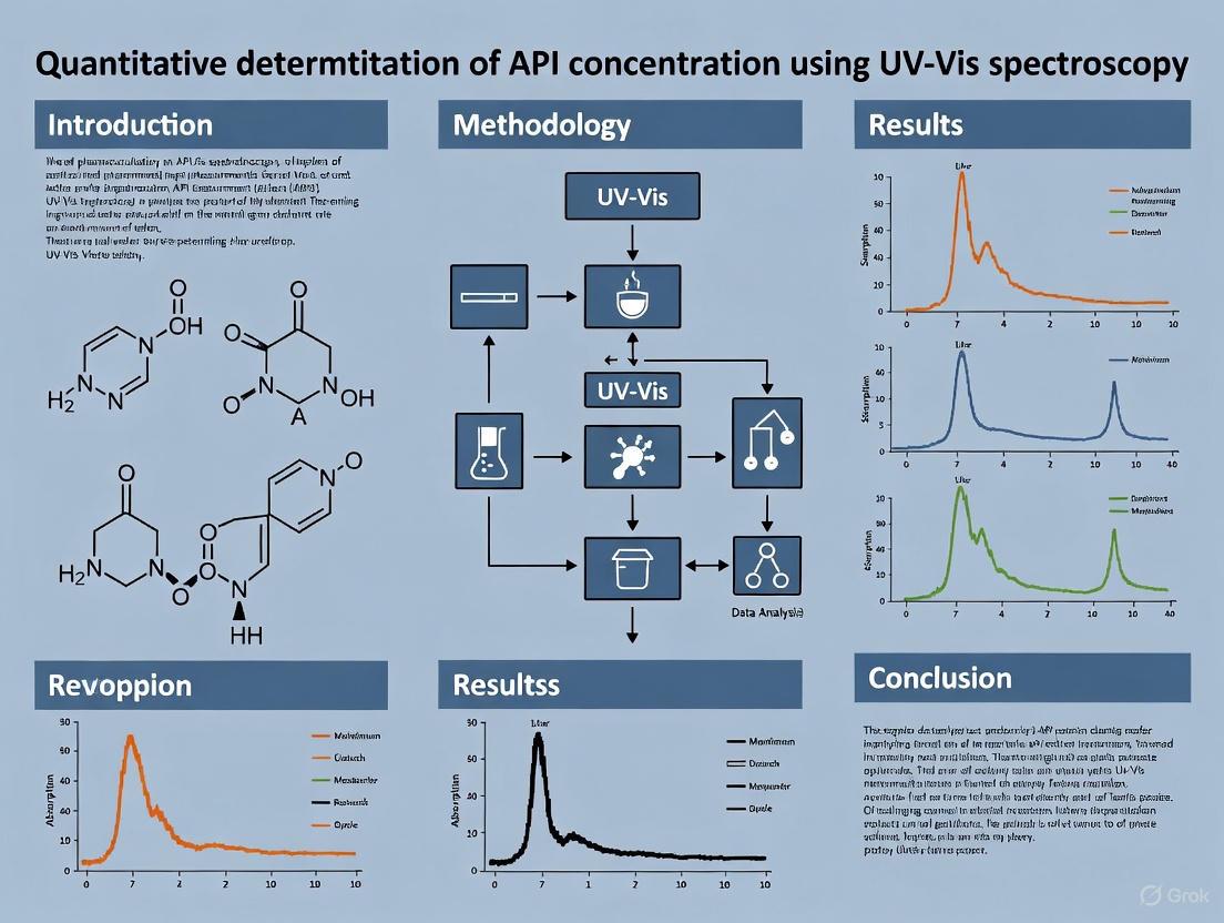
Quantitative Determination of API Concentration by UV-Vis Spectroscopy: A Comprehensive Guide for Pharmaceutical Scientists

Abstract

This article provides a comprehensive examination of UV-Vis spectroscopy for quantifying active pharmaceutical ingredient (API) concentration throughout the drug development lifecycle. It covers fundamental principles based on the Beer-Lambert law, explores diverse methodological approaches including specific assays and advanced chemometric techniques, and addresses common troubleshooting scenarios with practical optimization strategies. The content further examines rigorous validation protocols following ICH guidelines and comparative analysis of quantification methods, incorporating recent advances in Process Analytical Technology (PAT) and real-time monitoring applications. Designed for researchers, scientists, and drug development professionals, this guide bridges theoretical foundations with practical implementation to ensure accurate, reliable API quantification in pharmaceutical products.

UV-Vis Spectroscopy Fundamentals: Principles and Scope for API Analysis

The Beer-Lambert Law (also known as Beer's Law) is a fundamental principle in optical spectroscopy that defines the relationship between the attenuation of light through a substance and the properties of that substance [1]. This law forms the theoretical foundation for the quantitative analysis of active pharmaceutical ingredients (APIs) using ultraviolet-visible (UV-Vis) spectroscopy, enabling researchers to determine analyte concentration through simple absorbance measurements [2].

The law states that the absorbance of light by a solution is directly proportional to the concentration of the absorbing species and the path length of light through the solution [3]. This linear relationship enables pharmaceutical scientists to develop accurate and precise analytical methods for API quantification during various stages of drug development, manufacturing, and quality control [4]. The application of this principle is particularly valuable in pharmaceutical analysis because it provides a rapid, non-destructive means of quantifying drug substances and products while complying with regulatory guidelines such as ICH Q2(R1) [4] [5].

Theoretical Foundations

Mathematical Formulation

The Beer-Lambert Law is mathematically expressed as:

A = εlc

Where:

• A is the absorbance (dimensionless)
• ε is the molar absorptivity or molar extinction coefficient (L·mol⁻¹·cm⁻¹)
• l is the path length of light through the solution (cm)
• c is the concentration of the absorbing species (mol/L) [1] [2] [3]

The absorbance (A) is defined through the relationship between the incident light intensity (I₀) and transmitted light intensity (I):

A = log₁₀(I₀/I) [1] [2]

This logarithmic relationship means that absorbance increases as transmittance decreases. The following table illustrates this inverse relationship between absorbance and transmittance:

Table 1: Relationship Between Absorbance and Transmittance

Absorbance (A)	Transmittance (%)
0	100%
1	10%
2	1%
3	0.1%
4	0.01%
5	0.001%

[1]

Historical Context and Terminology

The principle now known as the Beer-Lambert Law combines the work of three scientists: Pierre Bouguer, Johann Heinrich Lambert, and August Beer [6] [7]. Bouguer and Lambert established the relationship between path length and light attenuation, while Beer demonstrated the proportionality between absorbance and concentration [7]. Modern literature sometimes refers to this combined principle as the Bouguer-Beer-Lambert Law to acknowledge all contributors [6].

The term absorbance has replaced the older term "optical density" (OD), which is now discouraged by IUPAC [1]. While absorbance is technically dimensionless, it is sometimes reported in "absorbance units" (AU), though this practice is redundant and should be avoided [1].

Practical Application to API Quantification

Fundamental Principles in Pharmaceutical Analysis

In pharmaceutical development, UV-Vis spectroscopy leveraging the Beer-Lambert Law serves as a cornerstone technique for API quantification [4] [8]. The linear relationship between absorbance and concentration enables the creation of calibration curves that translate instrumental absorbance readings into precise concentration values for unknown samples [1].

The application of this principle spans multiple critical areas in pharmaceutical analysis:

• Assay of active ingredients: Quantitative measurement of the main therapeutic compound in drug products or raw materials [4]
• Impurity profiling: Detection and characterization of known and unknown impurities [4]
• Dissolution testing: Measurement of the rate and extent of API dissolution from solid dosage forms [4]
• Content uniformity: Assessment of uniform API distribution across multiple dosage units [4]
• Stability testing: Monitoring of API concentration and degradation product formation over time [9]

Experimental Workflow for API Quantification

The following diagram illustrates the logical workflow for API quantification using the Beer-Lambert Law:

Sample Preparation Protocols

Drug Substance (API) Sample Preparation

Proper sample preparation is critical for accurate API quantification [9]. The "dilute and shoot" approach is commonly employed for drug substances:

• Weighing: Accurately weigh 25-50 mg of API reference standard or sample using a five-place analytical balance (±0.1 mg accuracy) [9].
• Transfer: Quantitatively transfer the powder to an appropriately sized Class A volumetric flask using a folded weighing paper or weighing boat to minimize spillage [9].
• Solubilization: Add diluent and dissolve using one of the following methods:
  • Sonication: Use an ultrasonic bath for a specified time determined during method development
  • Shaking: Employ a wrist-action or orbital shaker
  • Vortex mixing: Use a vortex mixer for rapid dissolution [9]
• Dilution: Dilute to volume with the appropriate solvent, ensuring complete dissolution of the API [9].
• Transfer to HPLC vial: Pipette an aliquot (typically 1.5 mL) into an HPLC vial for analysis [9].

Table 2: Key Considerations for Drug Substance Sample Preparation

Parameter	Requirement	Precautions
Weighing Accuracy	±0.1 mg	Use microbalance for samples <20 mg
Diluent Selection	Compatible with API solubility and stability	Avoid solvents causing peak anomalies in HPLC
Solubilization	Complete dissolution verified visually	Prolonged sonication may cause degradation
Hygroscopic APIs	Speedy handling required	Allow refrigerated samples to reach room temperature before opening

[9]

Drug Product Sample Preparation

For drug products such as tablets and capsules, a more elaborate "grind, extract, and filter" approach is typically employed:

• Particle Size Reduction:
  • For tablets: Crush 10-20 units in a porcelain mortar and pestle
  • For capsules: Open and empty contents directly into volumetric flask [9]
• Transfer: Quantitatively transfer all particles to an appropriate volumetric flask [9].
• Extraction: Add diluent and extract using sonication, shaking, or vortex mixing [9].
• Filtration: Filter the extract through a 0.45 μm membrane filter, discarding the first 0.5 mL of filtrate [9].

Advanced Applications and Case Studies

In-line API Concentration Measurement in Nanoparticle Production

UV-Vis spectroscopy based on the Beer-Lambert Law has been successfully implemented as a Process Analytical Technology (PAT) tool in advanced pharmaceutical manufacturing processes. A recent application involves the Controlled Expansion of Supercritical Solutions (CESS) process, a nanoparticle production technology used to enhance the dissolution rate of poorly soluble APIs [10].

In this advanced implementation:

• A custom-made pressure and temperature-rated transmission flow-through cell was designed to interface with the supercritical carbon dioxide (scCO₂) process stream [10].
• In-process calibration was developed to correlate UV-Vis absorption spectra to API concentration in scCO₂ [10].
• The method accounted for density-dependent molar absorption coefficients of the API in scCO₂, requiring calibration for each combination of temperature and pressure [10].
• This PAT tool provided real-time insight into process efficiency and enabled real-time API quantity estimation [10].

Protein and Nucleic Acid Quantification

The Beer-Lambert Law finds extensive application in biopharmaceutical analysis for quantifying proteins, DNA, and RNA [8]. Modern UV-Vis spectrometers can accurately measure biomolecule concentrations using minimal sample volumes (2 μL) across wide dynamic ranges [8].

Table 3: UV-Vis Absorption Characteristics of Key Biomolecules

Biomolecule	Absorption Maximum (nm)	Typical Quantification Range
Proteins	280 nm	0.02 - 200 mg/mL (IgG)
DNA/RNA	260 nm	1.5 - 13,750 ng/μL

[8]

Method Validation and Regulatory Considerations

Analytical Method Validation Parameters

According to ICH Q2(R1) guidelines, analytical methods based on the Beer-Lambert Law must be properly validated to ensure reliability and regulatory compliance [4]. Key validation parameters include:

• Specificity: Ability to measure the API accurately in the presence of potential interferents like excipients, degradation products, or impurities [4].
• Accuracy: Closeness of test results to the true value, typically demonstrated through recovery studies (98-102% recovery for APIs) [4].
• Precision: Degree of repeatability under normal operating conditions, including:
  • Repeatability (same analyst, equipment, short interval)
  • Intermediate precision (different analysts, equipment, days)
  • Reproducibility (across different laboratories) [4]
• Linearity: Ability to obtain results proportional to analyte concentration, typically demonstrated with a minimum of 5 concentration levels and a correlation coefficient (R²) ≥ 0.999 [4].
• Robustness: Method resilience to small, deliberate variations in parameters like flow rate, temperature, or mobile phase composition [4].

The Scientist's Toolkit: Essential Materials for API Quantification

Table 4: Key Research Reagent Solutions and Materials for API Quantification

Item	Function	Application Notes
Class A Volumetric Flasks	Precise volume containment	Critical for accurate dilution and concentration calculations
Five-Place Analytical Balance	Accurate sample weighing (±0.1 mg)	Essential for preparing standard solutions of known concentration
UV-Vis Spectrophotometer	Absorbance measurement	Must be properly calibrated and qualified
Reference Standards	Calibration and method validation	Qualified API reference standard with known purity
HPLC-Vials	Sample containment during analysis	Amber vials required for light-sensitive compounds
Syringe Filters (0.45 μm)	Particulate removal from drug product extracts	Nylon or PTFE membrane; first 0.5 mL discarded
Appropriate Diluents	Solubilization of API	Selected based on API solubility and stability characteristics

[4] [9] [8]

Limitations and Practical Considerations

Fundamental Limitations of the Beer-Lambert Law

While the Beer-Lambert Law provides an excellent foundation for API quantification, several limitations must be considered:

• Chemical Deviations: Occur due to analyte associations, dissociations, or interactions with the solvent at high concentrations [3] [6].
• Instrumental Deviations: Result from the use of polychromatic light, stray light, or improper spectrometer alignment [6].
• Electromagnetic Deviations: Arise from the wave nature of light, including band shifts and intensity changes based on optical conditions [6].
• High Concentration Limitations: The linear relationship fails at higher concentrations due to changes in refractive index and molecular interactions [3] [6].

Troubleshooting Common Issues

The following workflow outlines a systematic approach to troubleshooting Beer-Lambert Law applications in API quantification:

The Beer-Lambert Law remains a cornerstone principle in pharmaceutical analysis, providing a robust foundation for API quantification across drug development, manufacturing, and quality control. Its mathematical simplicity belies its powerful utility in translating simple absorbance measurements into accurate concentration data. When properly implemented with appropriate sample preparation, method validation, and understanding of its limitations, this fundamental law enables scientists to generate reliable, regulatory-compliant data essential for ensuring drug safety and efficacy. As pharmaceutical technologies advance, the integration of Beer-Lambert principles with modern PAT tools continues to expand its applications in innovative manufacturing processes like nanoparticle production, demonstrating the enduring relevance of this fundamental spectroscopic relationship.

Ultraviolet-Visible (UV-Vis) spectroscopy is a foundational analytical technique in pharmaceutical research for the quantitative determination of Active Pharmaceutical Ingredient (API) concentration. The principle underpinning this technique is the measurement of the amount of discrete wavelengths of ultraviolet or visible light (typically 190 nm to 800 nm) that are absorbed by or transmitted through a sample compared to a reference or blank sample [11] [12]. This absorption of light occurs when electrons in a molecule's chromophores are promoted from a ground energy state to a higher energy state, a process known as an electronic transition [12] [13]. The specific wavelength absorbed is characteristic of the molecular structure, while the extent of absorption is directly related to the concentration of the analyte via the Beer-Lambert Law [11] [12].

The Beer-Lambert Law is expressed as: A = εlc Where:

• A is the measured Absorbance (unitless)
• ε is the molar absorptivity (L mol⁻¹ cm⁻¹)
• l is the optical path length of the sample holder (cm)
• c is the concentration of the substance (mol L⁻¹) [11] [12]

This relationship is the cornerstone of API quantification, allowing researchers to construct calibration curves from standards of known concentration to determine the unknown concentration of a drug substance in a sample with high accuracy and precision [12]. The technique is valued for being cost-effective, simple, versatile, and non-destructive, permitting the sample to be used for further analysis if required [12].

Detailed Component Analysis

The accurate application of the Beer-Lambert Law relies on the precise functioning of several key instrumental components. The typical layout of a UV-Vis spectrophotometer involves a light source, a wavelength selector, a sample holder, and a detector.

A stable light source emitting radiation across a wide spectrum is essential. No single lamp covers the entire UV-Vis range optimally, so instruments often use a combination of sources, with an automatic switchover around 300-350 nm where their light emission is comparable [11] [12] [14].

Table 1: Characteristics of Common UV-Vis Light Sources

Light Source	Spectral Range	Principle & Characteristics	Typical Use Case
Deuterium Lamp [11] [14]	190 nm - 400 nm (UV)	Continuous spectrum; good intensity in the UV region; often paired with a halogen lamp.	Primary source for ultraviolet wavelength measurements.
Tungsten/Halogen Lamp [11] [12]	330 nm - 3200 nm (Visible to NIR)	Incandescent filament; robust and stable; intensity decreases in UV region.	Primary source for visible and near-infrared wavelength measurements.
Xenon Lamp [11] [15]	UV and Visible ranges	High-intensity, continuous source; more expensive and less stable than tungsten/halogen lamps.	Sometimes used as a single source for both UV and Vis.

Wavelength Selection: Monochromators and Filters

To analyze a sample at a specific wavelength, the broad spectrum from the light source must be dispersed and selected. The monochromator is the most versatile component for this purpose [11] [12]. Its function is to separate light into a narrow band of wavelengths.

The key elements of a monochromator are:

• Entrance Slit: Controls the width and alignment of the incoming light beam [15].
• Collimating Mirror: Makes the light beam parallel before it strikes the dispersing element [15].
• Diffraction Grating: The core dispersive element. It is a surface with many parallel grooves that diffracts different wavelengths of light at different angles. Rotating the grating selects which narrow band of wavelengths passes through [11] [14]. Holographic gratings with higher groove density (e.g., ≥1200 grooves/mm) generally provide better optical resolution than ruled gratings [11].
• Exit Slit: Allows the selected narrow wavelength band to pass through to the sample [12] [14].

The Spectral Bandwidth (SBW), determined by the width of the slits, is a critical parameter. A narrower SBW provides better spectral resolution, allowing closely spaced absorption peaks to be differentiated. However, it also reduces light throughput, which can increase signal-to-noise. A wider SBW does the opposite, providing more signal but poorer resolution [14]. The SBW should typically be set to 1/10 of the natural width of the sample's absorption peak for optimal results [14].

Filters, including absorption, interference, and bandpass filters, are also used, sometimes in conjunction with monochromators, to further refine wavelength selection or for simpler instruments [11].

Sample Holders

After wavelength selection, the light beam interacts with the sample held in a sample container or cuvette. The choice of cuvette material is critical, as it must be transparent to the wavelengths of interest.

Table 2: Common Sample Holders in UV-Vis Spectroscopy

Cuvette Type	Wavelength Range	Characteristics & Applications
Quartz / Fused Silica [11] [12]	190 nm - 2500 nm (Far UV to NIR)	Transparent across the entire UV-Vis range; essential for UV measurements below ~350 nm.
Glass [11]	~350 nm - 2000 nm (Visible to NIR)	Absorbs most UV light; suitable for measurements in the visible range only.
Plastic [11]	Visible range (varies)	Inexpensive and disposable; generally absorbs UV light and is not suitable for accurate UV work.

The standard path length is 1 cm, but shorter path lengths (e.g., 1 mm) are available for highly concentrated samples to keep absorbance within the instrument's optimal dynamic range (typically Absorbance < 1) [11]. Furthermore, modern cuvette-free systems exist for analyzing very small sample volumes (e.g., 0.5 μL for DNA/RNA analysis) using surface tension to hold the sample [11] [15].

The instrument can be single-beam or double-beam. In a single-beam setup, all light passes through the sample, and the reference measurement is taken separately. In a double-beam setup, the light is split into two paths: one through the sample and one through a reference solvent (blank), allowing for simultaneous measurement and automatic correction for source fluctuations [12] [14].

Detectors

The detector converts the intensity of light transmitted through the sample (I) into an electrical signal proportional to the light's intensity. This signal is then compared to that from the reference beam (I₀) to calculate absorbance [11] [15].

Table 3: Detectors Used in UV-Vis Spectrophotometry

Detector Type	Principle of Operation	Sensitivity & Applications
Photomultiplier Tube (PMT) [11] [14]	Based on the photoelectric effect. Incident photons eject electrons from a photocathode, which are then amplified through a series of dynodes.	Very high sensitivity and low noise; excellent for detecting low light levels. Widely used in high-performance instruments.
Silicon Photodiode [11] [14]	A semiconductor device. Photons with energy greater than the bandgap of silicon create electron-hole pairs, generating a photocurrent.	Fast response, robust, and lower cost than PMTs; slightly less sensitive. Common in many modern spectrophotometers.
Charge-Coupled Device (CCD) [11]	An array of light-sensitive semiconductor elements (pixels) that can capture an entire spectrum simultaneously.	Used in diode-array instruments where the grating is before the sample, allowing multi-wavelength detection.

The following diagram illustrates the logical sequence and configuration of these core components within a standard UV-Vis spectrophotometer.

Application in API Quantification: Protocols and Experimental Design

Detailed Protocol: API Content Uniformity in Tablets

This protocol outlines the use of UV-Vis spectroscopy to assess the concentration and content uniformity of an API in a tablet formulation, a critical quality control step in pharmaceutical development [16] [17].

1. Principle: A representative sample of a powdered tablet is dissolved in a suitable solvent. The absorbance of the resulting solution is measured at the wavelength of maximum absorption (λ_max) for the API. The concentration is determined by interpolating the absorbance value against a pre-established calibration curve, following the Beer-Lambert Law [12].

2. Research Reagent Solutions & Materials: Table 4: Essential Materials for API Quantification

Item	Function / Specification
API Reference Standard	High-purity compound for preparing calibration standards.
Tablet Formulation	Includes the API and excipients (e.g., Microcrystalline Cellulose).
Appropriate Solvent	Must dissolve the API and be transparent at analytical wavelengths (e.g., buffered aqueous solution, methanol).
Volumetric Flasks	For precise preparation of standard and sample solutions.
Quartz Cuvettes	For holding samples during analysis; transparent in UV-Vis range.
Analytical Balance	For accurate weighing of standards and sample powders.
Ultrasonic Bath	To aid in the complete dissolution of the powdered tablet.

3. Procedure:

• Step 1: Preparation of Standard Solutions.
  • Accurately weigh a quantity of the API reference standard.
  • Dissolve and dilute to volume in a volumetric flask to create a primary stock solution of known concentration (e.g., 1000 µg/mL).
  • Perform a serial dilution of the stock solution to prepare at least five standard solutions of different concentrations (e.g., 5, 10, 15, 20, 25 µg/mL) that cover the expected concentration range of the sample.

• Step 2: Preparation of Sample Solution.

  • Accurately weigh and finely powder not less than 20 tablets [16].
  • Transfer an accurately weighed portion of the powder, equivalent to the weight of one tablet, into a volumetric flask.
  • Add a suitable solvent, shake, and use an ultrasonic bath to ensure complete extraction of the API from the powder matrix.
  • Dilute to volume and filter if necessary to obtain a clear solution.

• Step 3: Spectral Measurement and Calibration.

  • Using the solvent as a blank, measure the absorbance of each standard solution at the predetermined λ_max of the API.
  • Plot a graph of absorbance (y-axis) versus concentration (x-axis) for the standard solutions. Perform linear regression to obtain the equation of the calibration curve (y = mx + c) and the correlation coefficient (R²). The plot should be linear.

• Step 4: Sample Analysis and Calculation.

  • Measure the absorbance of the prepared sample solution at the same λ_max.
  • Calculate the concentration of the API in the sample solution using the equation from the calibration curve.
  • The concentration in the original tablet is calculated as follows: API mass (mg/tablet) = [Calculated conc. (µg/mL) × Dilution Factor × Flask Volume (mL)] / [1000 µg/mg × Number of tablets extracted]
  • This process is repeated for multiple tablet samples to determine content uniformity [16].

Advanced Application: Chemometric Analysis for Multicomponent Formulations

A significant challenge in pharmaceutical analysis is the quantification of multiple APIs in a single formulation (Fixed-Dose Combinations) where their absorption spectra overlap. Traditional single-wavelength analysis fails here. The solution is to couple UV-Vis spectroscopy with chemometric models [17].

Protocol Overview:

• Step 1: Experimental Design. A factorial design is used to prepare a large set of synthetic mixtures containing varying, known concentrations of all APIs (e.g., CLZ and DAP for leprosy treatment) and potential excipients [17].
• Step 2: Spectral Acquisition. The full UV-Vis absorption spectrum (e.g., 200-700 nm) is acquired for each mixture, creating a rich dataset.
• Step 3: Model Development. This dataset is processed using multivariate calibration models.
  • Partial Least Squares (PLS) Regression: Correlates the spectral data with the known concentration data to build a predictive model [17].
  • Multivariate Curve Resolution-Alternating Least Squares (MCR-ALS): Decomposes the spectral data matrix to resolve the pure spectra and concentration profiles of each component in the mixture, even in the presence of unknown interferences [17].
• Step 4: Validation and Prediction. The models are validated using test sets and compared against reference methods like High-Performance Liquid Chromatography (HPLC). Once validated, the model can rapidly and accurately predict the concentration of all APIs in an unknown sample based solely on its UV-Vis spectrum [17].

The workflow for this advanced, yet increasingly common, application is detailed below.

Critical Performance Considerations and Limitations

While powerful, several instrumental and experimental factors must be controlled to ensure data accuracy in API quantification.

• Stray Light: This is any light that reaches the detector at wavelengths outside the intended bandwidth. It becomes significant when sample absorbance is very high (low transmittance), causing a deviation from the Beer-Lambert Law and resulting in falsely low absorbance readings [14]. Double-monochromator instruments are designed to minimize this effect.
• Photometric Linearity and Dynamic Range: The range of absorbances over which the instrument's response is linear is crucial for accurate quantification. Measurements should ideally be made where absorbance is below 1, as higher values can lead to non-linearity due to factors like stray light [11] [14].
• Spectral Bandwidth Settings: As discussed, an inappropriate bandwidth can lead to poor resolution or excessive noise, distorting absorption peaks and compromising concentration measurements [14].
• Limitations of the Technique: UV-Vis spectroscopy generally has lower sensitivity and selectivity compared to techniques like fluorescence or HPLC. Its selectivity in complex mixtures can be greatly enhanced by the use of chemometrics, as shown in the protocol above [15] [17]. Furthermore, it provides no structural information on its own, and its accuracy is dependent on the careful preparation of standards and samples.

The quantitative determination of Active Pharmaceutical Ingredient (API) concentration is a cornerstone of pharmaceutical development and quality control. Among the various analytical techniques available, ultraviolet-visible (UV-Vis) spectroscopy stands out for its reliability, ease of use, and broad applicability [11]. The technique operates on the principle that molecules absorb light in the UV-Vis range when electrons are promoted to higher energy states, with the amount of absorption being quantitatively related to the concentration of the absorbing species [18]. The successful application of this technique for API quantification hinges on the precise understanding and control of three critical parameters: molar absorptivity, path length, and optimal wavelength selection. These parameters are mathematically interconnected through the Beer-Lambert law, which forms the theoretical foundation for all quantitative UV-Vis analyses [19] [11]. This application note provides detailed protocols and structured data to guide researchers and drug development professionals in optimizing these parameters for robust and reliable API quantification.

Theoretical Foundations

The Beer-Lambert Law

The fundamental principle governing quantitative UV-Vis spectroscopy is the Beer-Lambert Law. It states that the absorbance (A) of light by a solution is directly proportional to the concentration (c) of the absorbing species and the path length (l) of the light through the solution [19] [11]. The law is expressed mathematically as:

A = ε * l * c

Where:

• A is the measured absorbance (no units) [11].
• ε is the molar absorptivity (or molar absorption coefficient), with typical units of L·mol⁻¹·cm⁻¹ [20].
• l is the path length, the distance the light travels through the sample, usually measured in centimeters (cm) [21].
• c is the concentration of the absorbing substance, typically in mol·L⁻¹ [19].

This linear relationship holds true for monochromatic light and dilute solutions, providing the basis for determining the concentration of an unknown sample by measuring its absorbance [19].

Parameter Interdependence and Regulatory Context

The three parameters are deeply intertwined. The sensitivity of a method is largely determined by the molar absorptivity of the API at the chosen wavelength [18]. This sensitivity, in turn, dictates the required path length to achieve an absorbance signal within the ideal dynamic range of the instrument (typically 0.5 to 1.5 AU) for accurate quantitation [21] [11]. For instance, an API with low molar absorptivity may require a longer path length to produce a measurable absorbance signal. The principles of Analytical Quality by Design (AQbD) are now being explored to build robustness into analytical procedures, emphasizing predefined performance requirements outlined in an Analytical Target Profile (ATP) [22]. This systematic, risk-based approach is particularly valuable for in-line Process Analytical Technology (PAT) applications, such as monitoring API concentration during Hot Melt Extrusion (HME), to enable Real Time Release Testing (RTRT) [22].

Critical Parameter Analysis

Molar Absorptivity

Molar absorptivity (ε) is an intrinsic property of a molecule that indicates how strongly it absorbs light at a specific wavelength [20]. Its value is influenced by the electronic structure of the molecule, particularly the presence of light-absorbing groups known as chromophores, and the extent of conjugation in the system [18].

• Significance: A higher molar absorptivity allows for the detection of lower concentrations of an analyte with greater sensitivity [18]. It is a constant for a given substance under defined conditions (solvent, pH, temperature) [20].
• Terminology Clarification: The term "molar absorptivity" is preferred over obsolete terms like "extinction coefficient" [20]. The use of "extinction coefficient" is discouraged, as "extinction" properly refers to the combined effects of absorption, scattering, and luminescence [20].

Table 1: Molar Absorptivity Values for Common Chromophores

Chromophore / Compound	Example λmax (nm)	Example Molar Absorptivity (ε, L·mol⁻¹·cm⁻¹)	Structural Feature
Simple C=C Bond	~171	~10,000	Isolated double bond [18]
Carbonyl (C=O)	180, 290	10000, 15	Aldehydes/Ketones; low ε for n→π* transition [19]
Conjugated Diene (Buta-1,3-diene)	~217	~20,000	Two conjugated double bonds [18]
Conjugated Triene	~250+	~40,000+	Three conjugated double bonds [18]
Piroxicam (in Kollidon VA64)	N/A	Method Validated	API in polymer carrier for HME [22]

Path Length

Path length is the distance the light beam traverses through the sample solution [21]. According to the Beer-Lambert law, absorbance is directly proportional to path length.

• Selection Criteria: The path length is selected to ensure that absorbance values for the concentrations of interest fall within the instrument's optimal dynamic range (ideally 0.5 to 1.5 AU) [21] [11]. For a highly concentrated sample, a short path length is used to avoid exceeding the detectable absorbance limit (>2 AU). Conversely, for a dilute sample, a longer path length is used to enhance the signal [21] [11].
• Standard Sizes and Applications: Common path lengths for cuvettes are 1 cm, while flow cells for HPLC-UV detectors are typically 10 mm with volumes in the microliter range [11] [23]. For specialized applications like protein and DNA analysis, fixed pathlength microcuvettes as short as 0.1 mm are used to handle high concentrations without dilution [8].

Table 2: Common Path Lengths and Their Typical Applications

Path Length	Typical Application Context	Rationale
0.1 mm	Microvolume analysis of proteins/DNA (e.g., Lunatic/Stunner systems) [8]	Prevents dilution of high-concentration samples; wide dynamic range.
1 mm	Small volume or high concentration samples in cuvettes [11]	Reduces absorbance for concentrated analytes.
10 mm (1 cm)	Standard cuvette-based spectrometry; HPLC-UV flow cells [19] [23]	Default configuration for a wide range of concentrations.
20 - 100 mm	Long-path cells for trace analysis of very dilute samples [21]	Increases absorbance signal for low-concentration analytes.

Optimal Wavelength Selection

Selecting the appropriate wavelength is critical for achieving maximum sensitivity and minimizing interference.

• Lambda-max (λmax): This is the wavelength at which a substance has its strongest absorption [18] [23]. Measuring absorbance at λmax provides the highest sensitivity and is generally preferred for quantitation because the slope of the calibration curve is steepest here, reducing relative error [19].
• Spectral Characteristics: The choice of wavelength may also be influenced by the need to avoid interference from other absorbing species in the sample (e.g., excipients, solvents) [11]. In such cases, a secondary, less sensitive wavelength with less interference might be selected.
• Validation: For methods used in regulatory testing, the maximum absorbance wavelength (λmax) for the API must be confirmed experimentally and the method validated per ICH guidelines [22] [23].

Diagram 1: Workflow for UV-Vis Method Development for API Quantification. The workflow outlines the critical steps, highlighting key decision points (red diamond) and essential parameters (yellow rectangles) to establish a validated method.

Experimental Protocols

Protocol 1: Determination of Molar Absorptivity

This protocol outlines the steps to determine the molar absorptivity (ε) of a pure API standard.

Research Reagent Solutions & Materials: Table 3: Essential Materials for Molar Absorptivity Determination

Item	Function / Specification
High-Purity API Standard	The analyte of interest, of known purity and identity.
Appropriate Solvent	Spectroscopic grade, transparent in the spectral region of interest (e.g., HPLC grade methanol) [11].
Volumetric Flasks	For precise preparation of standard solutions (e.g., Class A).
UV-Vis Spectrophotometer	Instrument capable of scanning UV-Vis spectrum.
Cuvettes	With a known, fixed path length (e.g., 1 cm quartz for UV) [11].
Analytical Balance	For accurate weighing of the API standard.

Procedure:

• Stock Solution Preparation: Accurately weigh a known mass of the pure API standard. Dissolve and dilute it with the chosen solvent in a volumetric flask to prepare a stock solution of known concentration (e.g., 1 x 10⁻³ M).
• Dilution Series: Prepare a series of at least 5 standard solutions by diluting the stock solution to different concentrations (e.g., 2 x 10⁻⁵ M, 4 x 10⁻⁵ M, 6 x 10⁻⁵ M, 8 x 10⁻⁵ M, 1 x 10⁻⁴ M). Ensure all concentrations fall within the linear range of the Beer-Lambert law (Absorbance < ~1.5).
• Blank Measurement: Fill a cuvette with the pure solvent and place it in the spectrophotometer. Acquire a spectrum or set the absorbance to zero at the desired wavelength(s). This is your reference or blank [11].
• Sample Measurement: Replace the blank with each standard solution and measure the absorbance value at the previously identified λmax of the API.
• Data Analysis: Plot a graph of the measured absorbance (y-axis) against the corresponding concentration (x-axis) for each standard. Perform linear regression analysis. The slope of the resulting calibration curve is equal to (ε * l). Since the path length (l) is known (e.g., 1 cm), the molar absorptivity (ε) can be calculated as: ε = Slope / l [19].

Protocol 2: Validation of an In-line API Quantification Method using AQbD

This protocol is adapted from a study on monitoring piroxicam in Kollidon VA64 during Hot Melt Extrusion (HME) and exemplifies a modern, risk-based approach [22].

Research Reagent Solutions & Materials:

• API (e.g., Piroxicam) and polymer carrier (e.g., Kollidon VA64).
• Twin-screw hot melt extruder.
• In-line UV-Vis spectrophotometer with high-temperature transmission probes.
• V-cone blender for powder mixing.

Procedure:

• Define the Analytical Target Profile (ATP): The ATP states that the method must predict the API concentration with defined accuracy and precision, for example, with 95% β-expectation tolerance limits within ±5% acceptance limits [22].
• Risk Assessment: Perform a Failure Mode and Effect Analysis (FMEA) to identify risks to the analytical procedure. Critical Analytical Attributes (CAAs) may include colour parameters (L, b) linked to the ability to measure API and transmittance [22].
• System Setup & Calibration: Install the UV-Vis probes in the extruder die in a transmission configuration. Collect a reference transmittance signal with an empty die at process temperature. Develop a predictive model based on UV-Vis absorbance spectra collected during extrusion of calibration samples with known API concentrations [22].
• Method Validation via Accuracy Profile: The method's validity is based on the accuracy profile strategy, which uses β-expectation tolerance intervals calculated from validation data. The method is considered valid if these tolerance limits lie within the pre-defined acceptance limits (±5%) for all concentration levels studied [22]. This approach is a robust alternative to traditional one-off validation and aligns with ICH Q2(R1) criteria and its revisions [22].

The Scientist's Toolkit

A successful UV-Vis spectroscopy method for API quantification relies on several key components and reagents.

Table 4: Key Research Reagent Solutions and Essential Materials

Item / Reagent	Function / Critical Role in API Quantification
Spectroscopic Grade Solvents	High-purity solvents (e.g., methanol, acetonitrile, water) are essential to minimize background absorbance and interference in the UV range [11].
API Standard	A high-purity, well-characterized reference standard of the Active Pharmaceutical Ingredient, used for calibration and method validation.
Quartz Cuvettes	Required for UV range analysis as quartz is transparent to UV light; standard path length is 1 cm [11].
UV-Vis Spectrophotometer	The core instrument, comprising a light source (D₂ lamp for UV), wavelength selector (monochromator or DAD), and detector (e.g., photomultiplier tube) [11] [23].
HPLC-UV/VIS System	For separation-based quantification, consisting of a pump, injector, column, and UV detector (VWD or DAD) with a low-volume flow cell [23].
Process Analytical Technology (PAT) Tool	In-line UV-Vis probes for real-time monitoring of API concentration in manufacturing processes like Hot Melt Extrusion (HME) [22].
Volumetric Glassware	Precise flasks and pipettes for accurate preparation of standard and sample solutions, critical for generating reliable calibration curves.

Diagram 2: Interrelationship of Critical Parameters in UV-Vis Quantification. This diagram illustrates how the three core parameters of the Beer-Lambert law interact, showing that molar absorptivity is an intrinsic molecular property, while path length and wavelength are selected by the experimenter to optimize sensitivity, dynamic range, and specificity.

The accurate quantitative determination of API concentration by UV-Vis spectroscopy is fundamentally dependent on a rigorous understanding and optimization of molar absorptivity, path length, and optimal wavelength selection. Molar absorptivity is an intrinsic property dictating the method's potential sensitivity, while path length is a practical tool to adjust the absorbance signal into the instrument's optimal working range. The selection of the analytical wavelength, preferably at λmax, ensures maximum sensitivity and minimal interference. By following a systematic, quality-by-design approach—from defining the ATP to method validation via accuracy profiles—researchers can develop robust analytical procedures suitable for both laboratory analysis and in-line process monitoring, thereby ensuring product quality and safety throughout the drug development lifecycle.

In the quantitative determination of Active Pharmaceutical Ingredient (API) concentration by UV-Vis spectroscopy, the method of sample presentation is a critical foundational step that directly influences data accuracy, reproducibility, and regulatory compliance. The interface between your sample and the spectrophotometer's light beam must be meticulously controlled to ensure that measurements reliably reflect the sample's true properties rather than artifacts of the holding apparatus. Errors in selection can lead to inaccurate concentration values, potentially compromising drug quality and safety assessments. This guide details the practical considerations for selecting and using cuvettes, flow cells, and solid sampling accessories, with a specific focus on applications in pharmaceutical development.

Cuvette Selection: Materials and Geometries

The cuvette is the most common accessory for liquid sample analysis. Its material dictates the usable wavelength range and chemical compatibility, while its geometry determines pathlength and sample volume.

Material Selection for Pharmaceutical Applications

The choice of cuvette material is paramount for ensuring accurate UV-Vis analysis, as it sets the fundamental limits for wavelength transmission, chemical resistance, and signal-to-noise ratio [24] [25] [26].

Table 1: Cuvette Material Properties and Selection Guide

Material	Transmission Range	Best Use Cases in API Analysis	Chemical Resistance	Cost & Lifespan
UV-Grade Quartz (Fused Silica)	~190 – 2500 nm [24] [25] [26]	API quantification in UV range (<300 nm), high-precision assays, methods using aggressive solvents [24] [25].	Excellent against most acids, bases, and organic solvents. Not compatible with HF [24].	Higher upfront cost; reusable for years with proper care [24].
Optical Glass	~320 – 2500 nm [25] [26]	Visible-range colorimetric assays for dissolution testing or excipient compatibility [25].	Good, but degrades with long-term exposure to strong acids/bases [24].	Moderate cost; reusable for months to years [24].
Plastic (PS/PMMA)	~380 – 780 nm (Visible) [24] [26]	Rapid, disposable checks in visible light (e.g., Bradford protein assay); teaching labs [24] [26].	Poor; attacked by acetone, ethanol, DMSO, and other organics [24].	Lowest cost; designed for single use [24].
UV-Transparent Plastic	~220 – 900 nm [26]	Disposable alternative for UV quantification of APIs when quartz is unavailable; pilot studies [26].	Limited chemical resistance; not suitable for long-term storage [26].	Low cost; disposable [26].

For API quantification, where measurements often occur at UV wavelengths (e.g., 260 nm for nucleic acids, 280 nm for proteins, or other specific API maxima), quartz cuvettes are the unequivocal standard [24] [25]. Their superior transmission in the deep UV and excellent chemical durability make them indispensable for development and quality control labs. Using glass or plastic for UV measurements will block the signal and lead to flawed data [24].

Path Length and Volume Considerations

The optical path length is a direct variable in the Beer-Lambert law (A = εbc). Selecting the correct path length allows for the optimization of the absorbance signal for a given sample concentration [25].

Table 2: Guide to Cuvette Path Length and Volume Selection

Path Length	Sensitivity Gain (vs. 1 mm)	Ideal Sample Volume Type	Pharmaceutical Application Example
1 mm	Baseline	Micro-volume (≈ 50 - 350 µL) [26]	Highly concentrated API solutions to avoid signal saturation [25].
10 mm (Standard)	~10x [25]	Standard volume (≈ 3.0 - 3.5 mL) [24] [26]	Routine quantification of APIs in standard solutions; general QC testing [24].
20 - 50 mm	20x - 50x [25]	Large volume (> 3.5 mL) [26]	Trace analysis of impurities or degradation products in low-concentration solutions [25].

For precious or limited API samples, semi-micro (volume ~1.0 mL) or micro (volume ~50 µL) cuvettes that maintain a 10 mm path length through a reduced cross-section are available [24] [26]. It is critical to ensure the cuvette's center height (typically 8.5 mm, 12.5 mm, or 15 mm) matches the beam height of your spectrophotometer [25].

Advanced and Specialized Sampling Methods

Beyond standard cuvettes, several specialized accessories address unique challenges in process analysis and solid sample characterization.

Flow Cells for Process Analytical Technology (PAT)

Flow cells are integral to Process Analytical Technology (PAT) initiatives, enabling real-time, in-line monitoring of API concentration during bioprocessing or manufacturing. A novel approach involves a disposable, gamma-sterilized flow cell made from biocompatible polymers like Polyamide (PA) or PMMA, which is clamped into a reusable holder within a bypass system. This setup allows for continuous UV-Vis spectroscopy and fluorescence monitoring of critical process parameters without risk of contamination [27].

Another advanced flow cell design enhances sensitivity in droplet-based microfluidic systems. This method involves removing the carrier oil via a PTFE membrane post-reaction, converting droplets into a single-phase stream. The aqueous sample is then measured in a 3D-printed U-shape flow cell with an extended path length (e.g., 5-20 mm), overcoming the sensitivity limitations of traditional short-pathlength microfluidic channels and enabling precise quantification of trace analytes [28].

Accessories for Solid Sample Analysis

Many commercial spectrophotometers are designed for liquids, creating a significant challenge for analyzing solid dosage forms like tablets or films. While specialized solid-sample accessories exist, they can be expensive or unavailable for many instruments [29].

A modern, low-cost solution is the use of 3D-printed cuvette adapters. Two versions have been demonstrated for use in standard UV-Vis and Circular Dichroism (CD) spectrometers [29]:

• Stationary Cuvette: Holds a solid sample (e.g., a 10x10x1 mm film) in a fixed orientation using an internal washer-aperture system. Ideal for standard transmission measurements.
• Rotating Cuvette: Incorporates a bearing-and-washer aperture system, allowing for precise rotation of the solid sample about the beam axis. This is essential for techniques like CD spectroscopy or for measuring the polarization dependence of anisotropic materials [29].

These adapters, fabricatable for less than $1, provide a flexible and accessible means to characterize the optical properties of solid pharmaceutical materials, such as polymer films or composite dosage forms [29].

Experimental Protocols for API Analysis

Protocol 1: Standard API Quantification using a Quartz Cuvette

This protocol outlines the steps for the precise quantification of API concentration in a solution using a standard quartz cuvette.

Diagram: Workflow for Standard API Quantification

Materials & Reagents:

• Spectrophotometer: UV-Vis spectrophotometer calibrated for wavelength and photometric accuracy [30].
• Cuvette: High-quality quartz cuvette, 10 mm path length (or as appropriate).
• Solvents & Solutions: Appropriate high-purity solvent (e.g., water, buffer, alcohol); blank solution (solvent only); API standard solutions of known concentration; unknown API sample solution.

Procedure:

• Cuvette Cleaning: Thoroughly clean the quartz cuvette with a compatible, high-purity solvent. Use lint-free swabs (e.g., microfiber) to avoid scratching the optical surfaces. Avoid ultrasonic baths for coated cells [25].
• Blank Measurement: Rinse the cuvette with the blank solution. Fill it with the blank, ensuring no air bubbles are trapped. Wipe the optical windows with a lint-free tissue. Place it in the spectrophotometer holder and perform a blank measurement to set the 0.000 A baseline [25].
• Sample Measurement: Empty the cuvette. Rinse it twice with a small amount of your API sample solution to prevent dilution. Fill the cuvette with the sample, wipe the windows, and place it in the holder. Measure the absorbance at the predetermined maximum absorption wavelength (λmax) of the API.
• Data Analysis: Calculate the API concentration using the Beer-Lambert law (A = εbc). The molar absorptivity (ε) can be determined from a calibration curve constructed using standard solutions of known concentration.

Protocol 2: Solid Dosage Form Analysis using a 3D-Printed Adapter

This protocol enables the analysis of solid samples, such as polymer films containing APIs, in an instrument designed for liquids.

Diagram: Workflow for Solid Sample Analysis

Materials & Reagents:

• 3D Printer & Resin: SLA or FDM 3D printer with appropriate resin/filament [29].
• Adapter Components: 3D printed cuvette body, washers, bearings (for rotating version), copper tape [29].
• Solid Sample: e.g., a thin film of aligned carbon nanotubes or a polymer film of dimensions ~10x10x1 mm [29].

Procedure:

• Adapter Fabrication: Design and 3D print the solid sample adapter (stationary or rotating) using CAD software (e.g., SolidWorks) and slicing software (e.g., Chitubox for SLA). For the rotating version, assemble the bearing-and-washer aperture system [29].
• Post-Processing: For SLA-printed parts, remove supports, clean in a bath sonicator to remove excess resin, and UV-cure. Apply copper tape to both sides of the cuvette body to prevent light transmission through the plastic itself [29].
• Sample Loading: Insert the solid sample (e.g., a film) into the designated slot or pocket of the adapter.
• Measurement: Place the entire adapter into the spectrophotometer's standard cuvette holder. For isotropic samples, perform a single transmission or absorbance measurement. For anisotropic samples using the rotating cuvette, take measurements at multiple azimuthal orientations (e.g., every 45 degrees) to characterize alignment or polarization effects [29].

The Scientist's Toolkit

Table 3: Essential Research Reagent Solutions and Materials

Item	Function/Explanation	Example Use Case
Quartz Cuvettes (4-window)	Allows light entry and detection from multiple angles; essential for fluorescence assays due to low autofluorescence [24].	Fluorescence-based impurity detection or protein binding studies.
Black-Walled Quartz Cuvettes	Absorbs stray light, significantly improving signal-to-noise ratio for dilute samples and fluorescence measurements [31].	High-sensitivity measurement of low-concentration API degradation products.
Peltier Thermostatted Cuvette Holder	Provides precise temperature control (e.g., 0°C to 110°C) for the cuvette, enabling kinetic studies of API stability or degradation [30].	Studying API degradation kinetics at elevated temperatures.
NIST-Traceable Stray Light Standards	Verification standards (e.g., Potassium Dichromate) used to qualify instrument performance, ensuring photometric accuracy and compliance [30].	Routine performance qualification (PQ) of the UV-Vis spectrophotometer for GMP/GLP environments.
Fiber Optic Probe Coupler	Enables the use of fiber optic probes for remote sampling, allowing measurement directly in containers without transferring the sample to a cuvette [30].	In-line monitoring of API concentration in a reactor vessel during synthesis.

The accurate quantification of API concentration by UV-Vis spectroscopy is heavily dependent on appropriate sample presentation. For most liquid-based assays, the selection of a high-purity quartz cuvette with an optimized path length is non-negotiable for reliable UV-range data. For specialized applications, flow cells enable real-time process monitoring, while innovative, low-cost 3D-printed adapters unlock the analysis of solid dosage forms on standard instruments. By understanding and implementing these methods, researchers and drug development professionals can ensure that their analytical data meets the high standards of accuracy and precision required in the pharmaceutical industry.

Strengths and Limitations of UV-Vis for Pharmaceutical Analysis

Ultraviolet-Visible (UV-Vis) spectroscopy serves as a cornerstone analytical technique in pharmaceutical development and quality control. This application note details the fundamental principles, operational strengths, and inherent limitations of UV-Vis spectroscopy, with a specific focus on the quantitative determination of Active Pharmaceutical Ingredient (API) concentration. Framed within the context of a broader research thesis on API quantification, this document provides detailed experimental protocols and data analysis techniques to guide researchers, scientists, and drug development professionals in implementing robust, reliable analytical methods. The discussion is supported by structured data, experimental workflows, and reagent specifications to facilitate practical application in pharmaceutical analysis.

UV-Vis spectroscopy is an analytical technique that measures the amount of discrete wavelengths of ultraviolet or visible light absorbed by or transmitted through a sample in comparison to a reference or blank sample [11]. This property is directly influenced by sample composition, providing critical information about the identity and concentration of analytes. In pharmaceutical sciences, the technique is indispensable because most drug entities possess chromophores that absorb light in the range of 190–800 nm [32]. The foundational principle governing quantitative analysis is the Beer-Lambert Law (A = εlc), which states that absorbance (A) is proportional to the concentration (c) of the absorbing species, the path length (l) of the sample, and its molar absorptivity (ε) [11]. This relationship enables the precise quantification of APIs throughout drug development, manufacturing, and quality assurance processes.

Fundamental Principles and Instrumentation

Core Components of a UV-Vis Spectrophotometer

A UV-Vis spectrophotometer consists of several key components that work in concert to generate reliable absorbance data [11]:

• Light Source: Provides a steady source emitting light across a wide range of wavelengths. Instruments often employ two lamps: a deuterium lamp for UV light and a tungsten or halogen lamp for visible light [11].
• Wavelength Selector: Typically a monochromator containing a diffraction grating that separates light into a narrow band of wavelengths. This component selects specific wavelengths for sample examination from the broad spectrum emitted by the source [11].
• Sample Holder: Contains the sample for analysis. For UV studies, quartz cuvettes are essential as they are transparent to most UV light, unlike plastic or glass which can absorb UV wavelengths [11].
• Detector: Converts light that has passed through the sample into an electronic signal. Common detectors include photomultiplier tubes (PMTs), photodiodes, and charge-coupled devices (CCDs) [11].

Measurement Principles

When a molecule absorbs UV or visible light, electrons are promoted to higher energy states. The specific amount of energy required for this transition varies depending on the molecular structure and bonding environment of the substance [11]. The resulting absorption spectrum, a plot of absorbance versus wavelength, serves as a unique fingerprint for compound identification and quantification. For quantitative work, absorbance readings should ideally fall within the range of 0.1–1.0 absorbance units (AU) to ensure accuracy, as values outside this range may exceed the instrument's linear dynamic range [11] [33].

Strengths of UV-Vis Spectroscopy in Pharmaceutical Analysis

UV-Vis spectroscopy offers numerous advantages that make it particularly suitable for pharmaceutical analysis, especially in the quantitative determination of API concentration.

Table 1: Key Strengths of UV-Vis Spectroscopy in Pharmaceutical Analysis

Strength	Description	Pharmaceutical Application
Rapid Analysis	Fast data acquisition with integration times in the millisecond range [22].	Enables high-throughput screening and real-time process monitoring during manufacturing.
High Sensitivity	Capable of detecting low concentrations of analytes with appropriate pathlength selection.	Quantification of potent low-dose APIs and detection of trace impurities [33].
Simplicity and Ease of Use	Straightforward instrumentation and data interpretation compared to other techniques [33].	Reduces training requirements and facilitates method implementation in QC laboratories.
Non-Destructive Nature	Samples typically remain unaltered after analysis and can be recovered for further testing [33].	Preserves valuable drug substance during development and allows for additional characterization.
Quantitative Accuracy	When properly validated, provides highly accurate concentration data with precision often within 1-2% [8].	Essential for content uniformity testing, potency determination, and batch release [33].
Cost-Effectiveness	Lower instrument acquisition and maintenance costs compared to techniques like HPLC or NMR [33].	Increases accessibility for laboratories with budget constraints and reduces overall testing costs.
Versatility	Applicable to various sample types (solutions, solids) and compatible with multiple accessory configurations.	Supports diverse applications from raw material identification to dissolution testing [32] [34].

Beyond the strengths summarized in Table 1, modern implementations of UV-Vis spectroscopy offer enhanced capabilities through technological innovations. Variable pathlength technology eliminates the need for sample dilution, thereby reducing analyst-related errors and significantly shortening processing times from hours to minutes [35]. This approach, known as slope spectroscopy, uses the relationship A/l = αc (where l is pathlength) to determine concentration directly from the slope of absorbance versus pathlength, making it particularly valuable for analyzing highly concentrated protein solutions up to 300 mg/mL without dilution [35].

Limitations and Considerations

Despite its numerous strengths, UV-Vis spectroscopy presents several limitations that researchers must address during method development and validation.

Table 2: Key Limitations of UV-Vis Spectroscopy in Pharmaceutical Analysis

Limitation	Description	Mitigation Strategy
Chromophore Requirement	Compounds must contain a chromophore that absorbs UV or visible light.	For analytes without chromophores, consider derivatization or alternative techniques like ELSD or CAD [34].
Spectral Interference	Excipients, impurities, or solvents with overlapping absorbances can interfere with API quantification.	Implement background correction, select alternative wavelengths, or employ spectral deconvolution algorithms [22].
Limited Specificity	Provides limited structural information compared to IR or NMR spectroscopy.	For identity confirmation, combine with orthogonal techniques or use hyphenated approaches like LC-UV [33].
Matrix Effects	Complex formulations can cause light scattering or absorption shifts.	Implement rigorous sample preparation, matrix-matched calibration standards, and standard addition methods.
Dilution Requirements	Highly concentrated samples often require dilution to fall within the linear range of the instrument.	Use variable pathlength technology to minimize or eliminate dilution steps and associated errors [35].
Solvent Restrictions	Solvents must be transparent in the spectral region of interest for the analyte.	Select appropriate solvents (e.g., acetonitrile, water, high-purity alcohols) that do not interfere with analysis [11].
Pathlength Precision	Accurate concentration measurements require precise, known pathlengths.	Use high-quality cuvettes with certified pathlengths or instruments with fixed, validated pathlengths [8].

A particularly critical consideration is the linear dynamic range of the instrument. An absorbance of 1 corresponds to 90% of the incoming light being absorbed, with only 10% transmitted to the detector [11]. At high absorbances (typically >1-2 AU), instruments may struggle to quantify small amounts of light reliably, leading to non-linearity and inaccurate results [11]. Solutions include sample dilution or reduction of the effective pathlength, with modern micro-volume instruments employing fixed pathlengths as small as 0.1 mm to extend the measurable concentration range without dilution [8].

Experimental Protocols for API Quantification

Standard Protocol for API Concentration Determination in Simple Formulations

This protocol describes the quantitative determination of API concentration in a simple solution using a UV-Vis spectrophotometer, suitable for drug substance quantification or simple solution-based formulations.

UV-Vis API Quantification Workflow

Materials and Equipment:

• UV-Vis spectrophotometer with appropriate cuvettes
• Analytical balance
• Volumetric flasks
• Micropipettes
• Reference standard of the API
• Appropriate solvent

Procedure:

• Preparation of Standard Solutions:
  • Accurately weigh 10-100 mg of API reference standard and transfer to a volumetric flask.
  • Dissolve and dilute to volume with appropriate solvent to create a stock solution.
  • Prepare a series of standard solutions covering the expected concentration range (e.g., 5-50 μg/mL) by serial dilution.

• Instrument Preparation:

  • Turn on the spectrophotometer and allow it to warm up for at least 30 minutes.
  • Set the detection wavelength to the λmax of the API (previously determined by scanning).
  • Fill a cuvette with solvent blank and place it in the sample holder.

• System Suitability and Calibration:

  • Measure the absorbance of the blank solution and use it to zero the instrument.
  • Measure the absorbance of each standard solution in triplicate.
  • Construct a calibration curve by plotting average absorbance versus concentration.
  • Determine the correlation coefficient (R²), which should be ≥0.995 for acceptable linearity.

• Sample Analysis:

  • Prepare the sample solution at an appropriate dilution to fall within the calibration range.
  • Measure the absorbance of the sample solution in triplicate.
  • Calculate the API concentration using the linear regression equation from the calibration curve.

• Method Validation:

  • Assess accuracy through recovery studies (typically 98-102%).
  • Determine precision as relative standard deviation (RSD ≤2%).
  • Establish the limit of detection (LOD) and limit of quantification (LOQ).

Advanced Protocol: In-line API Monitoring During Hot Melt Extrusion

This protocol describes the implementation of in-line UV-Vis spectroscopy as a Process Analytical Technology (PAT) tool for real-time monitoring of API concentration during hot melt extrusion (HME), based on the principles of Analytical Quality by Design (AQbD) [22].

Materials and Equipment:

• Twin-screw hot melt extruder
• In-line UV-Vis spectrophotometer with transmission probes
• Optical fiber cables
• API (e.g., piroxicam) and polymer carrier (e.g., Kollidon VA64)

Procedure:

• Analytical Target Profile (ATP) Definition:
  • Define the ATP for the analytical procedure, specifying requirements for accuracy (±5%), precision, and range (e.g., 10-20% w/w API) [22].

• Instrument Setup and Configuration:

  • Install UV-Vis transmission probes into the extruder die.
  • Collect reference transmittance signal with empty die at process temperature (e.g., 140°C).
  • Configure data collection parameters: wavelength range 230-816 nm, resolution 1 nm, frequency 0.5 Hz [22].

• Multivariate Model Development:

  • Prepare calibration standards covering the expected API concentration range.
  • Collect UV-Vis transmittance spectra under various process conditions.
  • Develop predictive models correlating spectral data with known API concentrations.
  • Include colour parameters (L, a, b*) from CIELAB colour space as Critical Analytical Attributes [22].

• Real-Time Monitoring and Validation:

  • Monitor API concentration continuously during HME process.
  • Validate method using accuracy profile strategy with β-expectation tolerance limits (±5%) [22].
  • Test robustness by evaluating effects of process parameters (screw speed, feed rate).

• Data Analysis and Reporting:

  • Apply the predictive model to convert real-time spectral data to API concentration.
  • Generate continuous concentration profiles and trend analysis.
  • Implement statistical process control for automated out-of-specification detection.

Essential Research Reagent Solutions

Successful implementation of UV-Vis methods for pharmaceutical analysis requires specific reagents and materials to ensure accurate and reproducible results.

Table 3: Essential Research Reagents and Materials for UV-Vis Pharmaceutical Analysis

Reagent/Material	Function	Application Notes
High-Purity Solvents	Dissolve analyte without interfering absorbances in spectral region of interest.	Use HPLC-grade solvents; check UV cutoff before use [33].
API Reference Standards	Provide known purity material for calibration curve construction.	Use certified reference materials with documented purity and storage history.
Quartz Cuvettes	Hold samples for analysis with minimal UV light absorption.	Required for UV range; use matched pairs for high-accuracy work [11].
Buffer Components	Maintain constant pH to ensure consistent ionization state of analyte.	Select buffers with low UV absorbance (e.g., phosphate, borate).
Degassing Equipment	Remove dissolved gases that can form bubbles and cause light scattering.	Particularly important for high-precision measurements and automated systems.
Spectrophotometric Cells	Enable variable pathlength measurements without dilution.	Used in systems like Solo VPE for concentrated protein solutions [35].

Regulatory Considerations and Method Validation

The implementation of UV-Vis spectroscopy for pharmaceutical analysis, particularly for API quantification, must adhere to rigorous regulatory standards and validation protocols. Regulatory bodies including the FDA, EMA, and ICH provide guidelines for analytical method validation, with ICH Q2(R1) defining key validation parameters such as accuracy, precision, specificity, detection limit, quantitation limit, linearity, range, and robustness [33]. For methods intended for real-time release testing (RTRT), the European Medicines Agency guideline for RTRT emphasizes the need for in-depth understanding of relationships between process parameters, material attributes, and product quality [22].

An alternative validation approach gaining acceptance for spectroscopic techniques is the accuracy profile strategy, developed by the Societé Française des Sciences et Techniques Pharmaceutiques (SFSTP) [22]. This approach, based on trueness and precision, has been successfully applied to in-line UV-Vis methods for hot melt extrusion processes, demonstrating that 95% β-expectation tolerance limits for all concentration levels analyzed can remain within the combined trueness and precision acceptance limits set at ±5% [22]. This level of performance demonstrates the suitability of properly validated UV-Vis methods for critical pharmaceutical applications, including quality control and batch release.

UV-Vis spectroscopy remains an indispensable analytical technique in pharmaceutical analysis, particularly for the quantitative determination of API concentration. Its strengths of rapid analysis, high sensitivity, simplicity, and cost-effectiveness make it ideally suited for various applications ranging from early development to quality control. However, researchers must remain cognizant of its limitations, including chromophore requirements, potential spectral interferences, and limited structural specificity. Through careful method development, appropriate instrument selection, and rigorous validation following regulatory guidelines, UV-Vis spectroscopy provides a robust, reliable platform for API quantification that continues to evolve with technological advancements such as in-line PAT applications and variable pathlength systems. When implemented within a quality by design framework, UV-Vis methods contribute significantly to the understanding and control of pharmaceutical manufacturing processes, ultimately ensuring the quality, safety, and efficacy of drug products.

Method Development and Practical Applications in Pharmaceutical Analysis

In the pharmaceutical sciences, the accurate quantification of Active Pharmaceutical Ingredients (APIs) is a cornerstone of drug development and quality control. Direct spectrophotometric methods, which utilize the intrinsic absorption properties of analytes, offer rapid, cost-effective, and robust solutions for concentration determination. Among these, techniques leveraging characteristic peak analysis, such as the intense Soret band exhibited by hemoglobin and other porphyrin-containing compounds, provide exceptional specificity and sensitivity [36] [37]. This application note details the use of these methods within the broader context of API quantification, providing validated protocols and analytical frameworks for researchers and drug development professionals. The focus on the Soret band, a hallmark absorbance of heme proteins around 412-415 nm, serves as a prime model for quantifying chromophores with high molar absorptivity [36].

Theoretical Principles

The Soret Band and Characteristic Peaks

The Soret band, also known as the B band, is a pronounced absorption peak in the blue region of the ultraviolet-visible (UV-Vis) spectrum, typically centered around 412–415 nm for hemoglobin [36] [37]. This intense band arises from π–π* electronic transitions within the conjugated porphyrin ring system of the heme group [38] [37]. Its high molar absorptivity (ε) makes it an excellent target for direct spectrophotometric quantification, as it allows for the detection of low analyte concentrations with high reliability.

Other characteristic peaks, such as hemoglobin's Q bands at 540 nm and 576 nm, can also be employed, though with lower sensitivity [37]. The fundamental principle underpinning all these methods is the Beer-Lambert Law:

A = ε * c * l

Where:

• A is the measured Absorbance (dimensionless)
• ε is the Molar Absorptivity (L·mol⁻¹·cm⁻¹)
• c is the concentration of the analyte (mol·L⁻¹)
• l is the Path length of the cuvette (cm)

This linear relationship between absorbance and concentration is the basis for quantitative analysis, provided measurements are taken within the instrument's dynamic range (typically absorbance < 1) and potential interferences are accounted for [11] [38].

Method Selection: Advantages and Considerations

Direct Soret band analysis offers several distinct advantages for API quantification:

• Specificity: The Soret band is a unique signature of the heme group, reducing interference from other non-porphyrin proteins and excipients [36].
• Sensitivity: High molar absorptivity enables the quantification of low-concentration and low-volume samples (e.g., 1 µL bloodstains in forensic applications) [37].
• Simplicity: The method requires minimal sample preparation, is rapid to perform, and does not rely on expensive or hazardous reagents [36].

Key considerations for a robust analytical method include:

• Stray Light: Can cause significant errors, especially at high absorbances, leading to non-linear deviations from the Beer-Lambert law [38].
• Spectral Bandwidth: A narrower bandwidth provides higher resolution and accuracy, which is crucial for resolving sharp peaks like the Soret band [38].
• Solution Homogeneity: Aggregation or precipitation can cause absorption flattening, resulting in inaccurate concentration readings [38].
• Stability: The chromophore must be stable over the analysis period. For heme proteins, oxidation or degradation can lead to spectral shifts (e.g., a "blue shift" of the Soret band over time), which must be monitored [37].

Experimental Protocols

Protocol 1: Quantification of Hemoglobin in Solution via Direct Soret Absorbance

This protocol is adapted from studies on Hemoglobin-Based Oxygen Carriers (HBOCs) and is ideal for quantifying heme-protein concentration in purified solutions [36].

Principle: The concentration of hemoglobin is directly determined by measuring its absorbance at the Soret band maximum (~414 nm) and applying the Beer-Lambert law using a known molar absorptivity.

• Materials & Reagents

  • Hemoglobin solution (extracted from RBCs or commercially sourced)
  • Appropriate buffer (e.g., Tris-HCl, phosphate buffer), pH 8.0
  • UV-transparent quartz cuvettes (1 cm path length)
  • UV-Vis spectrophotometer with scanning capability

• Procedure

  • Instrument Calibration: Turn on the UV-Vis spectrophotometer and allow the lamp to warm up for at least 15 minutes. Set the instrument parameters (wavelength range: 350-450 nm for Soret band analysis, scan speed: medium, bandwidth: 2 nm).
  • Blank Measurement: Fill a quartz cuvette with the buffer used to prepare the hemoglobin sample. This is your blank/reference. Place it in the spectrophotometer and perform a baseline correction.
  • Sample Preparation: Dilute the unknown hemoglobin stock solution with buffer to achieve an absorbance value between 0.1 and 1.0 at 414 nm. This may require an initial trial dilution.
  • Absorbance Measurement: Transfer the diluted sample to a clean quartz cuvette and place it in the spectrophotometer. Record the full absorption spectrum or the specific absorbance value at the Soret band maximum (e.g., 414 nm).
  • Data Analysis: Calculate the concentration using the formula: c (mol/L) = A₄₁₄ / (ε \* l) Where ε for bovine hemoglobin at the Soret band is approximately 1.25 x 10⁵ L·mol⁻¹·cm⁻¹ (verify with standard or literature value). For mass concentration, convert using the molecular weight of hemoglobin (~64,500 g/mol for bovine Hb).

Protocol 2: Quantification Using the Sodium Lauryl Sulfate Hemoglobin (SLS-Hb) Method

This method is recommended for its enhanced specificity and safety compared to cyanmethemoglobin-based methods, particularly in complex matrices [36].

Principle: Sodium lauryl sulfate (SLS) lyses red blood cells and converts hemoglobin to a stable, uniform chromophore (SLS-Hb), which is then quantified at its absorbance maximum.

• Materials & Reagents

  • SLS Reagent: 1.0 - 2.5 g/L Sodium Lauryl Sulfate in aqueous solution.
  • Hemoglobin standard solutions for calibration curve.
  • Plastic or glass cuvettes (1 cm path length).
  • UV-Vis spectrophotometer or plate reader.

• Procedure

  • Calibration Curve: Prepare a series of hemoglobin standard solutions across a concentration range (e.g., 0 – 1.5 mg/mL).
  • Reaction: Mix 20 µL of each standard and unknown sample with 2 mL of SLS reagent. Incubate at room temperature for 1-5 minutes to ensure complete reaction.
  • Absorbance Measurement: Transfer the solution to a cuvette and measure the absorbance at the SLS-Hb peak (typically 538 nm, or as determined by the specific reagent formulation).
  • Data Analysis: Plot a calibration curve of absorbance versus standard concentration. The curve should be linear. Determine the concentration of the unknown sample by interpolating from this curve.

The following diagram illustrates the logical decision-making workflow for selecting and implementing the appropriate direct spectrophotometric method.

Data Analysis and Validation

Key Spectrophotometric Parameters

The table below summarizes the critical parameters for the primary quantification methods discussed.

Table 1: Key Parameters for Direct Spectrophotometric Methods of Heme Protein Analysis.

Method	Characteristic Wavelength (λmax)	Molar Absorptivity (ε) or Extinction Coefficient	Linear Range	Primary Application
Direct Soret Band	412 - 415 nm [36] [37]	~1.25 x 10⁵ L·mol⁻¹·cm⁻¹ (Hb) [37]	A < 1.0 [11]	Purified heme-protein solutions, HBOC characterization [36]
SLS-Hb Method	~538 nm [36]	Defined by calibration curve	0 - 1.5 mg/mL [36]	Complex biological samples, clinical diagnostics [36]
Q-Band Analysis	540 nm, 576 nm [37]	Lower than Soret band	A < 1.0 [11]	Supplementary confirmation, historical methods

Monitoring Stability and Degradation

UV-Vis spectroscopy is invaluable for monitoring API stability. A key indicator is the blue shift of the Soret band, where the absorption maximum shifts to a shorter wavelength over time. This phenomenon correlates with the oxidation of hemoglobin and can be used to estimate the age of a sample, a technique applied in forensic science [37]. The color difference (ΔE) calculated from full-spectrum chromaticity data (using CIE L*a*b* coordinates) is a more robust and quantitative measure of color change than visual inspection and can detect product degradation earlier [39].

Table 2: Comparison of Method Performance in Stability Indicating Studies.

Analysis Method	Parameter Measured	Advantage	Reference
Visual Examination	Subjective color comparison to reference standards	Simple, low-cost	[39]
Soret Band Blue Shift	Shift in λmax (nm)	Highly sensitive, specific to heme state	[37]
Spectrophotometric Chromaticity (ΔE)	Overall color change from L*a*b* coordinates	Quantitative, objective, detects subtle changes earlier than visual	[39]

The Scientist's Toolkit

Table 3: Essential Research Reagent Solutions and Materials for Spectrophotometric Heme-Protein Analysis.

Item	Function / Application	Key Specifications
Quartz Cuvettes	Sample holder for UV-Vis analysis.	Transparent down to ~200 nm; 1 cm standard path length. [11]
Tris or Phosphate Buffer	Provides a stable pH environment for the analyte.	Chemically inert in the UV-Vis range; appropriate ionic strength.
Sodium Lauryl Sulfate (SLS)	Lysing agent and stabilizer for the SLS-Hb method.	Forms a uniform SLS-Hb complex for specific and stable quantification. [36]
Hemoglobin Standard	Used for calibration curves and method validation.	High purity; accurately pre-determined concentration.
UV-Vis Spectrophotometer	Measures light absorption across ultraviolet and visible wavelengths.	Requires a deuterium lamp for UV; monochromator with narrow bandwidth for high resolution. [11]

Direct spectrophotometric methods, particularly those utilizing characteristic peaks like the Soret band, provide powerful, efficient, and reliable tools for the quantitative determination of chromophoric APIs. The protocols outlined herein—from the direct analysis of purified solutions to the stabilized SLS-Hb method for complex matrices—offer a robust framework for application in pharmaceutical research and quality control. By adhering to standardized protocols, understanding method limitations, and leveraging the full spectral data for stability assessment, scientists can ensure accurate and reproducible quantification, thereby strengthening the drug development pipeline.

Within the framework of active pharmaceutical ingredient (API) concentration determination by UV-Vis spectrophotometry, the selection of an appropriate protein-specific assay is a critical determinant of data accuracy and reliability. This application note details three established methodologies—SLS-Hemoglobin, Cyanmethemoglobin, and Bradford—providing a comparative framework to guide researchers and drug development professionals in their analytical choices. The quantitative determination of protein-based APIs, whether in purification monitoring, formulation development, or quality control, requires methods that are precise, reproducible, and fit-for-purpose. While the Bradford assay serves as a general protein quantification method, the SLS-Hemoglobin and Cyanmethemoglobin assays offer specificity for hemoglobin (Hb)-based oxygen carriers (HBOCs) and other hemoglobin-derived APIs, making them particularly valuable in the development of blood substitutes and oxygen-therapeutic agents [36]. The data, protocols, and comparative analyses presented herein are designed to facilitate informed method selection based on the specific requirements of the API under investigation.

The three methods discussed herein operate on distinct biochemical principles, leading to differences in their specificity, sensitivity, and applicability in API quantification. Table 1 provides a systematic comparison of their key characteristics, while Table 2 summarizes a recent comparative evaluation of their performance.

Table 1: Fundamental Characteristics of Protein-Specific Assays

Feature	SLS-Hemoglobin (SLS-Hb)	Cyanmethemoglobin (CM)	Bradford (Coomassie Blue)
Principle	Reaction with sodium lauryl sulfate to form SLS-hemichrome [36]	Oxidation and cyanide binding to form stable HiCN complex [40]	Shift in Coomassie Blue G-250 dye absorbance upon protein binding [41] [42]
Primary Wavelength	~540 nm & Soret band (~415 nm) [36]	540 nm [40]	595 nm [41] [43]
Specificity for Hb	High (Hb-specific) [36]	High (measures all forms of Hb except sulfhemoglobin) [40]	Low (general protein assay) [36]
Key Reagents	SLS in phosphate buffer [36]	Potassium ferricyanide, potassium cyanide (Drabkin’s reagent) [40]	Coomassie Brilliant Blue G-250, methanol, phosphoric acid [41]
Linearity Range (for Hb)	Demonstrated wide range [36]	1.0–8.0 g/L (vs. reference) [44]	10–2000 µg/mL (for BSA) [43]
Primary Application in API Context	Quantification of Hb in HBOCs [36]	Reference method for Hb content and release from HBOCs [36]	General protein quantification for non-Hb APIs

Table 2: Performance Evaluation of Hemoglobin Quantification Methods (Adapted from [36])

Method	Specificity for Hb	Key Advantages	Key Limitations	Recommended Use in API Analysis
SLS-Hemoglobin	Specific	High accuracy & precision; Cost-effective; Safe (non-toxic) [36]	Primarily for heme-containing proteins	Preferred for specific Hb quantification in HBOCs [36]
Cyanmethemoglobin	Specific	Internationally recognized reference method; Measures all Hb forms [40] [44]	Uses toxic cyanide reagents [36]	Gold standard for calibrating equipment and validating new methods [44]
Bradford	Non-Specific	Rapid and simple; High sensitivity; Minimal interference from buffers [43] [36]	Variable response with different proteins; Detergent interference [43] [36]	General API protein quantification where Hb specificity is not required

A recent comparative study identified the SLS-Hb method as the preferred choice for Hb quantification due to its optimal combination of specificity, ease of use, cost-effectiveness, and safety profile, as it avoids the toxic cyanide reagents required for the Cyanmethemoglobin method [36]. The Bradford assay, while exceptionally convenient, is a non-specific protein assay. Its response varies with protein composition, making it less reliable for the specific quantification of Hb in mixtures where other proteins may be present, a critical consideration in API characterization [36].

Experimental Protocols

SLS-Hemoglobin (SLS-Hb) Assay Protocol

The SLS-Hb method is a safe and robust spectrophotometric technique for the specific quantification of hemoglobin.

Principle: Sodium lauryl sulfate (SLS) reacts with hemoglobin to form a stable SLS-hemichrome complex, the intensity of which is directly proportional to hemoglobin concentration and can be measured spectrophotometrically [36].

Research Reagent Solutions:

• SLS Reagent: Aqueous solution of sodium lauryl sulfate in phosphate buffer (pH not specified in search results).
• Hemoglobin Standard Stock Solution: Precisely quantified Hb solution (e.g., from bovine blood) for calibration curve generation [36].
• Test Samples: Hemoglobin-based API solutions, appropriately diluted.

Procedure:

• Preparation of Calibration Curve:
  • Prepare a series of dilutions from the Hb standard stock solution to cover a concentration range of, for example, 0–2 mg/mL.
  • Pipette a fixed volume of each standard (and a blank of diluent) into respective test tubes or microplate wells.
  • Add a predetermined volume of SLS reagent to each standard and mix thoroughly.
  • Incubate the mixture at room temperature for a specified period to allow for full color development.
  • Measure the absorbance of each standard at the recommended wavelength (e.g., 540 nm) against the blank [36].
  • Plot the absorbance values against the known Hb concentrations to generate the standard curve.

• Analysis of Unknown API Samples:
  • Dilute the unknown Hb-based API sample to fall within the linear range of the standard curve.
  • Process the diluted unknown sample identically to the standards (i.e., add SLS reagent, incubate, and measure absorbance).
  • Determine the Hb concentration of the unknown by interpolating its absorbance from the standard curve.

Cyanmethemoglobin (CM) Assay Protocol

The Cyanmethemoglobin method is the internationally recognized reference method for hemoglobin measurement, prized for its accuracy and ability to convert all forms of hemoglobin (except sulfhemoglobin) into a single, stable chromogen [40] [44].

Principle: Blood or hemoglobin sample is diluted in Drabkin's reagent. Potassium ferricyanide oxidizes hemoglobin to methemoglobin, which then reacts with potassium cyanide to form cyanmethemoglobin (HiCN). The intensity of the brownish-yellow HiCN complex is measured at 540 nm and is directly proportional to the total hemoglobin concentration [40].

Research Reagent Solutions:

• Drabkin's Reagent: Contains potassium ferricyanide (200 mg/L), potassium cyanide (50 mg/L), potassium dihydrogen phosphate (140 mg/L), and a non-ionic detergent, made to 1 liter with distilled water (pH 7.0–7.4) [40].
• Hemoglobin Standard: Commercially available cyanmethemoglobin standard solution.
• Test Sample: Venous or capillary blood, anticoagulated with EDTA, or hemolysate of Hb-based API [40].

Procedure:

• Sample Dilution:
  • Label test tubes as Blank, Standard, and Test.
  • Pipette 5 mL of Drabkin's reagent into each tube.
  • Add 20 µL of the hemoglobin standard to the "Standard" tube.
  • Add 20 µL of the well-mixed test sample to the "Test" tube. The "Blank" contains only Drabkin's reagent [40].
• Reaction and Measurement:
  • Mix the contents of each tube thoroughly and allow them to stand at room temperature (approx. 25°C) for at least 5 minutes. The color is stable for several hours.
  • Measure the absorbance of the Standard and Test solutions at 540 nm against the Blank [40].
• Calculation:
  • The hemoglobin concentration in the test sample is calculated using the formula: Concentration of Test (g/dL) = (Absorbance of Test / Absorbance of Standard) × Concentration of Standard [40].

Bradford Protein Assay Protocol

The Bradford assay is a rapid, sensitive dye-binding method for general protein quantification, widely used for estimating the concentration of various protein-based APIs.

Principle: Under acidic conditions, the Coomassie Brilliant Blue G-250 dye exists in a red oxidized form. Upon binding to protein, it is converted to a stable, unprotonated blue form. The resulting increase in absorbance at 595 nm is proportional to protein concentration [41] [42].

Research Reagent Solutions:

• Bradford Reagent: Commercially available Coomassie Brilliant Blue G-250 dye reagent [41].
• Protein Standard: Typically Bovine Serum Albumin (BSA) at a known concentration (e.g., 1 mg/mL) [41].
• Protein Dilution Buffer: The same buffer used to dissolve the protein API sample.

Procedure (Microplate Format):

• Prepare Standard Curve:
  • Prepare a series of BSA standard solutions (e.g., 0, 0.05, 0.1, 0.2, 0.3, 0.4, 0.5 mg/mL) by diluting the BSA stock with protein dilution buffer to a final volume of 200 µL per well [41].
• Prepare Test Samples:
  • Dilute the unknown protein API sample in the same buffer. Multiple dilutions are recommended to ensure one falls within the linear range.
• Add Dye and Incubate:
  • Dilute a commercial Bradford reagent concentrate 1:5 with distilled water.
  • Add 20 µL of each standard and unknown sample into a microplate well in triplicate.
  • Add 1 mL of the diluted dye reagent to each well, mix well, and incubate for 5-10 minutes at room temperature [41].
• Measurement and Analysis:
  • Measure the absorbance at 595 nm using a microplate reader.
  • Plot the average absorbance of the standards against their concentration to create a standard curve. Determine the protein concentration of the unknown samples by interpolation from this curve [41].

Enhanced Linearization Protocol: For increased accuracy and a wider linear dynamic range, measure the absorbance at both 590 nm and 450 nm. The ratio of A590/A450 is linear with protein concentration, improving sensitivity down to ~50 ng of BSA and reducing interference from detergents [42].

The Scientist's Toolkit: Research Reagent Solutions

Table 3: Essential Reagents for Protein-Specific Assays

Reagent Solution	Composition & Function	Application in Featured Assays
Drabkin's Reagent	Potassium ferricyanide (oxidizes Hb), potassium cyanide (forms stable complex), phosphate buffer (maintains pH), detergent (lyses cells) [40].	Cyanmethemoglobin: The single working reagent for converting all Hb forms to cyanmethemoglobin.
SLS Reagent	Sodium lauryl sulfate in an aqueous buffer. Denatures and binds hemoglobin to form a uniform chromophore [36].	SLS-Hemoglobin: The primary reagent for specific Hb quantification.
Coomassie Blue Dye	Coomassie Brilliant Blue G-250 dye in methanol and phosphoric acid. Shifts absorbance upon binding to basic and aromatic amino acid residues in proteins [41] [42].	Bradford Assay: The dye-binding reagent for general protein quantification.
Protein Standard (BSA)	Purified Bovine Serum Albumin of known concentration, used to generate a calibration curve [41].	All Assays (as applicable): Essential for calibrating the spectrophotometric response and quantifying unknowns.
Protein Dilution Buffer	A compatible, non-interfering buffer (e.g., PBS, Tris) to dilute protein standards and samples.	All Assays: Critical for maintaining protein stability and ensuring accurate dilution.

The strategic selection of a protein quantification assay is paramount for the accurate determination of API concentration in UV-Vis based research. For hemoglobin-specific APIs, such as HBOCs, the SLS-Hemoglobin method emerges as a superior choice, offering an optimal balance of specificity, accuracy, and safety over the traditional cyanmethemoglobin reference method [36]. For non-hemoglobin protein APIs, the Bradford assay provides a rapid and sensitive means of quantification, with the linearization protocol (A590/A450) offering enhanced performance [42]. The detailed protocols and comparative data provided in this note equip researchers with the necessary information to implement these methods effectively, ensuring rigorous characterization and supporting the advancement of protein-based therapeutics.

Accurate sample preparation is a critical prerequisite for the reliable quantitative determination of Active Pharmaceutical Ingredient (API) concentration using UV-Vis spectrophotometry. The integrity of analytical results is highly dependent on three fundamental pillars: the judicious selection of solvents, the precise execution of dilution schemes, and the careful consideration of matrix effects. This document outlines structured protocols and application notes to guide researchers in preparing samples for UV-Vis analysis, ensuring data validity within a thesis focused on API quantification. Proper technique selection directly influences method sensitivity, accuracy, and compliance with International Council on Harmonisation (ICH) validation guidelines [45] [46] [47].

Solvent Selection and Optimization

The choice of solvent is paramount, as it must completely dissolve the API without interfering with its spectrophotometric analysis at the target wavelength.

Key Selection Criteria

An ideal solvent should possess high purity to avoid introducing interfering contaminants, exhibit full miscibility with the API, and have a UV cutoff wavelength that does not overlap with the analyte's absorbance maximum. For instance, in the quantification of oxytetracycline, a 0.01 N hydrochloric acid solution was used as the solvent to ensure proper dissolution and accurate measurement at 268 nm [47]. Similarly, methanol has been effectively employed as a solvent for drugs like drotaverine and etoricoxib in combined dosage forms [46].

Mitigating Matrix Effects in Biological Samples

Analysis of APIs in complex biological matrices (e.g., plasma, tissue homogenates) requires additional sample preparation to mitigate interference. Protein precipitation is a common technique using organic solvents such as methanol or acetonitrile [45]. A study on methotrexate quantification in skin tissue and plasma compared various preparation methods, finding that both methanol and acetonitrile provided effective extraction, with methanol yielding a recovery of 87.59% ± 1.60 and acetonitrile yielding 85.15% ± 1.06, demonstrating no significant difference (p < 0.05) between the two solvents for this application [45].

Table 1: Common Solvents and Their Properties in UV-Vis Analysis

Solvent	Common Applications	Key Considerations	Example API
0.01 N HCl	Acidic APIs, stability enhancement	Suitable for APIs stable in acidic conditions [47].	Oxytetracycline [47]
Methanol	Standard solvent for various APIs	Spectroscopic grade; check UV cutoff [46].	Drotaverine, Etoricoxib [46]
Acetonitrile	Protein precipitation in biological samples	Effective for removing matrix proteins from plasma/tissue [45].	Methotrexate [45]
Phosphate Buffered Saline (PBS)	Simulating physiological conditions	Used for in vitro release studies at specific pH levels [45].	Methotrexate [45]

Dilution Schemes and Calculations

Serial dilution is a core technique for preparing a sequence of standard concentrations from a stock solution, essential for constructing calibration curves.

Serial Dilution Protocols

A serial dilution involves a step-wise dilution of a substance, where the dilution factor remains constant for each step [48]. The two most common schemes are:

• 10-fold Serial Dilution: One milliliter of the original sample is diluted in nine milliliters of diluent. This is ideal for rapidly reducing a high concentration to a more manageable level in fewer steps [48].
• 2-fold Serial Dilution: A volume of the compound is mixed with an equal volume of fresh diluent. This provides a higher resolution of concentrations within a range and is preferred for experiments requiring greater precision, such as determining the minimum inhibitory concentration (MIC) of an antimicrobial drug [48].

Calculations and Practical Execution

The following calculations are fundamental to planning a dilution series:

• Transfer Volume = Final Volume / Dilution Factor [48]
• Diluent Volume = Final Volume – Transfer Volume [48]
• Final Dilution Factor = (Dilution Factor)^(Number of Steps) [48]

For example, a 7-step 10-fold serial dilution results in a final dilution factor of 10^7, or 10,000,000 [48]. The concentration of an unknown sample can be calculated using the formula: Initial Concentration = Measured Concentration × Final Dilution Factor [48].

The workflow for a serial dilution is methodical. First, the target containers are filled with the calculated volume of diluent. The well-mixed sample is then transferred to the first container. After thorough mixing, the same transfer volume is moved from the first dilution to the second, and this process is repeated for all subsequent steps [48]. If uniform volume across all final tubes or wells is critical, the excess transfer volume from the last container should be discarded [48].

Diagram 1: Serial Dilution Workflow

Experimental Protocols

Protocol 1: Standard Solution Preparation and Calibration Curve Generation

This protocol details the creation of a standard curve for oxytetracycline, adaptable to other APIs [47].

• Materials: Analytical balance, volumetric flasks (200 mL, 50 mL), pipettes, oxytetracycline reference standard (RS), 0.01 N HCl, UV-Vis spectrophotometer with 1 cm quartz cells [47].
• Procedure:
  • Stock Solution (250 µg/mL): Accurately weigh 50 mg of oxytetracycline RS. Transfer to a 200 mL volumetric flask, dissolve in approximately 50 mL of 0.01 N HCl, and bring to volume with the same solvent [47].
  • Calibration Standards: Perform a serial dilution from the stock solution.
    • Pipette 1 mL, 3 mL, and 5 mL of stock solution into separate 50 mL volumetric flasks.
    • Dilute to the mark with 0.01 N HCl to obtain working standards of 5 µg/mL, 15 µg/mL, and 25 µg/mL, respectively [47].
  • Blank Solution: Prepare a 0.01 N HCl solution without the API [47].
  • Spectrophotometric Analysis: Using the blank, zero the spectrophotometer. Measure the absorbance of each standard at the predetermined λmax (e.g., 268 nm for oxytetracycline) [47].
  • Calibration Curve: Plot absorbance versus concentration and determine the linear regression equation.

Table 2: Calibration Standard Preparation for Oxytetracycline

Solution	Stock Volume Pipetted (mL)	Final Volume (mL)	Final Concentration (µg/mL)
Standard 1	1.0	50	5
Standard 2	3.0	50	15
Standard 3	5.0	50	25

Protocol 2: Sample Preparation from a Tablet Dosage Form

This protocol describes how to extract and prepare a sample from a solid dosage form for analysis [46].

• Materials: Tablet formulation, analytical balance, sonicator, Whatmann filter paper No. 41, volumetric flasks (100 mL), methanol, distilled water [46].
• Procedure:
  • Weigh and Powder: Accurately weigh 20 tablets and calculate the average weight. Powder the tablets in a mortar [46].
  • Extract API: Weigh a portion of the powder equivalent to one tablet's API content (e.g., 80 mg Drotaverine). Transfer to a 100 mL volumetric flask, add about 80 mL of methanol, and sonicate for 15 minutes to dissolve [46].
  • Dilute to Volume: Allow to cool, dilute to the mark with methanol, and mix well.
  • Filter: Filter the solution through Whatmann filter paper No. 41, discarding the first few mL of filtrate [46].
  • Further Dilution: Pipette a suitable aliquot of the filtrate and perform further dilutions with distilled water to bring the concentration within the linear range of the calibration curve (e.g., 12 µg/mL for DRT) [46].

Protocol 3: Handling Biological Matrices (Plasma/Skin Tissue)

This protocol, derived from methotrexate (MTX) analysis, outlines sample preparation for complex biological matrices [45].

• Materials: Biological sample (plasma/skin tissue), centrifuge, vortex mixer, methanol or acetonitrile (HPLC grade) [45].
• Procedure:
  • Protein Precipitation:
    • Add the biological sample (e.g., plasma) to a centrifuge tube.
    • Add a volume of cold methanol or acetonitrile that is at least double the sample volume.
    • Vortex mix vigorously for 1-2 minutes [45].
  • Centrifugation: Centrifuge at high speed (e.g., 10,000 rpm) for 10 minutes to pellet the precipitated proteins [45].
  • Collection: Carefully collect the clear supernatant, which contains the extracted API.
  • Analysis: The supernatant can be directly analyzed or subjected to further dilution as required. For MTX, a colorimetric method using Folin-Ciocalteu (F-C) reagent can be employed to shift the wavelength into the visible range, thereby reducing matrix interference [45].

The Scientist's Toolkit

Table 3: Essential Research Reagent Solutions and Materials

Item	Function / Purpose
Volumetric Flasks	For precise preparation of standard stock and working solutions to known volumes [46] [47].
Analytical Balance	Accurate weighing of API reference standards and tablet powder [46] [47].
UV-Vis Spectrophotometer	Instrument for measuring the absorbance of prepared samples at specific wavelengths [45] [46] [47].
Quartz Cuvettes (1 cm)	Holds sample solution for spectrophotometric analysis; quartz is required for UV range [47] [49].
Micro-pipettes	Accurate and precise transfer of liquid volumes during serial dilution and sample preparation [48].
Solvents (HCl, Methanol)	Dissolves the API to create a homogenous solution for analysis; choice depends on API solubility and UV cutoff [45] [46] [47].
Protein Precipitant (MeCN/MeOH)	Removes interfering proteins from biological samples like plasma prior to analysis [45].
Syringe Filters (0.22 µm)	Clarifies solutions by removing particulate matter from dissolved samples before injection into a spectrophotometer [45].
Reference Standard (API)	Highly purified compound used to prepare the calibration curve for quantitative analysis [47].

Method Validation Considerations

For a thesis involving quantitative determination, demonstrating that the UV-Vis method is valid is crucial. The method should be validated according to ICH guidelines, which include parameters such as [45] [46]:

• Linearity and Range: The calibration curve should demonstrate a direct proportional relationship between absorbance and concentration. A correlation coefficient (R) of ≥ 0.999 is often expected [45].
• Accuracy: Typically assessed through recovery studies, where a known amount of standard is added to the sample, and the percentage recovered is calculated. Results should be within acceptable limits (e.g., 98-102%) [46].
• Precision: This includes both repeatability (intra-day precision) and intermediate precision (inter-day precision), expressed as percentage relative standard deviation (%RSD) [46].
• Limit of Detection (LOD) and Quantification (LOQ): The lowest concentration that can be detected or reliably quantified, respectively. These are calculated as LOD = (3.3 × σ)/b and LOQ = (10 × σ)/b, where σ is the standard deviation of the response and b is the slope of the calibration curve [46].

The pharmaceutical industry is increasingly adopting continuous manufacturing and Process Analytical Technology (PAT) to enhance process understanding, control, and final product quality. Within this framework, UV-Vis spectroscopy has emerged as a powerful, robust, and practical PAT tool for the real-time monitoring of Critical Quality Attributes (CQAs). This Application Note details the implementation of in-line UV-Vis spectroscopy for quantitative determination of Active Pharmaceutical Ingredient (API) concentration during Hot Melt Extrusion (HME) processes and for Cleaning Validation (CV). The content is framed within a broader research thesis on quantifying API concentration by UV-Vis, providing researchers and drug development professionals with detailed protocols and application data.

Theoretical Foundations of UV-Vis as a PAT Tool

UV-Vis spectroscopy involves the measurement of light absorption in the 200-780 nm range, either in transmission or reflectance mode [22]. When applied as an in-line PAT tool, it offers significant advantages:

• High Sensitivity and Speed: It features short integration times (in the millisecond range) and provides rapid results with high sensitivity, making it suitable for dynamic processes [22].
• Simple Data Interpretation: Unlike NIR or Raman spectroscopy, which often require Multivariate Data Analysis (MVDA), UV-Vis data can frequently be analyzed using univariate methods, simplifying model development and validation [50].
• Diverse Configurations: It can be deployed in various geometries, including transmission probes for extrudates [22] and Attenuated Total Reflectance (ATR) probes for highly concentrated solutions or challenging sampling environments [51].

For HME, a transmission probe can be installed directly into the extruder die to monitor the API content in the polymer melt in real-time [22]. In cleaning validation, the same principle is used to detect trace amounts of API in purged material or cleaning solvents, verifying the effectiveness of cleaning procedures [52].

Application Note 1: API Quantification in Hot Melt Extrusion

Background and Objectives

Hot Melt Extrusion is a continuous process used to enhance the solubility of poorly water-soluble APIs by forming amorphous solid dispersions. A key CQA in HME is the uniform concentration of the API within the polymeric carrier. This application note summarizes the development and validation of an in-line method to quantify piroxicam in a Kollidon VA64 matrix using Analytical Quality by Design (AQbD) principles [22].

Key Experimental Parameters and Materials

Table 1: Research Reagent Solutions and Materials for HME Monitoring

Material/Reagent	Function/Role in the Experiment
Piroxicam (PRX)	Model BCS Class II Active Pharmaceutical Ingredient (API) [22].
Kollidon VA 64	Polymer carrier forming the matrix of the amorphous solid dispersion [22].
Leistritz Nano 16	Co-rotating twin-screw hot melt extruder [22].
Inspectro X ColVisTec	UV-Vis spectrophotometer with fiber-optic transmission probes [22].
V-cone mixer	Used for pre-blending API and polymer powders to ensure initial uniformity [22].

The method was validated based on the accuracy profile strategy and ICH Q2(R1) criteria, demonstrating high reliability for API content prediction [22]. Table 2: Quantitative Validation Data for In-line UV-Vis in HME [22]

Validation Parameter	Result / Outcome
Analytical Target	Quantify piroxicam content in Kollidon VA64 during HME.
Accuracy Profile	95% β-expectation tolerance limits within ±5% acceptance limits for all concentration levels.
Robustness Tested	Variations in screw speed (150–250 rpm) and feed rate (5–9 g/min) showed the method remained accurate.
Critical Attributes	Colour parameters (L, b) and transmittance linked to API content measurement.

Detailed Experimental Protocol

Workflow Overview:

• Define the Analytical Target Profile (ATP): The ATP is established to define the method's performance requirements, which is to predict the concentration of piroxicam in the polymer melt with specified accuracy and precision [22].
• Material Preparation:
  • Prepare powder blends of piroxicam and Kollidon VA64 at the target concentration (e.g., ~15% w/w) and a range for calibration.
  • Blend the mixtures thoroughly using a V-cone mixer for 10 minutes to ensure initial content uniformity [22].
• Extrusion and PAT Setup:
  • Use a co-rotating twin-screw extruder (e.g., Leistritz Nano 16).
  • Set the temperature profile (e.g., 120°C, 130°C, and 140°C for zones 1, 2, 3/die).
  • Set screw speed to 200 rpm and feed rate to 7 g/min as baseline parameters [22].
  • Install the UV-Vis spectrophotometer's transmission probes into the extruder die.
  • Collect a reference transmittance spectrum with the empty die at process temperature (140°C) [22].
• Data Collection:
  • Initiate the extrusion process.
  • Collect transmittance spectra from 230 to 816 nm with a resolution of 1 nm.
  • Set data collection frequency to 0.5 Hz, with each spectrum being an average of 10 scans [22].
• Risk Assessment and Model Development:
  • Perform Failure Mode and Effect Analysis (FMEA) to identify risks impacting the analytical procedure. Critical Analytical Attributes (CAAs) include colour (lightness L* and yellow-blue axis b*) and transmittance [22].
  • Develop a predictive model (e.g., PLS regression) correlating the UV-Vis spectral data to the known API concentration.
• Method Validation:
  • Validate the method using an accuracy profile approach, which combines trueness and precision over the entire validation set.
  • Test method robustness by deliberately varying critical process parameters (CPPs) like screw speed (150-250 rpm) and feed rate (5-9 g/min) and demonstrating that the API content prediction remains accurate [22].

Application Note 2: Cleaning Validation

Background and Objectives

Proper cleaning of pharmaceutical manufacturing equipment, such as extruders, is paramount to prevent cross-contamination. Traditional cleaning verification methods (swab/rinse followed by HPLC) are offline, time-consuming, and indirect. This application note outlines a novel Cleaning-in-Place (CIP) strategy using in-line UV-Vis spectroscopy to assess API concentration in the extrudate during the cleaning procedure, thereby verifying equipment cleanliness in real-time [52].

Key Experimental Parameters and Materials

Table 3: Research Reagent Solutions for Cleaning Validation

Material/Reagent	Function/Role in the Experiment
Estradiol (E2), Estriol (E3), Ibuprofen (IBU)	Model APIs for contamination studies [52].
HME Cleaner Plus (CleanPoly)	Specialized cleaning polymer used in polymer-based cleaning sequences [52].
Ethanol, Acetonitrile	Solvents used for solvent-based cleaning and for swab/rinse tests [52].
Swabbing Rods (Polyurethane foam)	For conventional surface sampling as a reference method [52].

In-line UV-Vis spectroscopy was successfully implemented to assess very low API concentrations in extrudates during cleaning, proving to be a suitable tool for continuous verification [52]. Table 4: Quantitative Data for Cleaning Validation using In-line UV-Vis [52]

Aspect Investigated	Finding / Outcome
Cleaning Strategy Comparison	Polymer-based cleaning: No API detected in extrudate, but contamination found in equipment. Solvent-based cleaning: Effectively removed API residue from most equipment parts.
PAT Application	In-line UV-Vis spectroscopy enabled real-time assessment of API concentration in the extrudate during cleaning.
Sensitivity	Capable of detecting trace levels of API, providing a direct measurement of cleaning efficacy from the material perspective.

Detailed Experimental Protocol

Workflow for Cleaning-in-Place with PAT:

• Process and PAT Setup:

  • After an API production run, initiate the cleaning procedure without disassembling the equipment (Cleaning-in-Place).
  • Two strategies can be investigated:
    • Polymer-based cleaning: Extruding a dedicated cleaning polymer (e.g., HME Cleaner Plus).
    • Solvent-based cleaning: Extruding a suitable solvent to dissolve and purge API residues [52].
  • The same in-line UV-Vis setup described in Section 3.4 is used to monitor the effluent in real-time.

• Data Collection and Endpoint Determination:

  • Continuously monitor the UV-Vis signal (e.g., absorbance at the API's λ-max) during the cleaning process.
  • The cleaning endpoint is determined when the signal stabilizes at a pre-defined baseline level, indicating that the API is no longer being detected in the purged material [52].

• Method Verification:

  • To confirm the in-line results, perform conventional swab and/or rinse tests on critical equipment surfaces after the process is complete.
  • Analyze the swab/rinse samples using a reference method like HPLC to verify the absence of API contamination below the accepted limit [52].
  • The study by [52] highlighted that a solvent-based cleaning approach was more effective at removing API residues from inaccessible parts of the equipment compared to a polymer-based method.

The integration of in-line UV-Vis spectroscopy as a PAT tool presents a significant advancement for both HME process monitoring and cleaning validation.

• For HME Process Monitoring: The technology, when developed under AQbD principles, provides a validated, robust, and real-time method for ensuring API content uniformity, a critical quality attribute. This supports the implementation of Real-Time Release Testing (RTRT) strategies in continuous manufacturing [22].
• For Cleaning Validation: In-line UV-Vis offers a paradigm shift from offline, labor-intensive verification to continuous, real-time monitoring of the cleaning process. This leads to reduced downtime, solvent usage, and provides a higher level of assurance against cross-contamination [52] [53].

In conclusion, UV-Vis spectroscopy is a versatile, sensitive, and practical PAT tool. Its application in monitoring HME processes and validating equipment cleanliness aligns with regulatory encouragement for innovative, QbD-based approaches and continuous manufacturing, ultimately enhancing product quality, patient safety, and manufacturing efficiency.

Content uniformity testing and powder blend analysis are critical components in the pharmaceutical development of solid oral dosage forms. These processes ensure that every tablet or capsule contains a consistent and accurate amount of the Active Pharmaceutical Ingredient (API), directly impacting drug safety and efficacy. This document details advanced applications of UV-Visible spectroscopy and complementary Process Analytical Technologies for the quantitative determination of API concentration, providing researchers with validated protocols and analytical frameworks.

The production of solid drugs presents significant challenges in achieving perfect uniformity and homogeneity. Traditional quality control often relies on methods like High-Performance Liquid Chromatography which, while accurate, are destructive, time-consuming, and require significant solvents. In contrast, the emergence of Process Analytical Technology has introduced non-destructive, rapid, and cost-effective methods like UV-Visible Diffuse Reflectance Spectroscopy, which adhere to green chemistry principles by enabling direct solid-phase analysis.

Quantitative Techniques for API Determination

The following table summarizes the primary analytical techniques used for content uniformity and blend analysis, highlighting their key characteristics and performance metrics.

Table 1: Comparison of Analytical Techniques for Content Uniformity and Blend Analysis

Technique	Measurement Principle	Analysis Mode	Key Performance Metrics	Data Analysis Complexity
In-line UV/Vis Spectroscopy [50]	Reflectance measurement of API on tablet sidewall	In-line, real-time	Specificity, Linearity (R²: 0.9891-0.9936), Precision (CV max: 6.46%), Accuracy	Univariate; simple and fast
UV-Vis Diffuse Reflectance Spectroscopy (DRS) with NAS [54]	Diffuse reflectance of solid powders; Net Analyte Signal processing	At-line, non-destructive	High precision & reliability; validated vs. HPLC; suitable for low API concentrations	Multivariate (NAS algorithm)
Near Infrared (NIR) Spectroscopy [55] [56]	Vibrational spectroscopy for chemical fingerprinting	In-line/At-line, non-destructive	RMSEP: 0.39 % w/w; Bias: 0.05 % w/w; requires calibration models	Multivariate (PLS-R modeling)
Raman Spectroscopy [56]	Vibrational spectroscopy based on inelastic light scattering	In-line/At-line, non-destructive	High specificity for chemically similar substances; suitable for complex mixtures	Multivariate data analysis
UV-Vis Chemical Imaging [16]	UV-Vis imaging for API particle size and distribution on surfaces	Offline, non-destructive	Rapid chemical mapping over large, representative sample areas	Image processing and analysis

Detailed Experimental Protocols

Protocol 1: In-line UV/Vis Spectroscopy for Tablet Content Uniformity

This protocol describes the validation of an in-line UV/Vis method for monitoring API content in tablets during continuous manufacturing, based on ICH Q2 guidelines [50].

Research Reagent Solutions & Materials

Table 2: Essential Materials for In-line UV/Vis Content Uniformity Testing

Material/Reagent	Specification/Function	Role in Experiment
Theophylline Monohydrate	Model API (7–13 wt% in formulation)	Active compound for quantification
Lactose Monohydrate	Filler and Binder (e.g., Foremost NF 310)	Bulk excipient in tablet formulation
Magnesium Stearate	Lubricant (e.g., Ligamed MF-2-V, 0.5 wt%)	Prevents sticking to tooling
Rotary Tablet Press	Integrated with PAT tools	Equipment for tablet production
In-line UV/Vis Probe	Reflectance configuration	Measures API content on tablet sidewall at ejection
Data Acquisition Software	Custom software for reflectance (R = I/I₀) calculation	Converts raw intensity to analytical signal

Methodology

• Formulation Preparation: Prepare a powder blend consisting of 10 wt% theophylline monohydrate as the API, 0.5 wt% magnesium stearate as the lubricant, and lactose monohydrate as the filler/binder [50].
• Equipment Setup: Mount the UV/Vis reflectance probe at the ejection position of a rotary tablet press. Ensure the probe is positioned to measure the tablet sidewall. Synchronize the tablet production and spectral acquisition systems.
• Data Acquisition: For each tablet passing the probe, acquire the reflectance spectrum. Calculate reflectance (R) from the intensity of the reflected light (I) and the emitted light (I₀) using the formula: ( R = \frac{I}{I_0} ) [50].
• Data Pre-processing: Filter the spectral data to exclude measurements taken without a tablet present or those capturing only the leading/back edge of a tablet.
• Calibration & Validation: Construct a univariate calibration model correlating the reflectance signal at the specific wavelength to the known API concentration. Validate the method for specificity, linearity, precision (repeatability and intermediate precision), accuracy, and range according to ICH Q2 [50].

Protocol 2: UV-Vis Diffuse Reflectance Spectroscopy (DRS) with Net Analyte Signal (NAS) for Solid Formulations

This protocol outlines a non-destructive, green analytical method for quantifying multiple APIs directly in solid powder mixtures or intact tablets using UV-Vis DRS and advanced chemometrics [54].

Research Reagent Solutions & Materials

Table 3: Essential Materials for UV-Vis DRS with NAS

Material/Reagent	Specification/Function	Role in Experiment
API Standards	e.g., Acetylsalicylic Acid, Caffeine, Paracetamol (Sigma-Aldrich)	Pure analytes for calibration
Microcrystalline Cellulose (MCC)	Excipient (Diluent/Binder)	Bulk matrix for standard preparation
Neo Nisidine Tablets	Commercial solid formulation (Multi-API)	Real-world sample for method validation
UV-Vis DRS Spectrophotometer	Equipped with integrating sphere	Measures diffuse reflectance of solid powders
Vortex Mixer/Vortex ZX3	For geometric dilution & homogenization	Ensures homogeneous solid mixtures
HPLC-DAD System	Reference method (e.g., USP)	Validation of chemometric results

Methodology

• Standard Preparation via Geometric Dilution:
  • Prepare laboratory samples simulating the commercial drug (e.g., Neo Nisidine with AAS, PAR, CAF) and a pure excipient matrix (e.g., MCC).
  • For the Standard Addition Method (SAM), create four standard addition levels (e.g., 0%, 5%, 10%, 15% w/w of pure API). Use geometric dilution: mix pure API with an equal quantity of excipient, then repeatedly mix the resulting blend with further equal parts of excipient until homogeneity and the desired concentration are achieved [54].
  • For real tablets, grind multiple tablets into a homogeneous powder. Add known amounts of pure API to fixed weights of this powder to create standard addition samples.
• Spectral Acquisition:
  • Pack each prepared powder standard into a sample holder for DRS analysis.
  • Acquire the UV-Vis diffuse reflectance spectrum for each standard.
• Multivariate Data Processing with NAS:
  • Process the acquired spectral data using the Net Analyte Signal (NAS) algorithm. The NAS is the part of a spectrum unique to the analyte of interest, orthogonal to the spectra of all other components (excipients and other APIs).
  • The NAS calculation allows for the creation of a pseudo-univariate standard addition model for each API, even in the presence of significant spectral overlap [54].
• Quantification and Validation:
  • Use the pseudo-univariate model to quantify the API(s) in unknown samples.
  • Validate the results by comparing the API concentrations determined by the UV-Vis DRS-NAS method with those obtained from a validated reference method, such as HPLC-DAD [54].

Complementary Technique: Investigation of Powder Sticking with UV-Vis Imaging

This protocol uses UV-Vis imaging to investigate a potential root cause of content uniformity failure: the sticking of pharmaceutical powder blends to mixing vessel walls [16].

• Blend Preparation: Prepare binary powder blends (e.g., amlodipine and microcrystalline cellulose). Investigate the effect of mixing order on adhesion.
• Sample Collection: Collect material adhering to the metallic surface of the mixing vessel, as well as powder dislodged from the surface.
• UV-Vis Imaging: Use UV-Vis imaging to determine the particle size and distribution of the API on the metallic surface. This technique allows for rapid chemical mapping over substantially large, representative sample areas.
• Data Correlation: Compare the chemical maps obtained by UV-Vis imaging with those from Raman chemical imaging for verification.
• Tablet Inspection: Apply UV imaging as a non-destructive method to detect tablets failing content uniformity criteria, potentially caused by the sticking phenomenon [16].

The advanced application of UV-Vis spectroscopy and related PAT tools provides a powerful, modern framework for addressing the critical challenges of content uniformity and powder blend analysis in pharmaceutical development. The protocols outlined herein—ranging from in-line monitoring on a tablet press to non-destructive solid-phase analysis with sophisticated chemometrics—enable rapid, accurate, and environmentally friendly quantification of API concentration. Adopting these methodologies aligns with the regulatory push for Quality by Design and enhanced process understanding, ultimately ensuring the production of safer and more efficacious solid dosage drugs.

Troubleshooting Common Issues and Method Optimization Strategies

The quantitative determination of Active Pharmaceutical Ingredient (API) concentration using UV-Vis spectroscopy is a cornerstone of pharmaceutical analysis. However, the accuracy and reliability of this technique are highly dependent on sample integrity. Challenges such as biological contamination, matrix effects, and solvent interference can significantly compromise data quality, leading to inaccurate potency assessments, flawed stability studies, and ultimately, risks in drug development and quality control. This application note details structured protocols to identify, quantify, and mitigate these sample-related challenges, ensuring the integrity of analytical results.

Challenge 1: Biological Contamination

Detection Strategy: UV-Vis Spectroscopy with Machine Learning

Biological contamination from microorganisms like bacteria, fungi, or mycoplasma can alter the chemical composition of a sample, leading to anomalous UV-Vis absorption spectra. Traditional methods for detecting such contamination are often labor-intensive and time-consuming [57]. A modern approach leverages UV-Vis spectroscopy combined with machine learning (ML) to provide a rapid, automated, and non-invasive detection system [57] [58].

This method is powerful because microorganisms introduce or consume specific biomolecules (e.g., nucleic acids, proteins, metabolites) that have distinct UV-Vis spectral fingerprints. Machine learning models, particularly one-class Support Vector Machines (SVM), can be trained on the spectral profiles of sterile samples. They then identify deviations in test samples as potential contamination events [58].

Table 1: Key Spectral Features for Contamination Detection

Contaminant	Key Absorbing Molecules	Characteristic Wavelength Ranges (nm)	Spectral Impact
Bacteria	Nucleic Acids (DNA/RNA), Proteins	~260 nm, ~280 nm	Increase in absorbance at 260 nm and 280 nm [58]
Yeast/Fungi	Metabolites (e.g., Nicotinic Acid)	UV range (e.g., 200-300 nm)	Spectral shifts due to metabolite profile changes [58]
Flagellates/Rotifers	Carotenoids, Chlorophylls	400-800 nm (Visible)	Changes in pigment absorption patterns [57] [59]

Experimental Protocol: ML-Aided Contamination Screening

Objective: To detect microbial contamination in cell culture supernatants or API solutions using UV-Vis spectroscopy and a one-class SVM model.

Materials and Reagents:

• Sterile API solution or cell culture medium.
• Phosphate Buffered Saline (PBS).
• Microbial strains for positive control (e.g., E. coli).
• UV-Vis spectrophotometer with microvolume capability (e.g., requiring < 2 µL) [8].

Procedure:

• Sample Preparation:
  • Prepare negative controls by mixing sterile culture medium or API solution with PBS.
  • Prepare positive controls by spiking sterile medium with a high inoculum (e.g., 1000 CFUs) of a known microorganism.
  • Prepare test samples as required.
• Instrumental Analysis:
  • Using a microvolume spectrophotometer, measure the full UV-Vis absorbance spectrum (e.g., 230-750 nm) of all negative control samples (in triplicate) [8].
  • Similarly, measure the spectra of positive controls and test samples.
• Machine Learning Model Training:
  • Use the absorbance spectra (e.g., from 200-350 nm) from all negative control samples to train a one-class SVM model. This teaches the model the spectral signature of a "sterile" sample [58].
• Contamination Prediction:
  • Input the spectra from the test samples into the trained one-class SVM model.
  • The model will classify each test spectrum as either "sterile" (matching the training set) or "contaminated" (anomalous).

Challenge 2: Matrix Effects

Understanding and Detecting Matrix Effects

Matrix effects occur when other components in a sample (excipients, impurities, co-eluents) interfere with the absorbance of the target API, leading to inaccurate concentration readings [60]. In UV-Vis, this can manifest as spectral overlap, light scattering, or alteration of the API's molar absorptivity.

A simple and effective method to detect matrix effects is the recovery study [60]. This involves comparing the measured concentration of an API spiked into the sample matrix against its known concentration in a pure standard.

Table 2: Methods for Detecting and Correcting Matrix Effects in UV-Vis

Method	Principle	Advantages	Limitations
Reccovery Study [60]	Compare measured vs. actual concentration of a spiked API.	Simple, fast, does not require specialized hardware.	Requires a blank matrix, which may not be available.
Standard Addition Method [60]	API standard is added directly to the sample; eliminates need for blank matrix.	Highly effective for complex matrices; corrects for multiplicative interferences.	More sample-intensive; increases analytical time.
Sample Dilution [60]	Diluting the sample to reduce interferent concentration.	Simple and fast.	Not feasible for low-concentration APIs; may not fully eliminate effects.

Experimental Protocol: Standard Addition Method

Objective: To accurately determine API concentration in a complex matrix by correcting for multiplicative matrix effects.

Materials and Reagents:

• Sample solution containing the API in the unknown matrix.
• Standard stock solution of the pure API.
• Appropriate solvent for dilution.

Procedure:

• Sample Aliquoting: Divide the sample solution into four equal aliquots.
• Standard Spiking: Add varying, known volumes of the API standard stock solution to three of the aliquots. Add an equivalent volume of pure solvent to the fourth aliquot (this is the "zero" addition).
• Dilution: Dilute all aliquots to the same final volume.
• Measurement: Measure the UV-Vis absorbance of each aliquot at the analytical wavelength for the API.
• Data Analysis:
  • Plot the measured absorbance (y-axis) against the concentration of the added standard API (x-axis).
  • Extrapolate the linear trend line to the point where it intersects the x-axis (i.e., where absorbance = 0).
  • The absolute value of the x-intercept gives the original concentration of the API in the unknown sample.

Challenge 3: Solvent Interference

Impact of Solvent Composition

The solvent used to dissolve an API is not spectroscopically inert. Its properties can profoundly influence the UV-Vis spectrum of the analyte. Key challenges include:

• Shifting Absorption Maxima (λmax): A solvent's polarity can cause a blueshift (hypsochromic shift) or redshift (bathochromic shift) of the API's λmax [10].
• Altering Molar Absorptivity (ε): The intensity of absorption at a given wavelength can change with the solvent, directly violating the assumption of a constant ε in Beer-Lambert law if unaccounted for [10].
• Spectral Overlap: The solvent itself may absorb significantly in the UV range, leading to a high background that obscures the API's signal.

This is particularly critical in advanced processes like supercritical fluid technology, where the solvent is supercritical carbon dioxide (scCO₂) [10].

Experimental Protocol: In-Process Calibration for Non-Ideal Solvents

Objective: To establish a robust calibration model for API concentration in a solvent where traditional external calibration fails, such as scCO₂ or other non-standard solvents.

Materials and Reagents:

• High-pressure, temperature-rated UV-Vis flow-through cell [10].
• UV-Vis spectrophotometer.
• API and solvent system (e.g., scCO₂).

Procedure:

• System Integration: Integrate a high-pressure flow-through cell into the process stream (e.g., the CESS process for nanoparticle production) [10].
• In-Process Calibration:
  • For a given set of process conditions (Temperature (T₁) and Pressure (P₁)), circulate the solvent (e.g., scCO₂) with known, varying concentrations of the dissolved API.
  • For each concentration, record the full UV-Vis absorption spectrum.
• Model Building:
  • Use a multivariate regression technique like Partial Least Squares (PLS) to build a calibration model that correlates the spectral data to the known API concentration at the specific (T₁, P₁) [61] [10].
  • This model is specific to the solvent and the physical conditions.
• Concentration Prediction:
  • For unknown samples under the same conditions, collect the UV-Vis spectrum and use the PLS model to predict the API concentration in real-time.

Table 3: Troubleshooting Common Solvent-Related Issues

Problem	Potential Cause	Recommended Solution
Shift in λmax	Solvent polarity difference between standard and sample.	Use the same solvent for standards and samples [10].
High Background Noise	Strong solvent absorbance at analytical wavelength.	Change analytical wavelength or use a different, UV-transparent solvent.
Non-Linear Calibration	Alteration of molar absorptivity by solvent.	Perform calibration in the actual process solvent using in-process methods like PLS [61] [10].
Apparent Concentration Drift	Solvent evaporation changing pathlength or concentration in microvolume systems.	Use instruments with sealed microfluidic circuits to prevent evaporation [8].

The Scientist's Toolkit: Research Reagent Solutions

Table 4: Essential Materials and Reagents for UV-Vis Analysis of APIs

Item	Function/Application	Key Considerations
Microvolume Spectrophotometer [8]	Quantification of proteins, DNA, and APIs in 2 µL samples.	Fixed pathlength cuvettes for high accuracy; prevents evaporation and cross-contamination.
High-Pressure Flow Cell [10]	In-line concentration monitoring in non-standard solvents (e.g., scCO₂).	Must be rated for process temperature and pressure; enables real-time PAT.
Stable Isotope-Labeled Standards [60]	Internal standard for correcting matrix effects in hyphenated techniques (e.g., LC-MS).	Ideal for correction but can be expensive and not always available.
PLS/Chemometrics Software [61] [10]	Multivariate analysis of full spectral data for calibration and error correction.	Essential for building robust in-process models and correcting systematic errors.
Sealed Microcuvette Plates [8]	High-throughput analysis of multiple samples with minimal volume.	Maintains sample integrity; compatible with automation.

In the quantitative determination of Active Pharmaceutical Ingredient (API) concentration by UV-Vis spectroscopy, data integrity is paramount. The reliability of these quantitative analyses is fundamentally dependent on the proper performance of the spectrophotometer. Among the various instrumental parameters, stray light, baseline drift, and wavelength inaccuracy represent three critical sources of potential error that can compromise analytical results. Stray light introduces deviations from the Beer-Lambert law, particularly at high absorbance values, leading to underestimation of analyte concentration [62]. Baseline drift undermines the stability of the measurement baseline, affecting the accuracy of absorbance readings over time [63]. Wavelength inaccuracy can cause shifts in recorded absorption maxima, potentially leading to incorrect identification or quantification of APIs [64]. This application note provides detailed protocols for the monitoring, quantification, and mitigation of these critical instrument performance issues within the context of pharmaceutical API analysis.

Stray Light

Definition and Impact on Analytical Data

Stray light is defined as any detected light that falls outside the nominal bandwidth selected by the monochromator [62]. In a spectrophotometer, the detector responds to the total light energy it receives without distinguishing between individual wavelengths. When this includes stray light, the instrument records an erroneously high transmittance, leading to a correspondingly low absorbance reading [62] [64].

The analytical impact is significant, especially in pharmaceutical analysis:

• It causes a negative deviation from Beer-Lambert's law, particularly at high absorbance values where the stray light component constitutes a larger fraction of the total transmitted light [62].
• It reduces the effective linear dynamic range of the instrument, limiting its usefulness for quantifying APIs at high concentrations [65].
• The effect is particularly pronounced in the UV region, where the energy throughput of the instrument is naturally lower [62].

Experimental Protocol for Stray Light Verification

The following protocol, compliant with European Pharmacopoeia (Ph. Eur.) and USP <857> guidelines, uses liquid cut-off filters to quantify stray light [62] [65].

Materials and Equipment

• UV-Vis spectrophotometer with cuvette holder
• Quartz cuvettes, matched pair (e.g., 10 mm path length)
• Stray light filter solutions (prepare with high-purity water):
  • Potassium chloride solution (12 g/L)
  • Sodium iodide solution (10 g/L)
  • Potassium iodide solution (10 g/L)
  • Sodium nitrite solution (50 g/L)
• Water, high-purity (for reference cell)

Procedure

• Instrument Setup: Allow the spectrophotometer to warm up for the manufacturer's recommended time. Set the instrument parameters to the recommended wavelength for the specific filter solution (see Table 1).
• Blank Measurement: Fill one cuvette with high-purity water as the reference.
• Sample Measurement: Fill a second cuvette with the appropriate stray light filter solution.
• Absorbance Measurement: Measure the absorbance of the filter solution against the water reference.
• Recording Results: Record the measured absorbance value. Perform triplicate measurements for each filter solution.

Table 1: Stray Light Verification Using Cut-off Filters (Ph. Eur.)

Filter Solution	Concentration	Wavelength	Minimum Acceptable Absorbance
Potassium Chloride	12 g/L	198 nm	≥ 2.0 AU
Sodium Iodide	10 g/L	220 nm	≥ 3.0 AU
Potassium Iodide	10 g/L	250 nm	≥ 3.0 AU
Sodium Nitrite	50 g/L	340 nm & 370 nm	≥ 3.0 AU

Data Interpretation and Acceptance Criteria

A measured absorbance value below the minimum acceptable criterion indicates the presence of significant stray light at that wavelength. For example, if a 12 g/L potassium chloride solution reads an absorbance of less than 2.0 AU at 198 nm, the instrument's stray light level is unacceptable for analytical work at low UV wavelengths, and service is required [65].

Baseline Drift

Causes and Consequences in Quantitative Analysis

Baseline drift refers to the unintended movement of the spectrophotometer's baseline away from the zero-absorbance line over time. In API quantification, this instability introduces systematic errors in concentration measurements, particularly during lengthy analytical sessions or automated runs [63] [66].

The primary causes include:

• Instrumental Factors: Fluctuations in lamp intensity, detector sensitivity drift, or degradation of optical components [63].
• Environmental Influences: Temperature fluctuations and humidity changes in the laboratory affecting electronic components or optical alignment [63] [66].
• Mobile Phase Absorbance (in HPLC-UV): Differences in UV absorbance between the A and B solvents used in gradient elution methods, causing the baseline to rise or fall during a run [67].

Protocol for Diagnosing and Correcting Baseline Drift

This protocol provides a systematic approach to identify the source of baseline drift and implement appropriate corrective actions.

Materials and Equipment

• UV-Vis spectrophotometer
• Matched quartz cuvettes
• High-purity water or the intended blank solvent
• Mobile phase solvents (if troubleshooting an HPLC-UV system)

Diagnostic Procedure

• Initial Assessment: With no cuvette in the sample compartment, scan over the intended wavelength range. A flat baseline at zero absorbance indicates the sample compartment is not the source of drift.
• Solvent Blank Test: Place a cuvette filled with the pure solvent (e.g., high-purity water) in the beam path. Scan repeatedly over the analytical wavelength range for 30-60 minutes.
• Data Recording: Record the baseline absorbance at the analytical wavelength at 1-minute intervals.
• Calculate Drift Rate: Determine the rate of baseline change (AU/minute) from the recorded data.

Table 2: Troubleshooting Guide for Baseline Drift

Observed Symptom	Probable Cause	Corrective Action
Drift occurs without a cuvette	Instrument instability	Allow longer warm-up time; check power supply; service instrument
Drift with solvent blank, all wavelengths	General instrument instability or dirty optics	Clean external cuvette surfaces; service instrument optics
Drift is wavelength-dependent	Solvent absorption mismatch (in gradient HPLC-UV)	Use UV-compensated solvents; add absorbing agent (e.g., TFA) to both mobile phases; increase detection wavelength [67]
Sudden, sharp baseline shifts	Air bubbles in flow cell (HPLC-UV)	Degas mobile phases thoroughly; purge flow cell

Mitigation Strategies

• Environmental Control: Maintain a stable laboratory temperature and humidity [63].
• Regular Maintenance: Follow the manufacturer's schedule for lamp replacement, optical cleaning, and alignment [63] [66].
• Solvent Selection: For low-wavelength UV detection (<220 nm), use acetonitrile instead of methanol, as it typically has lower UV absorbance. Alternatively, add a small, controlled amount of a UV-absorbing compound (e.g., phosphate buffer or TFA) to both mobile phases to equalize their absorbance profiles [67].
• Software Correction: Utilize the instrument's built-in baseline correction functions, which can subtract a stored baseline profile from subsequent sample scans [63] [66].

Wavelength Accuracy

The Role of Wavelength Accuracy in API Analysis

Wavelength accuracy is the degree to which the wavelength scale of the spectrophotometer conforms to its stated values. Inaccurate wavelength setting can lead to measuring absorbance on the slope of an absorption peak rather than at its maximum, resulting in reduced sensitivity and an incorrect estimation of the API concentration [64]. This is critical for methods that rely on the specific absorption maximum of an API, such as tafamidis meglumine which absorbs at 309 nm [68].

Verification Protocol Using Emission Lines and Holmium Oxide Filters

This protocol describes two standard methods for verifying wavelength accuracy.

Materials and Equipment

• UV-Vis spectrophotometer with scanning capability
• Holmium oxide glass or solution filter (traceable to NIST)
• Quartz cuvettes
• Alternatively: Instrument with deuterium lamp for emission line verification

Procedure Using Holmium Oxide Filter

• Placement: Insert the holmium oxide filter into the cuvette holder. For a solution filter, use a quartz cuvette filled with the solution.
• Spectral Scan: Perform a slow scan over the recommended range (e.g., 240-650 nm). Use a narrow bandwidth (e.g., 1 nm) and slow scan speed for maximum resolution.
• Peak Identification: Identify the observed absorption maxima from the resulting spectrum.
• Comparison: Compare the observed peak wavelengths to the certified values provided with the standard.

Table 3: Characteristic Absorption Maxima of Holmium Oxide Standard

Certified Wavelength (nm)	Acceptance Tolerance (± nm)
241.5 nm	± 0.5 nm
287.5 nm	± 0.5 nm
361.5 nm	± 0.5 nm
453.0 nm	± 0.5 nm
536.5 nm	± 0.5 nm
640.5 nm	± 0.5 nm

Procedure Using Deuterium Emission Lines (if available)

• Source Activation: Ensure the deuterium lamp is energized.
• Remove Light Block: Temporarily remove or bypass the usual light block between the source and detector.
• Scan and Detect: Scan the UV region and record the observed emission peaks.
• Verification: The primary emission line for deuterium should be observed at 656.1 nm [64].

Acceptance Criteria and Actions

The mean deviation between the measured and certified wavelengths should be within ± 0.5 nm across the UV-Vis range. If the deviation exceeds this tolerance, the instrument requires calibration or service by a qualified engineer. For instruments that fail, all analytical data collected since the last successful verification should be considered potentially compromised.

The Scientist's Toolkit: Essential Research Reagents and Materials

Table 4: Key Reagents and Materials for Performance Verification

Item	Function/Brief Explanation	Example/Specification
Potassium Chloride	Stray light verification in far-UV region	12 g/L solution for testing at 198 nm (Ph. Eur.) [65]
Sodium Nitrite	Stray light verification in UV region	50 g/L solution for testing at 340 nm & 370 nm [62] [65]
Holmium Oxide Filter	Wavelength accuracy standard	Certified reference material with known absorption peaks traceable to NIST [64]
Matched Quartz Cuvettes	Ensuring pathlength accuracy for all measurements	Pair-matched, typically 10 mm path length; transparent down to 190 nm [66]
High-Purity Water	Blank solvent and diluent	HPLC-grade or better, to minimize background absorption
Acetonitrile (HPLC Grade)	Low-UV-absorbance organic solvent for mobile phase	Minimizes baseline drift in gradient HPLC-UV methods at low wavelengths [67]
Trifluoroacetic Acid (TFA)	Ion-pairing reagent and UV absorber	Added to mobile phases (e.g., 0.1%) to equalize UV absorbance and reduce baseline drift in peptide/protein analysis [67]

Robust quantitative analysis of API concentration by UV-Vis spectroscopy demands rigorous attention to instrument performance. Stray light, baseline drift, and wavelength inaccuracy are not merely theoretical concerns but practical impediments to generating reliable, reproducible, and regulatory-compliant data. The protocols outlined in this application note provide a clear, actionable framework for monitoring these critical parameters. Regular verification and adherence to these standardized procedures should be an integral component of the quality system in any drug development or pharmaceutical analysis laboratory, ensuring that the foundational instrument data supporting API quantification is accurate and trustworthy.

The quantitative determination of Active Pharmaceutical Ingredient (API) concentration is a cornerstone of pharmaceutical development and quality control. Ultraviolet-Visible (UV-Vis) spectroscopy serves as a fundamental analytical technique for this purpose, valued for its speed, simplicity, and cost-effectiveness [33]. The core principle relies on the Beer-Lambert law (A = εlc), which establishes a linear relationship between absorbance (A) and the concentration (c) of the analyte in solution [35] [69]. However, the accuracy and reliability of this method are highly dependent on the optimal configuration of several methodological parameters.

This application note details the optimization of three critical methodological components: path length adjustment, dilution schemes, and concentration ranges. By systematically addressing these factors, researchers can overcome common challenges such as the need for extensive sample preparation, analyst-induced errors, and limitations in dynamic range, thereby developing robust and reliable analytical procedures for API quantification.

Theoretical Foundation and Key Concepts

The Beer-Lambert Law and Slope Spectroscopy

The foundational equation for UV-Vis quantification is the Beer-Lambert law: A = ε × l × c Where:

• A is the measured absorbance
• ε is the molar absorptivity coefficient (L·mol⁻¹·cm⁻¹)
• l is the path length (cm)
• c is the analyte concentration (mol·L⁻¹) [35] [69]

Traditional fixed-pathlength measurements (often at 1 cm) often require sample dilution to bring the absorbance within the instrument's ideal linear range (typically 0.1-1.0 AU) [35] [33]. This dilution step introduces potential errors and increases processing time.

Slope spectroscopy presents a modern solution derived from the Beer-Lambert law. By rearranging the equation to A/l = εc, and measuring absorbance at multiple path lengths, the slope (m) of the regression line (A = ml + b) can be used to calculate concentration directly: c = m/ε [35]. This variable-pathlength approach allows for the direct analysis of samples with a wide range of concentrations without prior dilution, minimizing errors and significantly improving throughput [35].

Analytical Quality by Design (AQbD) in Method Development

Applying Analytical Quality by Design (AQbD) principles ensures that method robustness is built in from the outset. This begins with defining an Analytical Target Profile (ATP), which clearly states the method's performance requirements for measuring a specific quality attribute, such as API content [22]. A risk-based approach, using tools like Failure Mode and Effect Analysis (FMEA), is then used to identify and control critical methodological factors, including path length, dilution strategy, and the applicable concentration range [22]. This structured framework aligns with regulatory guidelines and supports continuous improvement.

Experimental Protocols and Workflows

Protocol 1: Variable Pathlength Method for Direct Concentration Measurement

This protocol leverages variable pathlength technology to determine API concentration without dilution, using the slope spectroscopy technique [35].

• 1. Objective: To accurately determine the concentration of a protein API in a buffer solution without the need for manual dilution.
• 2. Materials & Equipment:
  • UV-Vis spectrophotometer equipped with variable pathlength capability (e.g., Solo VPE system)
  • Appropriate sample cups (size selected based on expected concentration)
  • Protein API solution with known molar absorptivity (ε)
  • Buffer solution for blank measurement
• 3. Procedure:
  • Equilibrate the instrument according to manufacturer specifications.
  • Pipette a sufficient volume of the sample into the appropriate sample cup. For highly concentrated samples (>100 mg/mL), small or micro cups may be used with volumes as low as 10-30 μL [35].
  • The instrument's software automatically determines the optimal starting pathlength to achieve an absorbance near 1 AU.
  • The system then automatically collects 5-10 absorbance measurements at different, successively increasing or decreasing pathlengths.
  • The software plots the absorbance values against the corresponding pathlengths and performs a linear regression to calculate the slope (m) of the line.
  • Using the known molar absorptivity (ε) for the protein API, the concentration is calculated automatically using the equation: c = m / ε [35].
• 4. Data Analysis:
  • The regression coefficient (R²) should be >0.99, confirming a strong linear fit.
  • The y-intercept should be close to zero, validating that the system is free from significant baseline drift or interference.

Table 1: Advantages of Variable Pathlength (Slope Spectroscopy) vs. Fixed Pathlength Methods

Parameter	Variable Pathlength Method	Traditional Fixed Pathlength Method
Sample Preparation	Often none required ("neat" analysis)	Typically requires dilution to achieve A < 1.0
Typical Turnaround Time	Minutes	Hours
Primary Source of Error	Instrument related (~2%)	Analyst-related (dilution technique)
Applicable Concentration Range	Very broad (e.g., 10-300 mg/mL for proteins)	Limited by fixed pathlength and ε
Data Calculation	Direct from slope (c = m/ε)	A = εlc, often with dilution factor

Protocol 2: In-line API Concentration Monitoring during Hot Melt Extrusion

This protocol describes the use of in-line UV-Vis spectroscopy as a Process Analytical Technology (PAT) tool for real-time API quantification during a continuous manufacturing process [22].

• 1. Objective: To monitor the concentration of piroxicam in a Kollidon VA64 polymer matrix in-line during hot melt extrusion (HME).
• 2. Materials & Equipment:
  • Twin-screw hot melt extruder
  • In-line UV-Vis spectrophotometer with fiber-optic transmission probes
  • High-pressure, temperature-rated flow-through cell or die-inserted probes
  • Powder blends of API (Piroxicam) and polymer (Kollidon VA64)
• 3. Procedure:
  • Install the UV-Vis transmission probes into the extruder die.
  • Collect a reference transmittance spectrum with the empty die at process temperature (e.g., 140°C).
  • Start the HME process with predefined parameters (e.g., barrel temperature profile, screw speed, feed rate).
  • Continuously collect transmittance spectra (e.g., 230-816 nm) from the molten extrudate in real-time.
  • Use a pre-developed multivariate calibration model to convert the spectral data into API concentration values.
• 4. Data Analysis and Validation:
  • The method's accuracy is validated using the accuracy profile strategy, which combines trueness and precision [22].
  • For a validated method, the 95% β-expectation tolerance limits for the API concentration should fall within pre-defined acceptance limits (e.g., ±5%) [22].

Protocol 3: Fixed Pathlength Method with Optimized Dilution Scheme

For laboratories without variable pathlength instrumentation, this protocol outlines a optimized dilution approach for fixed pathlength (typically 1 cm) cuvettes.

• 1. Objective: To determine the concentration of an API in solution using a fixed pathlength spectrophotometer, employing a dilution scheme that maintains absorbance within the linear range.
• 2. Materials & Equipment:
  • UV-Vis spectrophotometer with fixed-pathlength cuvette holder
  • High-quality quartz cuvettes (1 cm pathlength)
  • Appropriate solvent (UV-grade)
  • Volumetric flasks and pipettes
• 3. Procedure:
  • Scouting Run: If the sample concentration is unknown, perform an initial measurement with a small, undiluted volume. If the absorbance exceeds 1.0 AU, proceed with dilution.
  • Dilution Factor Calculation: Based on the scouting run absorbance and the target absorbance of ~0.5 AU, calculate the required dilution factor (DF). For example, if Ascout = 2.0 AU, a DF of 4 is needed to achieve Atarget = 0.5 AU.
  • Precise Dilution: Perform the dilution carefully using volumetric glassware. For viscous protein solutions, mix slowly and thoroughly to avoid foaming and bubble formation, which can scatter light and cause errors [35].
  • Measurement: Fill a clean cuvette with the diluted sample and measure the absorbance at the λ_max of the API.
  • Calculation: Calculate the concentration of the diluted sample using A = εlc. Then, multiply by the dilution factor to obtain the original sample concentration.
• 4. Data Analysis:
  • Prepare a calibration curve with at least 5 standard concentrations across the expected range.
  • The curve should have a high coefficient of determination (R² > 0.99).

Table 2: Troubleshooting Common Issues in UV-Vis API Quantification

Problem	Potential Cause	Solution
Absorbance outside linear range (A<0.1 or A>1.0)	Incorrect concentration or pathlength	Use variable pathlength or optimize dilution factor.
Poor reproducibility	Analyst-dependent dilution errors; air bubbles in cuvette	Automate with slope spectroscopy; ensure careful mixing and cuvette handling.
Non-linear calibration curve	Chemical interactions; stray light; incorrect wavelength	Verify chemical stability of API in solvent; check instrument performance.
Spectral interference	Excipients or impurities with overlapping absorbance	Use derivative spectroscopy [70] or multicomponent analysis algorithms.

The Scientist's Toolkit: Essential Research Reagent Solutions

Table 3: Key Materials and Reagents for UV-Vis API Quantification

Item	Function/Application	Key Considerations
Variable Pathlength System	Enables slope spectroscopy for direct measurement of concentrated samples without dilution.	Computer-controlled linear stage for precise pathlength changes; requires user-supplied ε [35].
High-Pressure/Temperature Flow Cell	Allows in-line UV-Vis measurement in manufacturing processes like supercritical fluid systems or HME.	Must be rated for process pressure and temperature; often custom-made [22] [10].
UV-Grade Solvents	Dissolve the API and provide a blank matrix for measurement.	Must be transparent in the spectral region of interest; free from UV-absorbing impurities.
Molar Absorptivity Coefficient (ε)	A constant unique to each molecule that is essential for converting absorbance to concentration.	Must be accurately known from literature or determined experimentally using standards of known concentration.
Multivariate Calibration Model	Converts spectral data from complex matrices (e.g., in-line HME) into accurate API concentration values.	Developed using chemometrics (e.g., Partial Least Squares regression) and requires a robust training set [22] [70].

Workflow Visualization

The following workflow diagrams summarize the key experimental protocols for both variable and fixed pathlength methods.

Optimizing path length, dilution schemes, and concentration ranges is critical for developing robust UV-Vis methods for API quantification. The adoption of variable pathlength slope spectroscopy presents a significant advancement, offering a means to eliminate dilution-related errors and dramatically reduce analysis time [35]. For traditional fixed-pathlength systems, careful execution of dilution protocols remains essential for accuracy.

Furthermore, the principles of Analytical Quality by Design (AQbD) provide a systematic framework for developing and validating these methods, ensuring they are fit-for-purpose and reliable throughout the product lifecycle [22]. When combined with advanced data processing techniques like multicomponent analysis [70], these optimized methodologies empower researchers and drug development professionals to ensure the precise and accurate quantification of APIs, thereby upholding the highest standards of product quality and patient safety.

Within the framework of research dedicated to the quantitative determination of Active Pharmaceutical Ingredient (API) concentration using UV-Vis spectroscopy, controlling environmental and operational variables is not merely good practice—it is a fundamental requirement for generating reliable and valid data. These factors can significantly influence spectroscopic measurements, potentially compromising the accuracy of API concentration results, which in turn affects critical decisions in drug development and quality control. This document outlines detailed application notes and protocols to help researchers identify, manage, and mitigate the effects of temperature, humidity, and operator-related techniques on UV-Vis spectroscopic analysis.

The Impact of Environmental Factors on UV-Vis Spectroscopy

Environmental conditions during sample preparation, handling, and analysis can alter the physical and chemical state of the analyte, leading to measurable deviations in UV-Vis absorbance readings.

Temperature

Temperature is a critical parameter as it directly affects the solubility of the API, the density of the solvent, and the kinetics of chemical interactions. In quantitative analysis, the molar absorptivity (ε) of a compound, a constant central to the Beer-Lambert law, can be temperature-dependent [10].

Key Effects:

• Density and Molar Absorptivity: When using supercritical fluids like scCO2 as a solvent, the density is highly pressure- and temperature-dependent. This density directly influences the molar absorptivity coefficient of the API. Therefore, a unique calibration is required for each specific combination of temperature and pressure to maintain accuracy [10].
• Solubility and Precipitation: Fluctuations in temperature can cause APIs to precipitate from solution or dissolve further, leading to non-representative concentration measurements from the sampled aliquot.
• Baseline Drift: The spectrometer itself, particularly its light source and detector, can be sensitive to ambient temperature changes, causing baseline instability.

Protocol 1: Controlling for Temperature Variation

• Objective: To determine the API concentration while accounting for the effect of temperature on the analytical system.
• Materials: UV-Vis spectrophotometer with a temperature-controlled cuvette holder, thermostatted water bath, calibrated temperature probe, standard API solutions, and solvent.
• Procedure:
  • System Equilibration: Allow the spectrometer and all reagents to equilibrate to the controlled laboratory temperature for at least 30 minutes before analysis.
  • Temperature Control: For precise work, use a temperature-controlled cuvette holder. Set and verify the temperature (e.g., 25°C ± 0.5°C) using a calibrated probe.
  • In-Process Calibration: If the process involves non-standard solvents or conditions (e.g., scCO2), develop a calibration curve in-situ at the specific operational temperature and pressure. This is crucial for accurate quantification as the molar absorptivity under these conditions may not match that in standard organic solvents [10].
  • Monitoring: Record the temperature at the time of each measurement.

Humidity

While often overlooked, humidity can interfere with analyses, particularly in hygroscopic materials or when using water-sensitive solvents.

Key Effects:

• Sample Integrity: Hygroscopic APIs or excipients can absorb moisture from the air, altering their mass and potentially leading to chemical degradation. This affects the true concentration of the prepared standard and sample solutions.
• Solvent Evaporation: For volatile organic solvents, high humidity is often correlated with temperature fluctuations that can accelerate solvent evaporation, increasing the apparent concentration of the API.
• Optical Path Interference: In non-sealed systems, moisture condensation on cuvette surfaces can scatter light, leading to erroneous absorbance readings.

Protocol 2: Mitigating Humidity Effects

• Objective: To prevent moisture absorption and its effects on analytical results.
• Materials: Desiccator, moisture-proof storage containers, low-humidity environmental chamber (optional), sealed cuvettes.
• Procedure:
  • Standard and Sample Preparation: Weigh hygroscopic APIs and excipients rapidly in a low-humidity environment or within a glove box. Use a desiccator for storage of standards and samples.
  • Solution Handling: Keep volumetric flasks and sample vials tightly sealed when not in use.
  • Cuvette Care: Ensure cuvette exteriors are clean and dry before insertion into the spectrometer. Use sealed cuvettes for long-duration scans.
  • Environmental Monitoring: Monitor and record the laboratory humidity. For critical applications, establish an acceptable humidity range for analytical work.

The Role of Operator Technique

The precision and accuracy of UV-Vis data are heavily influenced by the skill and consistency of the operator during sample preparation and instrument operation.

Sample Preparation and Handling

This is the most common source of error in quantitative analysis.

Key Techniques:

• Weighing: Accurate weighing of the API standard is paramount. Use a calibrated, high-precision analytical balance.
• Dilution Technique: Use Class A volumetric glassware and ensure proper technique when making serial dilutions. Mix solutions thoroughly but without creating bubbles, which can scatter light.
• Cuvette Use: Consistently use the same cuvette orientation (marking a specific face is helpful). Avoid touching the optical surfaces with fingers. Fill the cuvette appropriately to ensure the light path passes entirely through the solution.

Instrument Operation and Calibration

Proper use of the spectrophotometer ensures that the data collected reflects the sample and not an instrument artifact.

Key Techniques:

• Blank Measurement: Always use a matched blank solvent for zeroing (baseline correction) the instrument. The blank must be contained in the same type of cuvette as the samples.
• Wavelength Verification: Periodically verify the wavelength accuracy of the spectrometer using a holmium oxide or didymium filter.
• Stray Light Check: Perform stray light tests as per the manufacturer's recommendations to ensure the instrument's linearity.
• Pathlength Confirmation: Be aware of the cuvette pathlength and ensure it is correct in the instrument software if performing absolute concentration calculations.

Protocol 3: Standard Operator Procedure for Method Validation

• Objective: To establish and validate a robust UV-Vis method for API quantification, demonstrating its insensitivity to minor operator variations.
• Materials: API reference standard, suitable solvent, volumetric glassware, UV-Vis spectrophotometer.
• Procedure:
  • Preparation of Standard Stock Solution: Accurately weigh about 10 mg of API and transfer to a 100 ml volumetric flask. Dissolve and make up to volume with solvent to obtain a primary stock solution [71].
  • Linearity Study: Prepare a series of dilutions (e.g., 5, 10, 15, 20, 25, 30 μg/ml) from the stock solution in duplicate. Measure the absorbance at the λmax (e.g., 283 nm for Terbinafine HCl). Plot concentration vs. absorbance to generate a calibration curve and determine the correlation coefficient (r²), which should be ≥ 0.999 [71].
  • Accuracy (Recovery Study): Spike a pre-analyzed sample with known amounts of standard API at three different levels (e.g., 80%, 100%, 120%). Re-analyze and calculate the percentage recovery, which should typically be between 98-102% [71].
  • Precision:
    • Repeatability: Analyze one concentration (n=6) on the same day by the same operator.
    • Intermediate Precision: Analyze the same concentration on different days or by different analysts.
    • Calculate the % Relative Standard Deviation (%RSD), which should be < 2% [71].

The table below summarizes the typical acceptance criteria for a validated UV-Vis method as demonstrated in literature [71].

Table 1: Typical Validation Parameters for a UV-Vis Spectrophotometric Method for API Quantification

Validation Parameter	Experimental Detail	Acceptance Criteria
Linearity Range	5 - 30 μg/ml	Correlation Coefficient (r²) ≥ 0.999
Accuracy (% Recovery)	Spiking at 80%, 100%, 120% of target	Recovery between 98% - 102%
Precision (% RSD)	Repeatability (n=6) and Intermediate Precision	% RSD < 2.0%
Limit of Detection (LOD)	Calculated from calibration curve	Compound-dependent (e.g., 1.30 μg)
Limit of Quantification (LOQ)	Calculated from calibration curve	Compound-dependent (e.g., 0.42 μg)

The Scientist's Toolkit: Key Research Reagent Solutions

Table 2: Essential Materials and Their Functions in UV-Vis Analysis of APIs

Item	Function / Rationale
High-Purity API Reference Standard	Serves as the benchmark for identity, purity, and concentration for calibration curve generation.
HPLC-Grade or Specified Solvent	Ensures the solvent does not contain UV-absorbing impurities that could interfere with the API's absorbance signal.
Class A Volumetric Glassware	Provides the high accuracy and precision required for preparing standard and sample solutions.
High-Precision Analytical Balance	Essential for the accurate weighing of small quantities of API to prepare primary stock solutions.
Matched Quartz or UV-Grade Cuvettes	Quartz is necessary for UV range analysis. Using matched cuvettes minimizes errors in blank subtraction.
Temperature-Controlled Cuvette Holder	Maintains a constant temperature during analysis, critical for methods where absorptivity is temperature-sensitive [10].
In-Line High-Pressure Flow-Through Cell	For specialized applications like monitoring API concentration in supercritical fluid processes (e.g., CESS) [10].

Workflow and Relationship Diagrams

Experimental Workflow for Robust API Quantification

The following diagram illustrates the logical workflow for developing and executing a UV-Vis method that accounts for environmental and operational factors.

Factor Impact Relationship Diagram

This diagram maps the relationship between the key factors discussed and their primary effects on the analytical outcome.

Ultraviolet-visible (UV-Vis) spectroscopy serves as a cornerstone technique in pharmaceutical analysis for the quantitative determination of active pharmaceutical ingredient (API) concentration. This analytical method operates on the principle of measuring the amount of discrete wavelengths of UV or visible light that are absorbed by or transmitted through a sample in comparison to a reference or blank sample [11]. The fundamental relationship governing this quantitative analysis is the Beer-Lambert Law (also referred to as Beer's Law), which states that absorbance is linearly proportional to the concentration of the absorbing species, the path length of the sample, and the molar absorptivity coefficient [1]. In pharmaceutical development, this technique is indispensable for directly quantifying proteins, DNA, and RNA, with proteins typically absorbing most strongly at 280 nm while DNA and RNA peak at 260 nm [8].

Despite its widespread application and theoretical foundation, researchers frequently encounter two significant challenges that complicate accurate API quantification: overlapping spectral peaks in multi-component mixtures and non-linear Beer-Lambert response at higher concentrations. These issues are particularly prevalent in complex pharmaceutical formulations containing multiple APIs or excipients with similar chromophores, as well as in process analytical technology (PAT) applications where real-time monitoring requires robust analytical methods [22]. This application note addresses these challenges through advanced problem-solving methodologies, providing researchers with practical protocols to ensure accurate and reliable API quantification within the rigorous framework of pharmaceutical development.

Theoretical Foundations and Challenges

The Beer-Lambert Law: Principles and Limitations

The Beer-Lambert Law establishes a linear relationship between the absorbance (A) of a solution and the concentration (c) of the absorbing species, expressed mathematically as A = εlc, where ε is the molar absorptivity coefficient (with units of L·mol⁻¹·cm⁻¹), l is the path length (cm), and c is the concentration (mol·L⁻¹) [1]. This fundamental principle enables the determination of API concentration by measuring absorbance at specific wavelengths. The relationship between transmittance (T) and absorbance further supports this quantitative framework, with absorbance defined as A = -log₁₀(T) = -log₁₀(I/I₀), where I₀ is the incident light intensity and I is the transmitted light intensity [1].

Table 1: Relationship Between Absorbance and Transmittance

Absorbance	% Transmittance	Light Transmitted
0	100%	100%
0.3	50%	50%
1	10%	10%
2	1%	1%
3	0.1%	0.1%

However, the practical application of this law faces inherent limitations that can compromise analytical accuracy. The Bouguer-Beer-Lambert (BBL) law, while providing a foundational understanding of light absorption, often presents only a rough approximation when applied to real-world spectroscopic data [6]. Deviations from linearity can arise from multiple sources, including electromagnetic effects based on the wave nature of light, changes in refractive index at high analyte concentrations, instrumental factors such as stray light and insufficient resolution, and chemical deviations resulting from molecular associations or dissociations [6]. These limitations become particularly problematic in pharmaceutical applications where regulatory requirements demand high precision and accuracy in API quantification.

Spectral Overlap in Multi-Component Systems

In complex pharmaceutical formulations containing multiple absorbing species, spectral overlap presents a significant analytical challenge. When APIs or excipients possess similar chromophores, their individual absorption spectra can overlap, creating composite spectra where individual component contributions become indistinguishable through conventional univariate analysis [70]. This overlap obstructs accurate quantification of individual components, as the measured absorbance at any given wavelength represents the sum of absorbances from all contributing species [72].

The challenge intensifies in the analysis of combination drugs, such as those containing ciprofloxacin and metronidazole, where spectra exhibit significant overlap [73]. Traditional approaches to this problem have involved chemical separation prior to analysis or mathematical manipulation of spectral data. The fundamental principle governing spectral behavior in mixtures states that if several solutes with overlapping spectra are present with no mutual interactions affecting the spectral profile, the resulting spectrum will represent a superposition of the individual spectra of all solutes [72]. This principle forms the basis for mathematical resolution techniques but relies on critical assumptions about component independence and spectral additivity.

Methodological Approaches for Overlapping Spectra

Mathematical Resolution Techniques

Table 2: Comparison of Spectral Resolution Methods

Method	Principle	Requirements	Advantages	Limitations
Advanced Absorbance Subtraction (AAS)	Uses absorbance differences at selected wavelengths to cancel interference [73]	Knowledge of component spectra, isoabsorptive point	Simple calculations, minimal instrumentation	Limited to binary mixtures, requires specific wavelength relationships
Bivariate Method	Solves simultaneous equations at two wavelengths using regression parameters [73]	Calibration data at two selected wavelengths	Handles binary mixtures effectively, statistically grounded	Selection of optimal wavelengths critical, requires Kaiser method for validation
Spectrum Subtraction	Direct subtraction of normalized component spectra from mixture spectrum [73]	Reference spectra of individual components	Intuitive approach, preserves spectral shape	Requires highly pure reference standards, sensitive to concentration errors
Ratio Difference Method	Uses amplitude differences in ratio spectra to quantify components [73]	One component as divisor for ratio spectrum	Enhanced selectivity, works with overlapping peaks	Divisor component must be known, potential amplification of noise
Curve-Fitting Algorithms	Fits Gaussian or Lorentzian functions to composite peaks [74]	Knowledge of peak number, positions, and shapes	Handles severe overlap, provides component band parameters	Risk of non-uniqueness, requires initial parameter estimates

Practical Implementation of Multicomponent Analysis

For researchers facing overlapping spectra in pharmaceutical analysis, several practical protocols have been developed and validated. The Advanced Absorbance Subtraction (AAS) method, successfully applied to ciprofloxacin and metronidazole combinations, operates by subtracting the amplitude at two carefully selected wavelengths to eliminate the contribution of one drug [73]. This method requires identification of an isoabsorptive point (where both components exhibit equal absorbance) and a second wavelength where the interfering component shows equal absorbance to the isoabsorptive point. For example, metronidazole can be determined in the presence of ciprofloxacin by measuring absorbance at 291.5 nm (isoabsorptive point) and 250 nm, where ciprofloxacin exhibits equal absorbance, thus yielding a difference of zero for ciprofloxacin and enabling direct quantification of metronidazole [73].

The bivariate method represents another robust approach, employing mathematical solutions based on linear calibration regression functions. For a binary mixture containing analytes A and B, measurements at two optimally selected wavelengths (λ₁, λ₂) generate two equations: AAB1 = mA1CA + mB1CB + eAB1 and AAB2 = mA2CA + mB2CB + eAB2, where AAB is the absorbance of the mixture, m is the slope, C is concentration, and e is the intercept [73]. The concentrations CA and CB can be calculated by solving these simultaneous equations. The Kaiser method, which involves computing sensitivity matrices for all binary mixtures and wavelength pairs, facilitates optimal wavelength selection to maximize method sensitivity and accuracy [73].

Spectral Resolution Workflow

Addressing Non-Linear Beer-Lambert Response

The assumption of a linear relationship between absorbance and concentration, as predicted by the Beer-Lambert law, frequently breaks down in practical pharmaceutical analysis, particularly at higher API concentrations. These deviations stem from multiple sources, which can be broadly categorized into instrumental, physical, and chemical factors. Instrumental deviations include stray light, which becomes significant when a instrument detects non-analyte light, leading to saturation effects and non-linear response, especially at high absorbances (typically >1 AU) [11]. Polychromatic radiation effects also contribute, as the Beer-Lambert law assumes monochromatic light, while practical instruments use light with finite bandwidth [6].

Physical deviations often involve light scattering phenomena, particularly in turbid samples or those containing particulates, soluble protein aggregates, or large proteins [75]. Rayleigh and Mie scattering effects can lead to significant baseline artifacts that distort absorbance measurements and compromise quantitative accuracy. These effects are especially problematic in biopharmaceutical characterization where large protein molecules or nanoparticle formulations are common [75].

Chemical deviations arise from molecular interactions, including association-dissociation equilibria, complex formation, solvent effects, and pH-dependent chromophore changes. These interactions alter the molar absorptivity coefficient at different concentrations, violating a fundamental assumption of the Beer-Lambert law. Additionally, refractive index changes at high concentrations (>0.01 M) can cause non-linear responses due to the wave nature of light, an effect predicted by electromagnetic theory but often overlooked in conventional spectroscopic practice [6].

Correction Strategies and Protocols

Baseline Correction for Scattering Effects: For samples exhibiting scattering artifacts, a curve-fitting baseline subtraction approach based on fundamental Rayleigh and Mie scattering equations provides an effective correction strategy [75]. This method involves:

• Characterization: Analyze the scattering profile of the sample matrix without API to establish baseline parameters.
• Model Fitting: Implement fitting algorithms based on Rayleigh (scattering intensity proportional to λ⁻⁴) and Mie (complex wavelength dependence) scattering theories.
• Subtraction: Apply the fitted scattering model to subtract baseline contributions from the composite spectrum.
• Validation: Verify the correction using positive and negative controls, including protein size standards and intentionally aggregated samples [75].

Dilution Approach: The most straightforward method to address non-linearity involves sample dilution to bring absorbance values within the instrument's linear dynamic range. For accurate quantification, absorbance values should be maintained below 1 AU, which corresponds to 10% transmittance [11]. This approach ensures sufficient light reaches the detector for reliable measurement while remaining within the validated concentration range for molar absorptivity coefficients.

Path Length Adjustment: For concentrated samples where dilution is impractical or undesirable, reducing the path length provides an alternative strategy. Modern UV-Vis systems offer variable path length capabilities, including micro-sampling accessories with path lengths as short as 0.1 mm [8]. This approach enables accurate measurement of highly absorbing samples while maintaining the original concentration, particularly valuable for precious or limited-quantity pharmaceutical compounds.

Standard Addition Method: For complex matrices where external calibration proves inadequate, the standard addition method compensates for matrix effects by adding known quantities of the analyte to the sample. This approach:

• Sample Aliquots: Divide the sample into multiple equal aliquots.
• Standard Spiking: Add increasing known amounts of API standard to each aliquot except the blank.
• Measurement: Analyze all aliquots and plot absorbance versus added concentration.
• Extrapolation: Extrapolate the linear plot to zero absorbance to determine the original sample concentration.

This method effectively accounts for matrix-induced deviations from Beer-Lambert behavior, providing more accurate quantification in complex formulations.

Integrated Workflow for Complex Pharmaceutical Analysis

Comprehensive Protocol for API Quantification

Sample Preparation Protocol:

• Solvent Selection: Choose appropriate solvent transparent in the spectral region of interest. For UV analysis below 300 nm, use high-purity solvents (e.g., HPLC-grade water, acetonitrile, methanol) and quartz cuvettes [11].
• Solution Preparation: Precisely weigh API reference standard and dissolve in selected solvent. Prepare serial dilutions covering the expected concentration range (typically yielding absorbances of 0.2-1.0 AU for linear range).
• Blank Preparation: Prepare blank solution containing all matrix components except API to correct for background absorption.
• Equipment Qualification: Verify spectrophotometer performance using certified reference materials (e.g., NIST traceable standards) prior to analysis [8].

Table 3: Research Reagent Solutions for UV-Vis Analysis of APIs

Reagent/Material	Specifications	Function	Application Notes
Quartz Cuvettes	High UV transparency, 1 cm path length	Sample holder for UV measurements	Essential for UV range below 350 nm; plastic/glass absorbs UV [11]
Reference Standards	Certified purity (>99%), NIST-traceable	Calibration and method validation	Critical for accurate quantification; verify purity and storage conditions
HPLC-Grade Solvents	Low UV cutoff, high purity	Sample dissolution and dilution	Ensure transparency in spectral region of interest; degas if necessary
Buffer Systems	Pharmaceutical-grade, appropriate pH	Maintain API stability and solubility	Control ionization state of chromophore; check buffer absorbance
NIST Reference Materials	NISTmAb, tryptophan, uracil	Instrument qualification and method validation	Verify accuracy within 2% of certified values [8]

Spectral Acquisition and Analysis Workflow:

• Instrument Setup: Configure spectrophotometer parameters (wavelength range: 200-400 nm for most APIs, scan speed: medium, slit width: 1-2 nm for optimal resolution).
• Baseline Correction: Collect and store blank spectrum for automatic background subtraction.
• Sample Measurement: Acquire spectra for all standard solutions and unknown samples using consistent instrumental parameters.
• Data Analysis:
  • For single-component systems: Apply Beer-Lambert law directly at λmax.
  • For multi-component systems: Implement appropriate resolution method (AAS, bivariate, curve-fitting) based on spectral characteristics.
• Validation: Assess method accuracy, precision, robustness, and linearity according to ICH guidelines [73].

Advanced Curve-Fitting Implementation

For complex mixtures with severe spectral overlap, advanced curve-fitting algorithms provide the most robust solution. These methods represent individual component peaks using mathematical functions (typically Gaussian or Lorentzian profiles) and optimize parameters to approximate the measured composite spectrum [74]. The implementation protocol includes:

• Peak Identification: Determine the number of component bands, their approximate positions, and shapes using derivative spectroscopy or Fourier self-deconvolution.
• Model Selection: Choose appropriate peak functions (Gaussian for symmetric bands, Voigt for mixed profiles).
• Parameter Optimization: Employ iterative algorithms (Gauss-Newton, simplex, neural networks) to minimize the difference between calculated and measured spectra [70].
• Validation: Verify results through mass balance confirmation and comparison with reference methods.

Non-Linearity Solution Map

The quantitative determination of API concentration by UV-Vis spectroscopy remains a powerful technique in pharmaceutical research and development, despite challenges presented by spectral overlap and non-linear Beer-Lambert response. This application note has detailed advanced methodological approaches to address these challenges, including mathematical resolution techniques for overlapping spectra and correction strategies for non-linear response. The integration of these problem-solving approaches within a quality by design (QbD) framework ensures robust analytical methods suitable for regulatory submission and quality control. As pharmaceutical formulations grow increasingly complex, the continued refinement of these spectroscopic approaches will remain essential for accurate API quantification throughout the drug development lifecycle.

Method Validation, Comparative Analysis, and Regulatory Considerations

In the quantitative determination of Active Pharmaceutical Ingredient (API) concentration using UV-Vis spectroscopy, the reliability of the analytical data is paramount. Analytical method validation provides documented evidence that the procedure employed for analysis is suitable for its intended purpose and consistently yields results that meet predefined acceptance criteria [76]. This process is a fundamental requirement enforced by regulatory bodies worldwide, including the FDA and EMA, to ensure the quality, safety, and efficacy of pharmaceutical products [77]. Within the context of a broader thesis on API quantification by UV-Vis, this document details the core validation parameters—Specificity, Linearity, Accuracy, Precision, Limit of Detection (LOD), and Limit of Quantitation (LOQ)—providing application notes and detailed experimental protocols for researchers and drug development professionals.

The objective of this validation is to demonstrate that the UV-Vis method is capable of accurately and precisely measuring the concentration of the target API in the presence of excipients and potential impurities. A validated method ensures that the results generated during stability studies, potency assays, and release testing are trustworthy and defensible in regulatory submissions [76]. The following sections will dissect each parameter, summarize their acceptance criteria, and provide step-by-step protocols for their experimental determination.

Core Validation Parameters: Definitions and Protocols

Specificity

Definition: Specificity is the ability of the analytical method to assess the analyte unequivocally in the presence of components that may be expected to be present, such as impurities, degradation products, and matrix components [76]. In UV-Vis spectroscopy, this typically involves confirming that the absorbance measured at a specific wavelength is due solely to the API and is free from interference.

Experimental Protocol:

• Preparation of Solutions:
  • Prepare a standard solution of the API at the target concentration in the appropriate solvent.
  • Prepare a placebo solution containing all excipients at their expected concentrations, but without the API.
  • Subject the placebo solution to stress conditions (e.g., acid/base hydrolysis, oxidation, thermal degradation) to generate potential degradants.
  • Prepare a solution containing the API spiked into the placebo matrix.
• Analysis:
  • Scan the API standard, placebo, and stressed placebo solutions over the relevant UV-Vis wavelength range (e.g., 200-400 nm).
  • Obtain the spectrum for each solution.
• Evaluation:
  • The method is considered specific if the spectrum of the placebo and stressed placebo solutions shows no significant absorbance (e.g., < 0.05 AU) at the wavelength used for quantifying the API.
  • The spectrum of the API in the placebo matrix should match the spectrum of the pure API standard, confirming no spectral interference.

Linearity and Range

Definition: Linearity is the ability of the method to obtain test results that are directly proportional to the concentration of the analyte within a given range. The range is the interval between the upper and lower concentrations of analyte for which it has been demonstrated that the method has a suitable level of precision, accuracy, and linearity [76].

Experimental Protocol:

• Preparation of Solutions:
  • Prepare a minimum of five concentrations of the API standard solution across the specified range (e.g., 50%, 75%, 100%, 125%, 150% of the target concentration).
  • Ensure all dilutions are made accurately using calibrated volumetric equipment.
• Analysis:
  • Measure the absorbance of each solution at the chosen analytical wavelength.
  • Perform all measurements in triplicate.
• Evaluation:
  • Plot the mean absorbance (y-axis) against the corresponding concentration (x-axis).
  • Perform a linear regression analysis to calculate the correlation coefficient (r), slope, and y-intercept.
  • The correlation coefficient (r) should be ≥ 0.999.
  • The y-intercept should not be significantly different from zero.

Table 1: Summary of Key Validation Parameters and Acceptance Criteria for a UV-Vis Assay Method

Parameter	Definition	Typical Acceptance Criteria
Specificity	Ability to measure analyte amidst interference	No interference from placebo, degradants, or impurities at the analytical wavelength.
Linearity	Proportionality of response to concentration	Correlation coefficient (r) ≥ 0.999
Accuracy	Closeness of measured value to true value	Mean recovery of 98.0–102.0%
Precision	Closeness of a series of measurements	Relative Standard Deviation (RSD) ≤ 2.0%
LOD	Lowest detectable concentration	Signal-to-Noise ratio ≥ 3:1
LOQ	Lowest quantifiable concentration	Signal-to-Noise ratio ≥ 10:1; Accuracy and Precision meet criteria

Accuracy

Definition: Accuracy expresses the closeness of agreement between the value found and the value accepted as a true or reference value. It is typically reported as percent recovery of the known amount of analyte spiked into the sample matrix [76].

Experimental Protocol:

• Preparation of Solutions:
  • Prepare the placebo matrix at its representative concentration.
  • Spike the placebo with the API at a minimum of three concentration levels (e.g., 80%, 100%, 120% of the target concentration), with each level prepared in triplicate.
  • Prepare standard solutions of the API at equivalent concentrations in solvent for comparison.
• Analysis:
  • Analyze all solutions using the validated UV-Vis method.
• Evaluation:
  • Calculate the recovery for each spike level using the formula:
    • % Recovery = (Measured Concentration / Spiked Concentration) × 100
  • The mean recovery at each level should be within 98.0–102.0%.

Precision

Definition: Precision is the degree of agreement among individual test results when the procedure is applied repeatedly to multiple samplings of a homogeneous sample. It is usually expressed as the Relative Standard Deviation (RSD) or coefficient of variation [76]. Precision has three tiers: repeatability (intra-day), intermediate precision (inter-day, inter-analyst), and reproducibility (between laboratories).

Experimental Protocol for Repeatability:

• Preparation of Solutions:
  • Prepare six independent sample preparations from a homogeneous batch at 100% of the test concentration.
• Analysis:
  • One analyst analyzes all six samples on the same day, using the same instrument.
• Evaluation:
  • Calculate the mean, standard deviation, and RSD of the measured concentrations.
  • The RSD should typically be ≤ 2.0%.

Limit of Detection (LOD) and Limit of Quantitation (LOQ)

Definition: The LOD is the lowest concentration of analyte that can be detected, but not necessarily quantified, under the stated experimental conditions. The LOQ is the lowest concentration that can be quantified with acceptable levels of precision and accuracy [76].

Experimental Protocol (Signal-to-Noise Ratio):

• Preparation of Solutions:
  • Prepare a diluted solution of the API that produces a signal-to-noise ratio between 3:1 and 10:1.
  • The noise is estimated from the baseline of a blank solution in a region close to the analyte peak.
• Analysis:
  • Measure the signal height of the analyte and the peak-to-peak noise of the blank.
• Evaluation:
  • LOD is the concentration that yields a signal-to-noise ratio (S/N) of 3:1.
  • LOQ is the concentration that yields a signal-to-noise ratio (S/N) of 10:1. The LOQ should be confirmed by analyzing six preparations at the LOQ level and demonstrating an RSD ≤ 5.0% and accuracy of 80-120%.

The Scientist's Toolkit: Essential Research Reagent Solutions

Table 2: Key Materials and Reagents for UV-Vis Method Development and Validation

Item	Function / Explanation
High-Purity API Reference Standard	Serves as the benchmark for identity, potency, and for preparing calibration standards with known concentrations.
Pharmaceutical-Grade Excipients	Used to prepare the placebo matrix for accuracy and specificity studies, simulating the final drug product.
HPLC-Grade Solvents	Ensure minimal UV absorbance background interference, providing a clean baseline for accurate measurements.
Volumetric Glassware (Class A)	Essential for making precise and accurate dilutions, directly impacting the reliability of linearity and accuracy data.
Stressed Samples (e.g., acid/base)	Forced degradation samples are used in specificity studies to demonstrate the method's stability-indicating capability.
Certified Cuvettes	Matched quartz cuvettes for UV range measurements are critical for obtaining reproducible absorbance readings.
UV-Vis Spectrophotometer	The core instrument, which must be qualified (DQ/IQ/OQ/PQ) to ensure it is suitable for its intended use.

Workflow for Validation of a UV-Vis Method

The following diagram illustrates the logical sequence and decision points in the analytical method validation lifecycle for a UV-Vis method, from initial setup through to routine use.

Detailed Experimental Protocol for a Linear UV-Vis Assay

This section provides a step-by-step protocol for conducting a linearity and accuracy study for the quantification of an API by UV-Vis spectroscopy.

Protocol Title: Linearity and Accuracy Assessment for [API Name] UV-Vis Spectrophotometric Assay

1.0 Objective: To demonstrate that the analytical procedure for the assay of [API Name] is linear over the concentration range of [e.g., 50% to 150% of the target concentration] and to determine the accuracy of the method by recovery study.

2.0 Materials and Equipment:

• UV-Vis Spectrophotometer (with validated performance)
• Class A Volumetric Flasks (10 mL, 25 mL, 50 mL, 100 mL)
• Micropipettes
• API Reference Standard (of known purity)
• Placebo Matrix
• HPLC-Grade [e.g., Methanol, Water, or other suitable solvent]

3.0 Experimental Procedure:

3.1 Linearity Study:

• Stock Solution: Accurately weigh and transfer approximately [e.g., 50 mg] of API standard into a 100 mL volumetric flask. Dissolve and dilute to volume with solvent to obtain a stock solution of [e.g., 500 µg/mL].
• Standard Dilutions: From the stock solution, prepare a series of standard solutions at [e.g., 5] concentration levels: 50%, 75%, 100%, 125%, and 150% of the target assay concentration (e.g., 10 µg/mL). Perform each dilution in triplicate.
• Blank Solution: Prepare a blank consisting of the solvent only.
• Measurement: Measure the absorbance of each solution at [λ max] nm against the blank.

3.2 Accuracy (Recovery) Study:

• Placebo Preparation: Prepare a placebo solution equivalent to the final sample composition.
• Spiking: Accurately spike the placebo with the API standard at 80%, 100%, and 120% of the target concentration. Prepare each level in triplicate.
• Measurement: Measure the absorbance of these solutions at [λ max] nm against an appropriate blank.

4.0 Data Analysis:

• Linearity: Plot the mean absorbance (y) versus concentration (x). Perform a least-squares linear regression analysis to determine the slope, y-intercept, and correlation coefficient (r).
• Accuracy: For each recovery level, calculate the mean percent recovery and the RSD.

5.0 Acceptance Criteria:

• The correlation coefficient (r) shall be not less than 0.999.
• The mean recovery at each level shall be within 98.0% to 102.0%.

The rigorous application of the validation parameters described herein—Specificity, Linearity, Accuracy, Precision, LOD, and LOQ—forms the foundation of a reliable and defensible UV-Vis spectrophotometric method for the quantitative determination of API concentration. By adhering to the detailed protocols and acceptance criteria, researchers can generate high-quality data that not only supports scientific conclusions in a thesis but also meets the stringent requirements of regulatory authorities in the drug development industry. A properly validated method ensures that the analytical results upon which critical decisions are made are accurate, precise, and fit for their intended purpose.

Abstract Accurate protein quantification is a cornerstone of pharmaceutical research and development, particularly in the quantitative determination of active pharmaceutical ingredient (API) concentration by UV-Vis spectroscopy. This application note provides a comparative assessment of specific and non-specific protein quantification assays, framing the discussion within the context of analytical rigor for drug development. We summarize the core principles, advantages, and limitations of key methodologies and provide detailed protocols to guide researchers in selecting and implementing the most appropriate technique for their specific application, with a focus on ensuring data reliability for regulatory submissions.

1. Introduction In the development of biopharmaceuticals, precise protein quantification is essential from initial conceptualization through final product manufacturing [78]. Ultraviolet-Visible (UV-Vis) spectrophotometry is widely employed in pharmaceutical analysis due to its simplicity, sensitivity, and cost-effectiveness [79]. The choice between specific and non-specific quantification assays is often driven by tradition or convenience rather than a thorough assessment of options, which can lead to inaccuracies that amplify errors downstream [36] [78]. This is critical because an underestimation or overestimation of protein concentration, such as in hemoglobin-based oxygen carriers (HBOCs), could lead to the oversight of adverse effects or the unnecessary termination of a promising drug candidate [36]. This document aims to systematize this selection process by providing a direct comparison of common assays and detailed experimental protocols.

2. Theoretical Foundations and Comparative Analysis

2.1. Core Principles of Protein Assays Protein quantification assays can be broadly categorized into two groups based on their mechanism:

• Non-Specific (General) Assays: These methods, including the Bicinchoninic Acid (BCA) and Bradford assays, rely on reactions with particular amino acid residues or peptide bonds. Their response varies depending on the amino acid composition of the protein, which can lead to significant protein-to-protein variation when a non-matching standard is used [78] [80].
• Specific (Absorbance-Based) Assays: These methods, such as direct UV absorbance at 280 nm, exploit the innate photophysical properties of aromatic amino acids (tryptophan, tyrosine, and phenylalanine) in proteins [80] [81]. For pure protein APIs, this method can provide a direct and accurate concentration measurement if the molar extinction coefficient (ε) is known [80].

2.2. Comparative Method Overview The table below summarizes the key characteristics of the most prevalent UV-Vis-based protein quantification methods.

Table 1: Comparison of Common Protein Quantification Assays for Drug Development

Assay Name	Principle & Mechanism	Detection Range	Key Advantages	Key Limitations & Interfering Substances
Direct UV (A280) [80] [81]	UV absorption by aromatic amino acids (Tyr, Trp) at 280 nm.	0.1 - 100 µg/mL [80]	Rapid; no reagents or incubation; preserves protein activity; small sample volume [81].	Requires pure protein; inaccurate if ε is unknown; interfered by nucleic acids, detergents, and any UV-absorbing compounds [80] [81].
BCA Assay [80] [82]	Reduction of Cu2+ to Cu1+ by proteins under alkaline conditions, followed by colorimetric detection of Cu1+ by BCA.	20 - 2000 µg/mL [80]	Tolerant of many detergents; high sensitivity; low protein-to-protein variability [36] [80].	Incompatible with reducing agents (DTT, β-mercaptoethanol) and copper chelators (EDTA) [80].
Bradford Assay [80] [81]	Shift in Coomassie Brilliant Blue G-250 dye absorbance (465→595 nm) upon binding to basic and aromatic residues.	20 - 2000 µg/mL [80]	Very rapid; compatible with reducing agents [80] [81].	Susceptible to protein-to-protein variation (highly dependent on Arg content); interfered by detergents (SDS, Triton) [78] [81].
SLS-Hb Method [36]	A hemoglobin-specific method utilizing sodium lauryl sulfate (SLS).	Method-specific	High specificity for hemoglobin; excellent accuracy and precision; safer than cyanmethemoglobin-based methods [36].	Primarily applicable for hemoglobin-based oxygen carriers (HBOCs).

The following decision pathway provides a logical framework for selecting the most appropriate quantification method based on sample composition and research objectives:

3. Essential Research Reagent Solutions The table below lists key reagents and materials required for performing the protein quantification assays discussed in this note.

Table 2: Key Research Reagents and Materials for Protein Quantification

Item Name	Function / Description	Example Application
Bovine Serum Albumin (BSA) [83]	A stable, well-characterized protein used to prepare standard curves for comparative colorimetric assays.	Primary standard for BCA, Bradford, and Lowry assays to quantify unknown samples [78] [82].
BCA Protein Assay Kit [82]	A commercially available kit containing BCA Reagents A and B, optimized for the microplate procedure.	Used for accurate and sensitive protein quantification in a high-throughput format [36] [82].
Coomassie Plus Reagent [36]	A ready-to-use reagent containing Coomassie G-250 dye for the Bradford assay.	Enables rapid, one-step protein quantification with a 10-minute incubation at room temperature [36].
96-Well Microplate [36] [82]	A transparent plate for holding samples and standards in a microplate reader.	Essential for high-throughput analysis of multiple samples and standards in replicate for BCA and Bradford assays [36].
UV-Transparent Cuvette or Nanodrop Pedestal [36] [80]	The vessel for sample measurement in a UV-Vis spectrophotometer.	Required for Direct UV (A₂₈₀) measurements. Nanodrop systems allow for measurements with very small sample volumes (0.5-2 µL) [80].

4. Detailed Experimental Protocols

4.1. Protocol: Bicinchoninic Acid (BCA) Assay (Microplate Procedure) [36] [82] This protocol is designed for high-throughput quantification using a microplate reader.

4.1.1. Materials and Reagents:

• Pierce BCA Protein Assay Kit (or equivalent) containing Reagent A and Reagent B.
• Protein Standard (e.g., Bovine Serum Albumin (BSA) at 2 mg/mL).
• Unknown protein samples.
• Transparent 96-well microplate.
• Micropipettes and tips.
• Plate reader capable of measuring absorbance at 562 nm.

4.1.2. Procedure:

• Prepare BSA Standard Curve: Dilute the 2 mg/mL BSA stock to create a series of standards, for example: 2000, 1500, 1000, 750, 500, 250, 125, 25, and 0 µg/mL [83] [82].
• Prepare Working Reagent (WR): Mix Reagent A with Reagent B at a 50:1 ratio (e.g., 50 mL of A + 1 mL of B). Prepare sufficient volume for 200 µL per well.
• Load Plate: Pipette 10 µL of each standard and unknown sample into appropriate wells in duplicate or triplicate.
• Add Working Reagent: Add 200 µL of the WR to each well containing standard or sample.
• Mix and Incubate: Cover the plate and mix gently by swirling. Incubate at 37°C for 30 minutes.
• Measure Absorbance: After incubation, measure the absorbance of each well at 562 nm using a plate reader.
• Data Analysis: Calculate the average absorbance for each standard and plot a standard curve (Absorbance vs. Concentration). Use the trendline equation to calculate the concentration of the unknown samples.

4.2. Protocol: Direct UV Absorbance at 280 nm [36] [80] This method is suitable for pure protein solutions.

4.2.1. Materials and Reagents:

• UV-Vis spectrophotometer (e.g., Nanodrop 2000).
• Pure protein sample and matching buffer (for blank).

4.2.2. Procedure:

• Blank Instrument: Pipette 1-2 µL of the buffer used to dissolve the protein onto the measurement pedestal and perform a blank measurement.
• Measure Sample: Clean the pedestal, then pipette 1-2 µL of the pure protein sample and measure the absorbance at 280 nm.
• Data Analysis: For a known extinction coefficient (ε), use the Beer-Lambert Law (A = εcl) to calculate the molar concentration (c). For a quick estimate, a general conversion factor (e.g., A₂₈₀ of 1.0 ≈ 1 mg/mL for many antibodies) can be used, though this is less accurate.

5. Discussion and Implementation in Pharmaceutical Development The application of Analytical Quality by Design (AQbD) principles to analytical procedure development is gaining traction, emphasizing predefined performance requirements outlined in an Analytical Target Profile (ATP) [22]. For in-line UV-Vis spectroscopy used as a Process Analytical Technology (PAT) tool, validation based on the "accuracy profile" strategy, which combines trueness and precision, has been successfully demonstrated for monitoring API content in hot melt extrusion processes [22]. This systematic, risk-based approach ensures that the selected quantification method is fit-for-purpose and robust, ultimately supporting the implementation of Real Time Release Testing (RTRT) in continuous manufacturing platforms [22].

The choice of method must also account for the sample matrix. Research has shown that different protein compositions, such as those in snake venoms from different species, can yield significantly different concentration values depending on the assay used [84]. This underscores the necessity of matching the assay chemistry to the protein composition of the sample and, for non-specific assays, using a standard protein that is chemically similar to the analyte [84]. For hemoglobin quantification in HBOC development, the SLS-Hb method has been identified as the preferred choice due to its specificity, ease of use, cost-effectiveness, and safety profile [36].

6. Conclusion Selecting the appropriate protein quantification assay is a critical step that directly impacts the reliability of data in pharmaceutical research. There is no one-size-fits-all solution. Researchers must carefully consider the trade-offs between specificity, sensitivity, interference, and the nature of the sample. By applying the comparative framework and detailed protocols provided in this application note, scientists can make informed decisions that enhance the accuracy and robustness of their quantitative determinations of API concentration, thereby strengthening the overall drug development process.

Analytical Quality by Design (AQbD) Principles for Robust Method Development

Analytical Quality by Design (AQbD) represents a systematic, risk-based framework for developing and validating robust analytical methods, ensuring quality is built into the procedure from its inception rather than merely tested at the end. As an extension of Quality by Design (QbD) principles to analytical development, AQbD emphasizes profound scientific understanding of the method, its parameters, and their interactions to establish a method operable design region (MODR) where method performance is guaranteed [85]. This paradigm shift from the traditional one-factor-at-a-time (OFAT) approach provides significant advantages including enhanced method robustness, reduced out-of-specification (OOS) results, and regulatory flexibility for post-approval changes [86] [87].

Within the context of quantitative API determination by UV-Vis spectroscopy, AQbD principles are particularly valuable for developing methods capable of delivering reliable performance throughout the analytical procedure lifecycle. UV-Vis spectroscopy serves as a fundamental analytical technique for API quantification due to its simplicity, cost-effectiveness, and compliance with Beer-Lambert law principles, which establish a direct relationship between analyte concentration and light absorption at specific wavelengths [46]. The application of AQbD to UV-Vis method development ensures that these methods consistently produce results meeting predefined quality standards despite variations in analytical conditions or sample matrices.

Fundamental Principles of the AQbD Framework

The AQbD Workflow

The Analytical Quality by Design approach follows a structured, systematic workflow that encompasses the entire analytical procedure lifecycle. This workflow begins with defining the analytical objectives and concludes with establishing control strategies for continuous monitoring and improvement [86] [85]. The core components of this workflow include:

• Analytical Target Profile (ATP) – A prospective description of the analytical procedure's required performance characteristics
• Critical Quality Attributes (CQAs) – Method parameters and attributes that must be controlled within appropriate limits
• Risk Assessment – Systematic identification and evaluation of potential sources of variability
• Design of Experiments (DoE) – Structured approach to understanding factor-response relationships
• Method Operable Design Region (MODR) – Multidimensional combination of analytical factors where method performance meets ATP criteria
• Control Strategy – Planned set of controls derived from understanding gained during development

This systematic approach contrasts with traditional method development by emphasizing scientific understanding and proactive risk management rather than retrospective problem-solving [85] [87]. The following diagram illustrates the complete AQbD workflow and the relationships between its core components:

Regulatory Framework and Guidelines

The pharmaceutical industry's adoption of AQbD has been supported by developing regulatory guidelines that harmonize scientific approaches to analytical procedure development. Several key guidelines facilitate AQbD implementation:

• ICH Q14: "Analytical Procedure Development" provides harmonized principles for AQbD application and describes scientific approaches for analytical development [87].
• ICH Q2(R2): "Validation of Analytical Procedures" includes validation principles for spectroscopic techniques like UV-Vis and NIR [22] [87].
• USP <1220>: "Analytical Procedure Lifecycle" emphasizes the ATP as an essential component and provides a framework for continuous improvement [86] [87].
• Ph. Eur. Chapter 5.25: "The Application of AQbD to Pharmaceutical Methods" offers guidance on implementing AQbD principles [87].

These guidelines facilitate communication between industry and regulators, support more efficient authorization processes, and enable scientifically sound change management for post-approval modifications to analytical methods [87].

Application of AQbD to UV-Vis Spectroscopic Method Development

Defining the Analytical Target Profile (ATP) for API Quantification

The foundation of any AQbD-based method development is establishing a clear Analytical Target Profile. For UV-Vis spectroscopic determination of API concentration, the ATP should explicitly define the method's purpose and performance requirements [22] [87]. A well-defined ATP for API quantification typically includes:

• Measurement Attribute: Quantitative determination of API concentration in drug substance or product
• Required Precision: Relative standard deviation (RSD) not exceeding 2.0%
• Accuracy Range: 98.0-102.0% of theoretical concentration
• Linearity: Correlation coefficient (R²) greater than 0.999 across specified range
• Range: 70-130% of target API concentration
• Specificity: Ability to quantify API without interference from excipients or degradation products

For example, in developing a UV-Vis method for piroxicam quantification during hot melt extrusion, the ATP specified that the method must determine API content with accuracy profile β-expectation tolerance limits within ±5% of the actual concentration [22]. This clear ATP guided all subsequent development stages and provided definitive criteria for evaluating method performance.

Critical Quality Attributes (CQAs) for UV-Vis Methods

Critical Quality Attributes are method properties that must be controlled within predefined limits to ensure the analytical procedure meets ATP requirements [85]. For UV-Vis spectroscopic determination of API concentration, key CQAs include:

• Accuracy: Closeness between measured value and accepted reference value
• Precision: Degree of agreement among individual measurements (repeatability, intermediate precision)
• Specificity: Ability to measure API accurately despite potential interferents
• Linearity: Ability to obtain results proportional to analyte concentration
• Range: Interval between upper and lower concentration with suitable precision, accuracy, and linearity
• Robustness: Capacity to remain unaffected by small, deliberate variations in method parameters

Table 1: Critical Quality Attributes for UV-Vis Spectroscopic API Quantification

CQA	Target	Justification
Accuracy	98.0-102.0%	Ensures measurement trueness for quality decisions
Repeatability	RSD ≤ 2.0%	Confirms method precision under same operating conditions
Intermediate Precision	RSD ≤ 3.0%	Verifies reliability under different days, analysts, instruments
Linearity	R² ≥ 0.999	Demonstrates proportional response across working range
Specificity	No interference	Confirms API measurement unaffected by matrix components

Risk Assessment in Method Development

Risk assessment represents a critical AQbD component, systematically identifying and evaluating factors potentially affecting method CQAs [86] [85]. For UV-Vis spectroscopic methods, initial risk assessment typically employs Ishikawa (fishbone) diagrams to categorize potential sources of variability:

• Instrument Parameters: Wavelength accuracy, stray light, photometric accuracy, bandwidth, stability
• Sample Preparation: Solvent selection, dilution accuracy, extraction efficiency, stability
• Analytical Procedure: Cell pathlength, temperature, equilibration time, reference standard qualification
• Environmental Factors: Temperature fluctuations, lighting conditions

Following initial identification, risk prioritization utilizes tools such as Failure Mode Effects Analysis (FMEA), which scores risks based on severity, occurrence, and detectability [85]. Factors with highest risk scores become Critical Method Parameters (CMPs) requiring systematic evaluation during method development.

Table 2: Example Risk Assessment for UV-Vis API Quantification Method

Parameter	Potential Effect	Severity	Occurrence	Detectability	Risk Priority
Wavelength Accuracy	Incorrect absorbance measurement	High	Low	Medium	High
Stray Light	Non-linear calibration	High	Medium	Low	High
Dilution Errors	Concentration inaccuracy	High	Medium	High	Medium
Solvent Purity	Baseline interference	Medium	Low	High	Low
Temperature Variation	Absorbance shift	Low	High	High	Low

Experimental Protocols for AQbD-Based UV-Vis Method Development

Protocol 1: Defining the Method Operable Design Region (MODR)

Objective: To establish the multidimensional combination of critical method parameters where method performance meets ATP requirements.

Materials and Equipment:

• UV-Vis spectrophotometer with validated performance (wavelength accuracy ±1 nm, stray light <0.1%)
• Reference standard of API with certified purity
• Appropriate solvent of spectroscopic grade
• Volumetric flasks, pipettes, and analytical balance
• Temperature control device if required

Experimental Design:

• Identify Critical Factors: From initial risk assessment, select CMPs (e.g., pH, extraction time, wavelength selection, sampling pathlength)
• Design of Experiments: Employ response surface methodology (e.g., Central Composite Design) to evaluate factor interactions
• Prepare Solutions: Create standard solutions covering concentration range (e.g., 50-150% of target API concentration)
• Execute Experiments: Measure absorbance according to experimental design matrix
• Data Analysis: Model relationship between CMPs and CQAs using statistical software
• Define MODR: Establish parameter ranges where all CQAs meet ATP criteria

Data Interpretation: The MODR represents the analytical equivalent of the process design space, providing a scientifically established operating range for method parameters. For a UV-Vis method determining piroxicam concentration, the MODR might encompass specific ranges for pH (6.8-7.4), extraction time (15-25 minutes), and wavelength selection (284-292 nm) where accuracy remains within 98-102% [22].

Protocol 2: Validation Based on Accuracy Profile Approach

Objective: To validate the UV-Vis method using an accuracy profile approach that provides β-expectation tolerance intervals.

Materials and Equipment:

• Calibrated UV-Vis spectrophotometer
• API reference standards
• Placebo formulation without API
• Appropriate solvents and reagents

Procedure:

• Prepare Validation Standards: Create samples at multiple concentration levels (e.g., 80%, 100%, 120% of target)
• Sample Analysis: Analyze each concentration level in triplicate across different days for intermediate precision assessment
• Calculate Accuracy: Determine total error (bias + standard deviation) for each concentration level
• Construct Accuracy Profile: Plot tolerance intervals (e.g., 95% β-expectation) against concentration levels
• Acceptance Criteria: Verify all tolerance intervals remain within predefined acceptance limits (±5% for API quantification)

Application Example: In the development of a UV-Vis method for piroxicam quantification, the accuracy profile approach demonstrated that 95% β-expectation tolerance limits for all concentration levels fell within ±5% acceptance limits, confirming method suitability for its intended purpose [22].

The following diagram illustrates the experimental workflow for AQbD-based UV-Vis method development, from initial scoping through MODR establishment:

Essential Materials and Research Reagent Solutions

Successful implementation of AQbD for UV-Vis spectroscopic methods requires specific materials and reagents with appropriate quality attributes. The following table details essential components and their functions:

Table 3: Research Reagent Solutions for AQbD-Based UV-Vis Method Development

Material/Reagent	Specification	Function in Analysis	Quality Considerations
API Reference Standard	Certified purity ≥98.0%	Primary calibration standard	Purity certification, storage conditions, stability
Spectroscopic Solvents	UV-Vis grade, low absorbance	Sample dissolution & dilution	Absorbance cutoff, spectral purity, water content
Buffer Components	Analytical grade	pH control & matrix matching	pH accuracy, UV transparency, compatibility
Volumetric Glassware	Class A tolerance	Precise solution preparation	Calibration certification, cleaning protocols
Cuvettes/Cells	Matched pair, specified pathlength	Sample containment for measurement	Pathlength accuracy, optical quality, material compatibility
Validation Standards	Traceable reference materials	Method performance verification	Documented traceability, stability, uncertainty

Implementation and Control Strategy

Establishing the Control Strategy

A comprehensive control strategy derived from AQbD principles ensures the UV-Vis method remains in a state of control throughout its lifecycle. This strategy encompasses:

• System Suitability Tests: Defined criteria verifying method performance before sample analysis
• Control Samples: Reference materials analyzed at regular intervals to monitor method performance
• Procedural Controls: Standardized protocols for sample preparation, instrument operation, and data interpretation
• MODR Monitoring: Ongoing verification that method operation remains within established design region

For UV-Vis methods, system suitability typically includes verification of wavelength accuracy (±1 nm), absorbance accuracy (using standard solutions), and precision (RSD ≤2.0% for replicate measurements) [88] [46].

Lifecycle Management and Continuous Improvement

The AQbD approach emphasizes continuous monitoring and improvement throughout the analytical procedure lifecycle [86] [87]. Key elements include:

• Performance Monitoring: Regular assessment of method performance metrics against ATP criteria
• Change Management: Structured process for evaluating and implementing method modifications within MODR
• Knowledge Management: Documentation of method understanding, including design space and control strategy
• Periodic Review: Scheduled reassessment of method performance and relevance to current requirements

This lifecycle approach facilitates regulatory flexibility, as changes within the MODR typically do not require regulatory reapproval, enabling continuous improvement without compromising method validity [85] [87].

The application of Analytical Quality by Design principles to UV-Vis spectroscopic method development represents a paradigm shift from traditional approaches, emphasizing scientific understanding, risk-based decision making, and proactive quality assurance. By implementing the structured workflow, experimental protocols, and control strategies outlined in this document, researchers can develop robust, reliable methods for API quantification that maintain performance throughout their lifecycle. The AQbD framework not only enhances method quality and reliability but also provides regulatory flexibility through establishment of a scientifically justified method operable design region, ultimately supporting more efficient pharmaceutical development and manufacturing.

Accuracy Profile Strategy and ICH Q2(R1) Compliance for Spectroscopy Methods

Within pharmaceutical development, ensuring the reliability of analytical methods used to quantify Active Pharmaceutical Ingredients (APIs) is paramount. For spectroscopy-based techniques, such as UV-Vis spectrophotometry, this is formally achieved through compliance with the International Council for Harmonisation (ICH) guideline Q2(R1) and the application of the Accuracy Profile strategy. This framework guarantees that methods are precise, accurate, and fit-for-purpose, providing confidence in the results generated during drug development and quality control. This document details the application of these principles specifically for the quantitative determination of API concentration using UV-Vis spectroscopy, providing a structured protocol for researchers and scientists.

The Accuracy Profile is a powerful graphical and statistical tool that provides a comprehensive assessment of a method's performance. It visualizes the total error (systematic plus random error) of measurements against the nominal concentration, offering an intuitive way to verify if the method's accuracy falls within pre-defined acceptance limits across the entire validation range. When combined with the rigorous validation parameters outlined in ICH Q2(R1), it forms a robust strategy for demonstrating method validity. As demonstrated in research on rivastigmine, a method validated following ICH guidelines can exhibit excellent linearity (correlation coefficient of 0.9999) and high precision and accuracy, making it suitable for application in complex biological matrices [89]. Similarly, the total error strategy used in the accuracy profile for oxytetracycline quantification ensured results were within a tolerable interval of [-2%, +2%], confirming the method's reliability for routine quality control [47].

Theoretical Foundations: ICH Q2(R1) and the Accuracy Profile

Core ICH Q2(R1) Validation Parameters for UV-Vis Spectroscopy

The ICH Q2(R1) guideline defines key validation characteristics that must be assessed for an analytical procedure. The table below summarizes these parameters and their typical acceptance criteria for a UV-Vis method for API quantification.

Table 1: Key ICH Q2(R1) Validation Parameters and Typical Acceptance Criteria for UV-Vis API Quantification

Validation Parameter	Definition	Typical Acceptance Criteria for UV-Vis
Linearity	The ability of the method to obtain test results proportional to the analyte concentration.	Correlation coefficient (R²) ≥ 0.998 [89] [90].
Range	The interval between the upper and lower concentrations for which linearity, accuracy, and precision have been demonstrated.	Encompasses the intended working concentrations (e.g., 10-50 µg/mL [90]).
Accuracy	The closeness of agreement between the conventional true value and the value found.	Recovery of 98-102% [90].
Precision
➤ Repeatability	Precision under the same operating conditions over a short interval.	%RSD < 1-2% for API in formulation [90] [47].
➤ Intermediate Precision	Precision within-laboratory variations (different days, analysts, equipment).	%RSD < 2-4% [47].
Specificity	The ability to assess the analyte unequivocally in the presence of other components.	No interference from excipients or degradation products at the λmax [90].
Limit of Detection (LOD)	The lowest concentration that can be detected.	Signal-to-Noise ratio ~3:1.
Limit of Quantification (LOQ)	The lowest concentration that can be quantified with acceptable accuracy and precision.	Signal-to-Noise ratio ~10:1; %RSD at LOQ < 5% [89].

The Accuracy Profile Strategy

The Accuracy Profile is a decision-making tool that incorporates the concepts of total error (bias + standard deviation). It is constructed by plotting the β-expectation tolerance intervals (a statistical interval that is expected to contain a future proportion of the measurements) for each concentration level against the nominal concentrations. If the entire tolerance interval for every level falls within the pre-defined acceptance limits (e.g., ±5% or ±10%), the method is considered valid over that range. This single graph provides a holistic view of the method's capability, integrating both systematic error (bias or inaccuracy) and random error (imprecision) [47].

Figure 1: A workflow for method validation using the Accuracy Profile strategy as a decision tool.

Application Note: UV-Vis Quantification of Rivastigmine

Background and Objective

Rivastigmine (RV) is a cornerstone in the treatment of Alzheimer's disease. Recent advances in drug delivery have led to the development of a trilayer dissolving microneedle (TDMN) system for RV. To support the ex vivo and in vivo evaluation of this novel system, a specific, precise, and accurate UV-Vis spectrophotometric method was developed and validated for the quantification of RV in phosphate buffer saline (PBS) and various biological matrices (rat plasma, skin, and brain) [89].

Detailed Experimental Protocol

Research Reagent Solutions

Table 2: Essential Research Reagents and Materials for Rivastigmine UV-Vis Analysis

Reagent/Material	Function/Role	Source/Example
Rivastigmine Tartrate (RV)	Active Pharmaceutical Ingredient (Analyte)	Anhui Biological Technology Co. Ltd. [89]
Cobalt Nitrate	Component of the derivatization reagent	Merck [89]
Ammonium Thiocyanate	Component of the derivatization reagent	Merck [89]
Nitrobenzene	Solvent for the colored complex extraction	Merck [89]
Phosphate Buffer Saline (PBS)	Medium for ex vivo permeation studies	Prepared in-house [89]
HPLC-grade Methanol & Water	Solvent for mobile phase/preparation	Merck [89]
Polyvinyl Pyrrolidone (PVP)	Formulation excipient in TDMN	Ashland [89]
UV-Vis Spectrophotometer	Instrument for quantitative analysis	GENESYS 10S UV-Vis or equivalent [47]
1 cm Quartz Cuvette	Sample holder for spectral measurement	Standard supplier

Step-by-Step Analytical Procedure

1. Standard Stock Solution Preparation:

• Accurately weigh rivastigmine tartrate equivalent to 10 mg of RV.
• Dissolve and make up to volume in a 100 mL volumetric flask with PBS to obtain a primary stock solution of 100 µg/mL.
• Prepare a working stock solution of 2500 µg/mL for derivatization purposes [89].

2. Derivatization Reaction (for Biological Matrices):

• To 1 mL of the sample or standard solution, add 1 mL of a 2.5% w/v cobalt nitrate solution.
• Add 1 mL of a 5% w/v ammonium thiocyanate solution.
• Vortex the mixture for 1 minute.
• Add 5 mL of nitrobenzene to extract the formed rivastigmine-cobalt thiocyanate complex.
• Vortex again for 2 minutes and allow the phases to separate.
• The colored complex is in the nitrobenzene (organic) layer [89].

3. Spectrophotometric Measurement:

• Transfer the clear nitrobenzene layer to a quartz cuvette.
• Measure the absorbance against a reagent blank prepared similarly but without RV.
• The maximum absorption (λ_max) for the complex is measured, which is shifted to the visible region to avoid interference from biological matrix components [89].

4. Calibration Curve Construction:

• Prepare a series of standard solutions covering the range of 2–30 µg/mL.
• Subject each concentration to the derivatization procedure in triplicate.
• Plot the mean absorbance against the corresponding concentration.
• Perform linear regression analysis to obtain the slope, intercept, and coefficient of determination (R²) [89].

Validation Data and Accuracy Profile

The method was comprehensively validated as per ICH guidelines. The key quantitative results are summarized in the table below.

Table 3: Summary of Validation Parameters for the UV-Vis Rivastigmine Assay [89]

Validation Parameter	PBS	Rat Plasma	Rat Skin	Rat Brain
Linearity (R²)	0.9999	0.9999	0.9999	0.9999
LLOQ (µg/mL)	1.29	0.67	0.67	0.89
Accuracy (Recovery %)	98.5 - 101.5	98.0 - 102.0	98.0 - 102.0	98.0 - 102.0
Precision (%RSD)	< 2%	< 2%	< 2%	< 2%

The validation data demonstrated that the method was linear over the specified range, highly sensitive (low LLOQ values), and exhibited excellent accuracy and precision across all four media. The application of the Accuracy Profile strategy, with appropriate acceptance limits, would have confirmed that the total error of the method at all tested concentration levels was within the required boundaries, making it suitable for its intended application [89] [47].

General Protocol for UV-Vis Method Validation

This protocol provides a generic template for validating a UV-Vis method for API quantification, incorporating the Accuracy Profile strategy.

Figure 2: A sequential workflow for the general validation of a UV-Vis method.

Step 1: Standard and Sample Solution Preparation

• Prepare a stock standard solution of the API with high precision.
• Dilute serially to obtain at least 5 concentration levels across the intended range (e.g., 50-150% of target concentration).
• Prepare sample solutions from the formulated product, typically by extracting the API into a suitable solvent [90].

Step 2: Specificity

• Scan the standard, placebo (mixture of excipients without API), and sample solutions over a suitable wavelength range.
• Confirm that the placebo shows no significant interference at the analytical wavelength (λ_max) of the API.
• For stability-indicating methods, perform forced degradation studies (acid/base hydrolysis, oxidation, thermal, photolytic) and demonstrate the analyte peak is pure and unaffected by degradants [90].

Step 3: Linearity and Range

• Measure the absorbance of each calibration standard in triplicate.
• Plot the mean absorbance (y) versus concentration (x).
• Calculate the regression line (y = mx + c) and the coefficient of determination (R²). R² should be ≥ 0.998.

Step 4: Accuracy (Recovery)

• Perform a standard addition method or analyze synthetic mixtures at three levels (e.g., 80%, 100%, 120%).
• Calculate the percentage recovery for each level. The mean recovery should be within 98-102% [90].

Step 5: Precision

• Repeatability: Analyze six independent samples at 100% concentration by the same analyst on the same day. %RSD should be < 2%.
• Intermediate Precision: Repeat the analysis on a different day, with a different analyst or a different instrument. The combined %RSD should be < 3% [47].

Step 6: Limit of Detection (LOD) and Quantification (LOQ)

• Based on the standard deviation of the response and the slope of the calibration curve: LOD = (3.3 × σ)/S and LOQ = (10 × σ)/S.
• Alternatively, determine visually or by signal-to-noise ratio (3:1 for LOD, 10:1 for LOQ) [89].

Step 7: Robustness

• Deliberately introduce small variations in method parameters (e.g., wavelength ±2 nm, pH of buffer ±0.2 units).
• The method should remain unaffected by these small changes (%RSD of results < 2%) [90].

Step 8: Construct the Accuracy Profile

• For each concentration level in the validation set, calculate the β-expectation tolerance interval (e.g., Bias ± k * SD, where k is a coverage factor).
• Plot these intervals as a function of the concentration.
• Draw the acceptance limits (e.g., ±5% or ±10%).
• If all tolerance intervals are within the acceptance limits, the method is validated over that range [47].

The synergy between the ICH Q2(R1) guidelines and the Accuracy Profile strategy provides a comprehensive and scientifically sound framework for the validation of UV-Vis spectroscopic methods. This approach moves beyond simply checking individual validation parameters and offers a holistic, visual confirmation of the method's performance across its entire working range. The successful application of this strategy, as evidenced by the rivastigmine case study, ensures that data generated for API quantification in both simple and complex matrices is reliable, meeting the rigorous standards required for pharmaceutical research, development, and quality control.

Real-Time Release Testing (RTRT) and Continuous Manufacturing Applications

The pharmaceutical industry is undergoing a significant paradigm shift, moving away from traditional batch-based quality control toward continuous manufacturing (CM) supported by Real-Time Release Testing (RTRT). This approach enables product quality assurance based solely on process data, eliminating the need for extensive offline laboratory testing [91]. RTRT represents the ultimate option for quality control, evaluating and ensuring product quality through process data reported by equipment or collected from sensors to predict critical quality attributes (CQAs) [91].

Regulatory agencies globally, including the FDA, EMA, and WHO, have increasingly supported this transition, with the WHO recently publishing draft guidelines titled "Points to consider in continuous manufacturing of pharmaceutical products" to provide a global framework for implementation [92]. This document emphasizes necessary adaptations of GMP principles, including converting batch size from quantity to time and shifting from random sampling to real-time analytics [92].

Within this evolving framework, UV-Vis spectroscopy has emerged as a powerful Process Analytical Technology (PAT) tool for the quantitative determination of Active Pharmaceutical Ingredient (API) concentration, enabling the implementation of robust RTRT strategies in continuous manufacturing processes.

Theoretical Foundation of RTRT

Regulatory and Conceptual Framework

RTRT is defined as "the ability to evaluate and ensure the quality of in-process and/or final product based on process data" [91]. This typically includes a combination of measured material attributes and process controls that demonstrate the product meets its critical quality attributes (CQAs) without the need for offline end-product testing [93].

The implementation of RTRT requires a comprehensive control strategy built on Quality by Design (QbD) principles, where pharmaceutical quality is assured by understanding and controlling material attributes and process parameters to achieve CQAs within specification [91]. This represents a fundamental shift from the traditional "Quality by Testing" (QbT) approach, where quality is verified only through end-product testing.

Essential Components for RTRT Implementation

Successful RTRT implementation requires several interconnected components:

• Process Analytical Technology (PAT): In-line, on-line, or at-line tools to monitor CQAs in real-time [91] [94].
• Material Tracking Systems: Residence Time Distribution (RTD) models and algorithms to align process data with specific product units throughout the manufacturing line [91].
• Advanced Data Analytics: Platforms that integrate equipment data, PAT measurements, and soft sensors for comprehensive quality assessment [95].
• Robust Control Strategies: Mechanisms to adjust process parameters automatically based on real-time quality measurements [95].

The relationship between these components creates a digital ecosystem for quality assurance, transforming raw data into actionable release decisions.

UV-Vis Spectroscopy as a PAT Tool for API Quantification

Fundamental Principles and Advantages

UV-Vis spectroscopy operates on the Beer-Lambert Law (A = εlc), where absorbance (A) is proportional to the analyte's concentration (c), molar absorptivity (ε), and path length (l) [96]. This fundamental relationship makes it particularly suitable for quantifying chromophore-containing APIs in continuous processes.

The technique offers several advantages as a PAT tool:

• High Sensitivity: Capable of detecting low API concentrations, with sensitivity adjustable through pathlength modification [96].
• Rapid Measurements: Integration times in the millisecond range enable real-time process monitoring [94].
• Spectral Specificity: Provides semi-specific detection, allowing differentiation between related compounds when combined with multivariate modeling [96].
• Robustness: Suitable for direct implementation in manufacturing environments, including extreme conditions like hot melt extrusion dies [94].

Implementation Configurations in Continuous Processes

UV-Vis systems can be implemented in various configurations:

• In-line Transmission: Probes installed directly in process streams (e.g., extruder dies) to measure transmission through the material [94].
• Flow Cells: Sanitary flow cells with adjustable pathlengths for monitoring liquid streams and cleaning processes [96].
• Reflection Probes: For highly opaque or solid materials where transmission measurement is not feasible.

Table 1: UV-Vis Spectroscopy Applications in Pharmaceutical Manufacturing

Application Area	Measured Attribute	Implementation	Reference
Hot Melt Extrusion	Piroxicam content in polymer	In-line transmission in die	[94]
Cleaning Validation	Residual cleaners and products	In-line flow cell with 10cm pathlength	[96]
Bioprocessing	Monoclonal antibody concentration	At-line sampling from bioreactor	[96]
Powder Blending	API content uniformity	UV imaging of powder surfaces	[16]

Application Note 1: API Quantification in Hot Melt Extrusion

Experimental Background and Objectives

Hot Melt Extrusion (HME) is a continuous process increasingly used to enhance API solubility through amorphous solid dispersion. This application note details the development and validation of an in-line UV-Vis method for quantifying piroxicam content in Kollidon VA64 during HME, following Analytical Quality by Design (AQbD) principles [94].

The primary objective was to establish a validated analytical procedure capable of predicting piroxicam concentration in real-time during extrusion, enabling RTRT of this critical quality attribute for immediate release tablets containing 20 mg of API.

Materials and Equipment

Table 2: Essential Research Reagent Solutions and Materials

Material/Reagent	Specification	Function in Experiment	Supplier
Piroxicam	API	Active compound for quantification	Medex, Rugby, UK
Kollidon VA64	Polymer carrier	Matrix for amorphous solid dispersion	BASF, Ludwigshafen, Germany
In-line UV-Vis Spectrophotometer	Inspectro X	PAT tool for real-time API quantification	ColVisTec AG, Berlin, Germany
TPMP Probes	Transmission configuration	Optical interface in extruder die	ColVisTec AG, Berlin, Germany
Twin-Screw Extruder	Leistritz Nano 16	Continuous processing equipment	Leistritz, Somerville, NJ, USA

Method Development and Optimization

Method development followed AQbD principles, beginning with establishing an Analytical Target Profile (ATP). The ATP defined the method performance requirements: accurate quantification of piroxicam in the range of 10-20% w/w in the polymer carrier with accuracy and precision within ±5% [94].

Critical analytical attributes identified included:

• Color Parameters (L, b): Linked to the ability to measure API content
• Transmittance: Fundamental spectral data for concentration calculation

A failure mode and effect analysis (FMEA) was conducted to identify and mitigate risks impacting the analytical procedure's ability to measure piroxicam consistently and accurately.

Analytical Procedure and Validation

The validation approach was based on the accuracy profile strategy, which uses total error (combined trueness and precision) to assess method suitability. For the piroxicam method, the 95% β-expectation tolerance limits for all concentration levels analyzed fell within the combined acceptance limits set at ±5% [94].

Method robustness was tested by evaluating the effects of screw speed (150-250 rpm) and feed rate (5-9 g/min) on piroxicam content around 15% w/w. The UV-Vis method demonstrated consistent performance across these process variations, confirming its suitability as a PAT tool for the HME process.

Table 3: Validation Results for Piroxicam Quantification Method

Validation Parameter	Result	Acceptance Criteria
Accuracy Profile	95% β-expectation tolerance limits within ±5%	Meet ±5% acceptance limits
Linearity	R² > 0.99 across working range	R² ≥ 0.99
Precision (Repeatability)	RSD < 2% for all concentrations	RSD ≤ 2%
Robustness (Screw Speed)	No significant effect (150-250 rpm)	No impact on accuracy
Robustness (Feed Rate)	No significant effect (5-9 g/min)	No impact on accuracy

Implementation and Real-Time Monitoring

The validated method was implemented for continuous in-line monitoring of piroxicam content during HME. UV-Vis transmittance data collected between 230-780 nm was converted to absorbance and processed through the multivariate calibration model to provide real-time API concentration values.

This implementation enabled RTRT of the CQA (piroxicam content) without the need for offline sampling and HPLC analysis, significantly reducing analytical testing time from hours to seconds while providing comprehensive product quality understanding.

Application Note 2: Dissolution Prediction in Continuous Blending

Experimental Background and Objectives

This application note details the development of an artificial intelligence-based dissolution surrogate model for in-line application in a continuous powder blending process. The study addressed the challenge of predicting dissolution performance, which is typically time-consuming and laborious, making it unsuitable for traditional RTRT approaches [97].

The primary objective was to develop and test NIR spectroscopy-based models combined with machine learning algorithms to assess blend uniformity and dissolution of encapsulated acetylsalicylic acid (ASA) and microcrystalline cellulose (MCC) powder blends in real-time.

Materials and Analytical Techniques

The experimental setup utilized:

• NIR Spectroscopy: For in-line and at-line monitoring of ASA content and dissolution properties
• Machine Vision: For particle size analysis and validation of blend uniformity
• Artificial Neural Networks (ANN) and Partial Least Squares (PLS) Regression: For developing predictive models linking spectral data to dissolution performance

The studied blend was related to a previously published end-to-end manufacturing line, where varying ASA crystal sizes obtained from continuous crystallization significantly affected the final product's dissolution.

Method Development and Model Training

The development of surrogate models followed a systematic approach:

• Data Collection: NIR spectra were collected in-line during the blending process and at-line for reference measurements
• Reference Analysis: Traditional dissolution testing was performed to generate training data for the models
• Model Training: Both PLS regression and ANN models were developed and optimized to predict dissolution profiles from spectral data
• Validation: Model predictions were compared against measured validation dissolution curves using the similarity factor (f2)

The in-line monitoring system successfully detected variations in ASA content and dissolution caused by feeding ASA with different particle sizes, demonstrating sensitivity to critical material attributes affecting product performance.

Results and Performance Metrics

The at-line predictions agreed well with measured validation dissolution curves, achieving an f2 similarity factor of 80.5, which indicates good predictive performance [97]. The similarity factor (f2) is a recognized metric by regulatory authorities for comparing dissolution profiles, with values above 50 indicating similarity.

Table 4: Comparison of Modeling Approaches for Dissolution Prediction

Model Parameter	PLS Regression	Artificial Neural Networks
Model Complexity	Linear	Non-linear
Data Requirements	Moderate	Extensive
Interpretability	High	Moderate
Prediction Accuracy (f2)	>75	>80
Implementation Complexity	Low	Moderate to High
Robustness to Noise	Moderate	High with proper training

Implementation Considerations

The successful implementation of this approach required:

• Robust Calibration Models: Transferring between in-line and at-line measurements
• Material Tracking: Accounting for residence time distribution in the continuous blender
• Multivariate Modeling: Handling the complex relationship between spectral data, particle size, and dissolution performance
• Continuous Validation: Ongoing verification of model performance against periodic reference measurements

This work demonstrates the feasibility of predicting dissolution performance in real-time, addressing a significant challenge in pharmaceutical RTRT implementation.

Integrated RTRT Strategies for Continuous Manufacturing

Digital RTRT and Material Tracking

Advanced RTRT strategies integrate multiple data sources for comprehensive quality assessment. A modern digital RTRT strategy aligns process data from manufacturing equipment and PAT tools with specific product units using Residence Time Distribution (RTD) models and material tracking algorithms [91].

This approach was demonstrated using the ConsiGmaTM-25 tableting line, where the complete history of process conditions and product quality attributes was made digitally available for each dosage unit (tablet) manufactured [91]. The system traced material through the production line, aligning it with collected process data to provide a comprehensive digital quality record.

Advanced Analytics and Control Systems

Next-generation continuous manufacturing platforms incorporate sophisticated data analytics and automation frameworks. For example, the Recimagine CPS platform uses a centralized command hub that aggregates data from all process operations, enabling real-time control, visualization, and decision-making [95].

These platforms employ predictive models developed through principal component analysis and advanced AI algorithms that evolve and improve with each additional manufacturing run, becoming increasingly accurate and robust over time [95].

Key components of these integrated systems include:

• Real-time Multi-attribute Analytics: Simultaneous monitoring of multiple CQAs
• Advanced Orchestration Software: Unified data collection, analysis, and process control
• AI-driven Predictive Modeling: Forecasting of CQAs and process outcomes
• Feedback Control Systems: Automatic process adjustments based on real-time quality measurements

Regulatory Compliance and Validation

RTRT implementations require careful attention to regulatory compliance. The EMA guideline outlines requirements for applications proposing RTRT for active substances, intermediates, and finished products, emphasizing interaction between quality assessors and GMP inspectors in the approval process [93].

Successful regulatory strategy involves:

• Early Engagement: Proactive collaboration with regulatory agencies throughout development
• Method Validation: Comprehensive validation of PAT methods against traditional reference methods
• Data Integrity: Robust systems compliant with 21 CFR Part 11 for electronic records
• Control Strategy Documentation: Clear justification of how process understanding and monitoring ensure product quality

The platform developed by ReciBioPharm exemplifies this approach, with development occurring through monthly meetings and onsite interactions with the FDA, helping proactively address regulatory expectations [95].

The implementation of RTRT in continuous manufacturing represents a transformative approach to pharmaceutical quality assurance. UV-Vis spectroscopy has proven to be a versatile PAT tool for API quantification, enabling real-time quality assessment across various manufacturing processes, from hot melt extrusion to cleaning validation.

The integration of advanced analytical technologies like UV-Vis and NIR spectroscopy with machine learning algorithms and digital material tracking creates a powerful ecosystem for comprehensive quality assurance without traditional end-product testing. As the pharmaceutical industry continues its transition toward continuous manufacturing, these RTRT approaches will play an increasingly critical role in ensuring product quality while improving manufacturing efficiency and reducing time to market.

Future developments will likely focus on expanding these approaches to more complex products, including biologics and RNA-based therapeutics, where continuous processing offers significant advantages in product quality and manufacturing flexibility [95] [98]. The ongoing harmonization of global regulatory guidelines for continuous manufacturing will further support the adoption of RTRT strategies across the industry [92].

Conclusion

UV-Vis spectroscopy remains an indispensable analytical technique for API quantification, offering an optimal balance of simplicity, sensitivity, and versatility throughout pharmaceutical development and manufacturing. The integration of chemometrics has revolutionized its application, enabling spectralprint analysis for complex matrices and real-time process monitoring. Method selection must balance specificity, practicality, and regulatory requirements, with SLS-Hb and similar specific assays often providing superior accuracy for targeted analysis. Successful implementation requires rigorous validation following ICH guidelines and robust troubleshooting protocols to address common instrumentation and sample-related challenges. Future directions include expanded PAT applications for continuous manufacturing, miniaturized systems for scarce samples, and advanced data fusion techniques with other spectroscopic methods. By mastering both fundamental principles and advanced applications, pharmaceutical scientists can leverage UV-Vis spectroscopy as a powerful, reliable tool for ensuring drug quality, safety, and efficacy from development through commercial production.

References

• 1. Beer-Lambert Law | Transmittance & Absorbance [https://www.edinst.com/resource/the-beer-lambert-law/]
• 2. The Beer-Lambert Law [https://chem.libretexts.org/Bookshelves/Physical_and_Theoretical_Chemistry_Textbook_Maps/Supplemental_Modules_(Physical_and_Theoretical_Chemistry)/Spectroscopy/Electronic_Spectroscopy/Electronic_Spectroscopy_Basics/The_Beer-Lambert_Law]
• 3. Derivation of Beer Lambert Law [https://byjus.com/physics/derivation-of-beer-lambert-law/]
• 4. Introduction to Analytical Method Development and ... [https://www.labmanager.com/introduction-to-analytical-method-development-and-validation-33922]
• 5. Analytical Method Development and Validation [https://uip.pharmacy.uiowa.edu/services/analytical-services/analytical-method-development-and-validation]
• 6. The Bouguer‐Beer‐Lambert Law: Shining Light on the ... [https://pmc.ncbi.nlm.nih.gov/articles/PMC7540309/]
• 7. Beer–Lambert law [https://en.wikipedia.org/wiki/Beer%E2%80%93Lambert_law]
• 8. UV/Vis Spectroscopy for DNA & Protein Analysis [https://www.unchainedlabs.com/uv-vis-spectroscopy/]
• 9. Sample Preparation of Drug Substances and Products in ... [https://www.chromatographyonline.com/view/sample-preparation-of-drug-substances-and-products-in-regulated-testing-a-primer]
• 10. UV–visible absorption spectroscopy for in-line API ... [https://www.sciencedirect.com/science/article/abs/pii/S0731708522005908]
• 11. UV-Vis Spectroscopy: Principle, Strengths and Limitations ... [https://www.technologynetworks.com/analysis/articles/uv-vis-spectroscopy-principle-strengths-and-limitations-and-applications-349865]
• 12. UV-Vis Spectroscopy: Principle, Parts, Uses, Limitations [https://microbenotes.com/uv-vis-spectroscopy/]
• 13. What Is the Principle of UV-Vis Spectroscopy and Why It ... [https://connect.ssllc.com/learning-center/principle-of-uv-vis-spectroscopy/]
• 14. Instrumentation of a UV-Visible Spectrophotometer - JASCO Inc [https://jascoinc.com/learning-center/theory/spectroscopy/uv-vis-spectroscopy/instrumentation/]
• 15. What is a UV-Vis Spectrophotometer? [https://www.denovix.com/what-is-a-uv-vis-spectrophotometer/]
• 16. UV–VIS imaging-based investigation of API concentration ... [https://www.sciencedirect.com/science/article/pii/S0378517324002448]
• 17. Quantification of antibiotics in multicomponent drug ... [https://www.sciencedirect.com/science/article/abs/pii/S0169743925000395]
• 18. UV-Visible Spectroscopy [https://www2.chemistry.msu.edu/faculty/reusch/virttxtjml/spectrpy/uv-vis/spectrum.htm]
• 19. Using UV-visible Absorption Spectroscopy [https://chem.libretexts.org/Bookshelves/Physical_and_Theoretical_Chemistry_Textbook_Maps/Supplemental_Modules_(Physical_and_Theoretical_Chemistry)/Spectroscopy/Electronic_Spectroscopy/Electronic_Spectroscopy_Basics/Using_UV-visible_Absorption_Spectroscopy]
• 20. Molar Absorption Coefficients - Spectra and Spectral Data [https://guides.lib.utexas.edu/chemistry/spectra/molabscoeff]
• 21. What is pathlength [https://www.process-insights.com/products-3/nir-uv-vis-process-and-lab-analyzers/pathlength/]
• 22. Development and Validation of an in-line API ... [https://pmc.ncbi.nlm.nih.gov/articles/PMC7076712/]
• 23. Ultraviolet Detectors: Perspectives, Principles, and Practices [https://www.chromatographyonline.com/view/ultraviolet-detectors-perspectives-principles-and-practices]
• 24. Quartz Cuvette: Complete & Essential Guide for ... [https://qvarz.com/quartz-cuvette/?srsltid=AfmBOopNch1flY6Niq2BcBMiPBuMQaC6i7oMuMWdbR5557f6x4vVkF85]
• 25. Choosing the Right Cuvettes for UV-VIS Experiments [https://whitebearphotonics.com/blogs/measurement-techniques/uv-vis-cuvette-guide?srsltid=AfmBOooNV6lt4OfxyU1BNQqyNG3H7MCJHxzd0qz9kCxYh-jCPxxmZ9Rl]
• 26. Selecting The Right Cuvette: A Comprehensive Guide To ... [https://cuvet.co/selecting-the-right-cuvette-a-comprehensive-guide-to-types-materials-and-usage/]
• 27. Development of a novel disposable flowcell for ... [https://www.sciencedirect.com/science/article/pii/S266591742500056X]
• 28. Highly sensitive absorbance measurement using droplet ... [https://www.frontiersin.org/journals/chemistry/articles/10.3389/fchem.2024.1394388/full]
• 29. Enabling solid sample analysis in liquid ... [https://www.nature.com/articles/s41598-025-88611-2]
• 30. UV-Vis Spectrophotometer Accessories [https://www.thermofisher.com/us/en/home/industrial/spectroscopy-elemental-isotope-analysis/molecular-spectroscopy/uv-vis-spectrophotometry/accessories.html]
• 31. Why Are Black Quartz Cuvettes Essential for 2025 Laboratory ... [https://toquartz.com/black-quartz-cuvettes-2025-benefits-in-applications/]
• 32. Application of UV dissolution imaging to pharmaceutical systems - ScienceDirect [https://www.sciencedirect.com/science/article/abs/pii/S0169409X21003422]
• 33. Spectroscopic Methods in Pharma QA/QC: UV-Vis, IR, and ... [https://www.labmanager.com/spectroscopic-methods-in-pharma-qa-qc-uv-vis-ir-and-nmr-applications-34005]
• 34. UV-Visible Spectroscopy | Laboratory Analysis Services | Measurlabs [https://measurlabs.com/methods/uv-visible-spectroscopy/]
• 35. UV-Vis Based Determination of Protein Concentration [https://www.bioprocessintl.com/monoclonal-antibodies/uv-vis-based-determination-of-protein-concentration-validating-and-implementing-slope-measurements-using-variable-pathlength-technology]
• 36. Comparative Evaluation of UV-Vis Spectroscopy-Based ... [https://pmc.ncbi.nlm.nih.gov/articles/PMC11430504/]
• 37. A Blue Spectral Shift of the Hemoglobin Soret Band Correlates ... [https://journals.plos.org/plosone/article?id=10.1371/journal.pone.0012830]
• 38. Ultraviolet–visible spectroscopy [https://en.wikipedia.org/wiki/Ultraviolet%E2%80%93visible_spectroscopy]
• 39. Evaluation of color changes during stability studies using ... [https://www.nature.com/articles/s41598-022-13025-3]
• 40. Cyanmethemoglobin Method For The Estimation Of ... [https://laboratorytests.org/cyanmethemoglobin-method/]
• 41. Quantifying proteins using the Bradford method [https://www.qiagen.com/us/knowledge-and-support/knowledge-hub/bench-guide/protein/protein-analysis/quantifying-proteins-using-the-bradford-method]
• 42. Linearization of the Bradford Protein Assay - PMC [https://pmc.ncbi.nlm.nih.gov/articles/PMC3164080/]
• 43. Protein quantitation using a UV-visible spectrophotometer [https://jascoinc.com/applications/protein-quantitation-spectrophotometer/]
• 44. Methods and analyzers for hemoglobin measurement in ... [https://pmc.ncbi.nlm.nih.gov/articles/PMC6709845/]
• 45. Validation of UV–Vis spectrophotometric and colorimetric ... [https://www.sciencedirect.com/science/article/abs/pii/S1386142524004244]
• 46. Development and validation of UV-Visible ... [https://pmc.ncbi.nlm.nih.gov/articles/PMC3658078/]
• 47. Development and validation of an ultraviolet-visible ... [https://www.frontiersin.org/journals/analytical-science/articles/10.3389/frans.2023.1066348/full]
• 48. How to do serial dilutions (including calculations) | INTEGRA [https://www.integra-biosciences.com/united-states/en/blog/article/how-do-serial-dilutions-including-calculations]
• 49. Ultraviolet–visible spectral characterization and ANN ... [https://pmc.ncbi.nlm.nih.gov/articles/PMC12582463/]
• 50. UV/Vis spectroscopy as an in-line monitoring tool for tablet ... [https://www.sciencedirect.com/science/article/abs/pii/S0731708523004909]
• 51. In-line ATR-UV and Raman Spectroscopy for Monitoring ... [https://link.springer.com/article/10.1208/s12249-015-0456-0]
• 52. Novel Cleaning-in-Place Strategies for Pharmaceutical Hot ... [https://pmc.ncbi.nlm.nih.gov/articles/PMC7356020/]
• 53. Application of process analytical technology (PAT) in real- ... [https://www.sciencedirect.com/science/article/pii/S0957582023006018]
• 54. Analysis of Solid Formulates Using UV-Visible Diffused ... [https://www.mdpi.com/2227-9040/12/11/227]
• 55. Blend uniformity monitoring in a continuous manufacturing ... [https://www.sciencedirect.com/science/article/abs/pii/S0378517324007129]
• 56. Analyzing Content Uniformity [https://www.pharmtech.com/view/analyzing-content-uniformity]
• 57. New UV–Visible Spectroscopy Method Harnesses ... [https://www.spectroscopyonline.com/view/new-uv-visible-spectroscopy-method-harnesses-machine-learning-to-detect-contamination-in-microalgae-cultures]
• 58. Machine learning aided UV absorbance spectroscopy for ... [https://www.nature.com/articles/s41598-024-83114-y]
• 59. Biological contaminants analysis in microalgae culture by ... [https://www.sciencedirect.com/science/article/pii/S1386142524018560]
• 60. Strategies for the Detection and Elimination of Matrix ... [https://www.chromatographyonline.com/view/strategies-detection-and-elimination-matrix-effects-quantitative-lc-ms-analysis]
• 61. Improving UV–Vis monitoring of electroless NiP baths ... [https://www.sciencedirect.com/science/article/pii/S0257897225006310]
• 62. What is Stray light and how it is monitored? [https://lab-training.com/what-is-stray-light-and-how-it-is-monitored/]
• 63. Correcting Baseline Drift in UV-Vis Spectrophotometers [https://eureka.patsnap.com/article/correcting-baseline-drift-in-uv-vis-spectrophotometers]
• 64. Errors in Spectrophotometry and Calibration Procedures to ... [https://pmc.ncbi.nlm.nih.gov/articles/PMC5293527/]
• 65. Checking for stray light - Calibration Standards [https://www.hellma.com/en/calibration-standards/checking-for-stray-light]
• 66. UV-VIS Spectroscopy Not Working? Common Limitations ... [https://www.pgeneral.com/service-maintenance-and-repair/uv-vis-spectroscopy-not-working-common-limitations-and-how-to-overcome-them/]
• 67. Gradient Elution: Baseline Drift Problems [https://www.chromatographyonline.com/view/gradient-elution-baseline-drift-problems]
• 68. Optimization of UV spectrophotometric techniques for ... [https://www.sciencedirect.com/science/article/abs/pii/S0003450925001294]
• 69. UV visible spectroscopy - Chromak Research [https://chromakresearch.com/uv-visible-spectroscopy/?srsltid=AfmBOopXipy43bNce30TytDOd7iulbb4oFuBBM7v_oZKTrdKXmiqWKje]
• 70. From mono- to multicomponent methods in UV-VIS ... [https://www.sciencedirect.com/science/article/pii/S0165993622002552]
• 71. Development and validation of the UV-spectrophotometric ... [https://pmc.ncbi.nlm.nih.gov/articles/PMC3658052/]
• 72. Using a Matlab Implemented Algorithm for UV-vis Spectral Resolution for pKa Determination and Multicomponent Analysis - PMC [https://www.ncbi.nlm.nih.gov/pmc/articles/PMC2805423/]
• 73. Different methods for resolving overlapping UV spectra of ... [https://bmcchem.biomedcentral.com/articles/10.1186/s13065-023-01007-z]
• 74. Resolution of overlapping spectra by curve-fitting [https://www.sciencedirect.com/science/article/abs/pii/S0003267005002333]
• 75. Correcting Ultraviolet-Visible Spectra for Baseline Artifacts [https://www.sciencedirect.com/science/article/pii/S0022354923003350]
• 76. A Step-by-Step Guide to Analytical Method Development ... [https://emerypharma.com/blog/a-step-by-step-guide-to-analytical-method-development-and-validation/]
• 77. An Introduction to Analytical Method Development and ... [https://www.sofpromed.com/an-introduction-to-analytical-method-development-and-validation-in-early-phase-clinical-trials]
• 78. Differences in Protein Assays and Their Results [https://absbio.com/white-papers/differences-in-protein-assays-and-their-results/]
• 79. The Application of Ultraviolet-Visible Spectrophot | PDF [https://www.scribd.com/document/910927643/The-Application-of-Ultraviolet-Visible-Spectrophot]
• 80. Protein Quantitation [https://www.labome.com/method/Protein-Quantitation.html]
• 81. Comparing BCA, Bradford, and UV protein quantification ... [https://www.ptglab.com/news/blog/comparing-bca-bradford-and-uv-protein-quantification-methods-for-scientists/?srsltid=AfmBOorTXifa2n4Pz_DSyLYOp5enaYZ3Sm5h1OjHFh8J7K5ss-OK26fD]
• 82. Protein Quantification: BCA Assay - QB3 Berkeley [https://qb3.berkeley.edu/education/lab-fundamentals-bootcamp/manual/proteins/bca-assay/]
• 83. Protein Assay Data Analysis [https://www.thermofisher.com/us/en/home/life-science/protein-biology/protein-biology-learning-center/protein-biology-resource-library/pierce-protein-methods/protein-assay-data-analysis.html]
• 84. Comparison of Methods for Measuring Protein ... [https://pmc.ncbi.nlm.nih.gov/articles/PMC7142616/]
• 85. AQbD-novel strategy for analytical methods [https://fjps.springeropen.com/articles/10.1186/s43094-024-00706-1]
• 86. Analytical Quality by Design (AQbD) Approach to the ... [https://pmc.ncbi.nlm.nih.gov/articles/PMC9653622/]
• 87. Applying QbD Principles to Analytical Development [https://www.pharm-int.com/resources/applying-qbd-principles-to-analytical-development/]
• 88. Instrument Validation and Inspection Methods [https://www.ssi.shimadzu.com/service-support/technical-support/analysis-basics/fundamentals-uv/validation.html]
• 89. Development and validation of UV–Vis spectrophotometric ... [https://www.sciencedirect.com/science/article/abs/pii/S2405830023001179]
• 90. Design and validation of a robust stability-indicating reversed ... [https://pmc.ncbi.nlm.nih.gov/articles/PMC12619242/]
• 91. A modern strategy for digital real-time release testing in ... [https://www.sciencedirect.com/science/article/abs/pii/S0939641125000773]
• 92. WHO publishes Guideline on Continuous Manufacturing [https://www.gmp-compliance.org/gmp-news/who-publishes-guideline-on-continuous-manufacturing]
• 93. Real time release testing - Scientific guideline [https://www.ema.europa.eu/en/real-time-release-testing-scientific-guideline]
• 94. Development and Validation of an in-line API ... [https://www.mdpi.com/1999-4923/12/2/150]
• 95. Novel Integration of Process Analytical Technologies for ... [https://www.pharmasalmanac.com/articles/novel-integration-of-process-analytical-technologies-for-continuous-biomanufacturing]
• 96. In-line UV Spectrometry Monitoring in Cleaning Validation [https://www.pharmtech.com/view/in-line-uv-spectrometry-monitoring-in-cleaning-validation]
• 97. Real-time release testing of in vitro dissolution and blend ... [https://www.sciencedirect.com/science/article/pii/S0939641124001942]
• 98. DCAT Week 2025: Push for Continuous Manufacturing in ... [https://www.biopharminternational.com/view/dcat-week-2025-push-continuous-manufacturing-biologics]