Resolving Overlapping UV-Vis Absorption Bands: A Comprehensive Guide from Foundations to Biomedical Applications
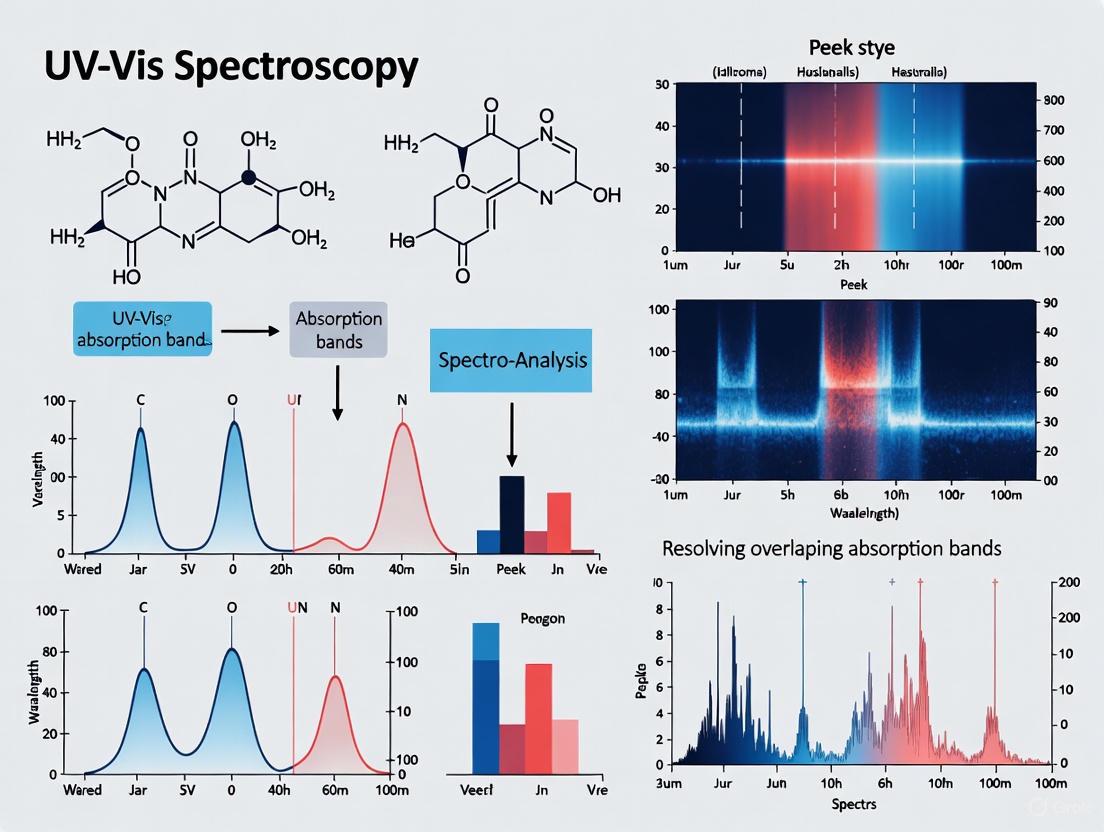
This article provides a complete resource for researchers and scientists on deconvoluting complex, overlapping bands in UV-Vis spectroscopy.
Resolving Overlapping UV-Vis Absorption Bands: A Comprehensive Guide from Foundations to Biomedical Applications
Abstract
This article provides a complete resource for researchers and scientists on deconvoluting complex, overlapping bands in UV-Vis spectroscopy. It covers the fundamental principles of electronic transitions and band formation, explores advanced mathematical and computational resolution techniques like Levenberg's method and DFT simulations, and addresses common pitfalls and optimization strategies for quantitative analysis. A dedicated section on validation and comparative analysis, illustrated with a case study on hemoglobin quantification, offers practical insights for ensuring accuracy in characterizing chemical equilibria, biomolecules, and pharmaceuticals, directly supporting rigorous drug development and clinical research.
The Fundamentals of UV-Vis Band Overlap: Why It Happens and What It Reveals
Core Principles of Electronic Transitions and Chromophores
Core Theory
What are electronic transitions and chromophores?
Electronic transitions occur when a molecule absorbs ultraviolet or visible radiation, causing an electron to jump from a lower-energy molecular orbital to a higher-energy one [1]. The energy required for this transition corresponds to specific wavelengths of light [2].
A chromophore is the functional group within a molecule responsible for absorbing light in the UV-Vis region [2]. Common chromophores include C=C, C=O, and aromatic rings. The structure of the chromophore, especially the presence of conjugation, directly influences the energy needed for electronic transitions [3].
What are the primary types of electronic transitions?
The table below summarizes the four primary types of electronic transitions relevant to organic molecules [1] [4].
Table 1: Characteristics of Electronic Transitions in UV-Vis Spectroscopy
| Transition Type | Electrons Involved | Typical λmax Range | Molar Absorptivity (ε) [L·mol⁻¹·cm⁻¹] | Example Compounds |
|---|---|---|---|---|
| σ → σ* | Sigma-bonding electrons | < 200 nm (High energy) | Very High | Methane, other alkanes |
| n → σ* | Non-bonding electrons | 150 - 250 nm | Medium (100 - 3000) | Saturated compounds with O, N, S, halogens |
| π → π* | Pi-bonding electrons | 200 - 700 nm (Conjugated systems) | High (1,000 - 10,000+) | Alkenes, alkynes, carbonyls, aromatics |
| n → π* | Non-bonding electrons | ~300 nm (Low energy) | Low (10 - 100) | Compounds with C=O, C≡N, N=O |
For organic and biological chemists, transitions of n or π electrons to the π* excited state are most experimentally convenient, as their absorption peaks fall within the standard UV-Vis range (200-700 nm) [1].
Troubleshooting Guides
Resolving Overlapping Absorption Bands
A common challenge in research, such as in the quantitative analysis of tautomeric equilibria, is deconvoluting overlapping UV-visible absorption bands [5].
Table 2: Methodology for Resolving Overlapping Absorption Bands
| Step | Action | Technical Details | Expected Outcome |
|---|---|---|---|
| 1 | Confirm Overlap | Collect spectra of individual pure components (if available) under identical solvent, pH, and temperature conditions. | Identifies the specific wavelengths where band overlap occurs. |
| 2 | Optimize Environment | Systematically vary solvent polarity [1] and sample pH [3]. | Induces bathochromic/hypsochromic shifts that may separate bands. |
| 3 | Record Full Spectrum | Ensure the instrument collects high-resolution data across a broad enough range. | Provides a complete dataset for mathematical analysis. |
| 4 | Apply Mathematical Analysis | Use specialized software for derivative spectroscopy or deconvolution algorithms [5]. | Resolves the composite spectrum into its individual component bands. |
Addressing Sample and Instrumentation Problems
Table 3: Troubleshooting Common UV-Vis Spectroscopy Issues
| Problem | Possible Cause | Solution | Prevention Tip |
|---|---|---|---|
| Unexpected Peaks | Contaminated sample or dirty cuvette [6]. | Thoroughly clean cuvettes with compatible solvents. Prepare a fresh sample. | Handle cuvettes with gloved hands and use high-purity reagents. |
| Noisy or Unstable Absorbance | Instrument lamp not warmed up, low light source intensity, or contaminated cuvette [6] [7]. | Allow lamp to warm up for 20+ minutes (tungsten/halogen). Ensure cuvette clean path is clear. | Follow manufacturer's warm-up procedure. Calibrate with blank before measurements [7]. |
| Signal Too Weak/Strong | Sample concentration is too low or too high [6]. | Concentrate or dilute sample. Use a cuvette with a longer or shorter path length. | Aim for an absorbance between 0.1 and 1.0 AU for optimal results [7]. |
| Non-Linear Beer's Law Plot | Instrumental stray light, chemical associations/dissociations, or overly high concentration [4] [7]. | Ensure monochromatic light, check for chemical stability (e.g., pH), and dilute sample. | Use concentrations typically below 0.01 M to minimize molecular interactions [3]. |
The following workflow can help systematically diagnose and resolve common instrument and sample-related issues:
Frequently Asked Questions (FAQs)
Q1: Why does my sample's absorption maximum (λmax) shift when I change the solvent? The polarity of the solvent interacts differently with the ground and excited states of the chromophore. For n→π* transitions, increasing solvent polarity typically causes a blue shift (shorter wavelength) because the ground state is stabilized by solvation of the lone pair electrons. For π→π* transitions, a red shift (longer wavelength) is often observed because the excited state is more stabilized than the ground state [1] [3].
Q2: What is conjugation and how does it affect the spectrum? Conjugation occurs when pi bonds are separated by only one single bond, creating a system of delocalized electrons [8]. This delocalization lowers the energy gap between the HOMO and LUMO. A smaller energy gap requires less energy for an electronic transition, resulting in absorption at a longer wavelength (a bathochromic shift) [8] [3]. For example, beta-carotene, with its 11 conjugated double bonds, absorbs blue light and appears orange [2].
Q3: What is the difference between a chromophore and an auxochrome? A chromophore is a functional group that itself absorbs light in the UV-Vis region (e.g., C=C, C=O). An auxochrome is a functional group (often with lone pairs like -OH, -NH₂) that, when attached to a chromophore, modifies its absorption. Auxochromes typically cause a bathochromic shift to a longer wavelength and can increase the intensity of absorption (hyperchromic effect) [4].
Q4: My absorbance readings are unstable. What should I check first? First, ensure your instrument's light source has warmed up sufficiently (20+ minutes for tungsten/halogen lamps) [6]. Then, check that the cuvette is clean, free of scratches, and properly positioned in the beam path. Finally, verify the sample concentration is within the ideal range (absorbance between 0.1 and 1.0) and that solvent evaporation is not occurring [6] [7].
The Scientist's Toolkit
Table 4: Essential Research Reagents and Materials for UV-Vis Spectroscopy
| Item | Function/Application | Critical Specifications |
|---|---|---|
| Quartz Cuvettes | Holds liquid sample for analysis. | Transmission down to ~200 nm; reusable with various path lengths (e.g., 1 cm). |
| Solvents (UV Grade) | Dissolve analyte without interfering with absorption. | High purity, "UV Grade" with low absorbance in UV region (e.g., acetonitrile, hexane). |
| pH Buffers | Control the ionization state of analytes, crucial for studying tautomers or ionic species [3]. | Non-absorbing in spectral range of interest; must not precipitate or react with analyte. |
| Standard Reference Materials | Validate instrument performance and wavelength accuracy. | Materials with known and sharp absorption peaks (e.g., holmium oxide filter). |
| Deuterium or Tungsten Lamp | Provides light source across UV and visible regions, respectively [4]. | Ensure lamp life is within specifications and it is properly warmed up before use. |
Experimental Protocol: Analyzing a Tautomeric Equilibrium
This protocol provides a detailed methodology for studying tautomeric equilibria, a classic example of resolving overlapping absorption bands [5].
Title: Quantitative Analysis of a Keto-Enol Tautomeric Equilibrium Using UV-Vis Spectroscopy.
Principle: Tautomers are structural isomers that readily interconvert. The keto and enol forms will have distinct chromophores and thus different absorption maxima (λmax). The equilibrium can be shifted by altering solvent polarity or pH, allowing for the isolation and analysis of each form's spectral signature.
Procedure:
- Sample Preparation: Prepare a stock solution of the tautomeric compound (e.g., acetylacetone) in a UV-grade solvent of low polarity (e.g., cyclohexane).
- Initial Spectrum: Fill a clean quartz cuvette with the solution and collect a baseline-corrected absorption spectrum from 220 nm to 350 nm.
- Solvent Perturbation: Prepare a second solution of the compound in a more polar, protic solvent (e.g., methanol-water mixture). Collect its absorption spectrum under identical conditions.
- pH Perturbation (if applicable): For tautomers sensitive to pH, prepare solutions buffered at different pH levels (e.g., pH 4 and pH 9) and collect their spectra.
- Data Analysis: Use the spectra to identify the λmax for each tautomer. The keto form typically absorbs at shorter wavelengths, while the enol form, due to extended conjugation, absorbs at longer wavelengths. The relative concentration of each tautomer can be determined from the absorbance at their respective λmax and their known molar absorptivities.
Key Observations:
- In non-polar solvents, the enol form is often favored, showing a stronger π→π* absorption band at longer wavelengths.
- In polar protic solvents, the keto form may be stabilized, increasing the intensity of its n→π* band.
- A clear isosbestic point (a wavelength where absorbance is constant regardless of the tautomer ratio) in the series of spectra indicates an equilibrium between two species.
Frequently Asked Questions
What are the fundamental parameters of a UV-Vis absorption band? Every electronic transition in a UV-Vis spectrum appears as a band characterized by three fundamental parameters: the position (wavelength of maximum absorption, λ_max), the intensity (measured by absorbance and quantitatively expressed by the molar extinction coefficient, ε), and the width (typically measured as the full width at half maximum, FWHM) [9]. These parameters are used to estimate fundamental transition characteristics and are essential for quantitative analysis [9].
Why is accurately defining these parameters critical for analyzing overlapping bands? In complex spectra, individual component bands are often strongly overlapped and can have different widths, making it difficult to estimate their number and individual characteristics [9] [10]. Correctly resolving these overlapping bands to determine their position, intensity, and width is a necessary step to extract meaningful quantitative information about the sample, such as in the study of tautomeric equilibria or the analysis of multi-component mixtures [5] [9].
What are the most common challenges in resolving overlapping bands? The main challenges include [9]:
- Correctly estimating the number of overlapping bands contributing to the overall spectral envelope.
- Dealing with experimental noise, which can interfere with mathematical resolution methods.
- Accounting for or correcting an artificial baseline.
- Ensuring the efficiency and stability of the computational fitting procedure.
Troubleshooting Guides
Problem: Inconsistent or inaccurate band parameter values upon repeated analysis.
| Potential Cause | Solution |
|---|---|
| High Spectral Bandwidth | Ensure the instrument's spectral bandwidth is significantly narrower than the width of the absorption peak being measured. A wider bandwidth can lead to lower resolution and inaccurate measurements of extinction coefficient and band shape [11]. |
| Stray Light | Use a instrument with a double monochromator for measurements requiring high absorbance range (>2 AU). Stray light causes significant errors, especially at high absorbances, by reporting an incorrectly low absorbance [11]. |
| Wavelength Error | Conduct quantitative measurements at a wavelength close to the absorbance peak (λ_max), where the rate of change of absorbance is lowest. This minimizes inaccuracies from small errors in wavelength calibration [11]. |
| Deviations from Beer-Lambert Law | At high concentrations, absorption bands can saturate, causing absorption flattening and non-linear responses. Dilute the sample or use a shorter path length to bring the absorbance into a linear range [11]. |
Problem: Failure to achieve a good fit when deconvoluting overlapping bands.
| Potential Cause | Solution | |
|---|---|---|
| Incorrect Initial Estimates | The success of iterative fitting algorithms (like Levenberg's method) is highly dependent on the initial input values for position, intensity, and width. Use prior knowledge or derivative spectra to make informed initial guesses [10]. | |
| Wrong Number of Bands | An underestimation or overestimation of the number of underlying components will prevent a physically meaningful fit. Use statistical methods or singular value decomposition (SVD) available in software like `a | e` to help determine the number of components [12]. |
| Unaccounted for Baseline | A sloping or curved baseline can distort the fitted bands. Always include a baseline correction function (e.g., linear or polynomial) in the deconvolution model [9]. |
Experimental Protocols for Band Resolution
Methodology for the Mathematical Resolution of Overlapping Bands
The following logical algorithm provides a step-by-step guide for resolving individual bands from a complicated, overlapped spectrum [9] [10].
Quantitative Analysis Using Resolved Band Parameters
Once the pure component bands are resolved, their intensities (absorbance or ε) can be used for quantitative analysis. The relationship between these parameters for a single component is governed by the Beer-Lambert law [11]:
Table 1: Core Band Parameters and Their Interrelationship via the Beer-Lambert Law
| Parameter | Symbol & Units | Relationship & Significance |
|---|---|---|
| Position | λ_max (nm) | Identifies the energy of the electronic transition; characteristic of the chromophore and its environment [9] [11]. |
| Intensity | A (Absorbance Units), ε (M⁻¹cm⁻¹) | A = ε c L The measured absorbance (A) is directly proportional to the concentration (c) and path length (L), with ε being the intrinsic molar absorptivity [11]. |
| Width | Δν₁/₂ or FWHM (cm⁻¹ or nm) | Related to the lifetime of the excited state and reflects the heterogeneity of the sample's microenvironment [9]. |
For a mixture of K components, the mass spectrum observed at any point is a linear combination of the pure component spectra, weighted by their concentrations [13]. This same principle applies to UV-Vis spectra of multi-component solutions, where the absorbance at any wavelength is the sum of contributions from all absorbing species.
Table 2: Key Software and Mathematical Tools for Band Analysis
| Tool Name | Function | Relevance to Band Parameter Definition | |
|---|---|---|---|
| a | e - UV-Vis-IR Spectral Software [12] | General spectral analysis. | Performs operations like singular value decomposition (SVD) to determine the number of components and can fit Gaussians to spectra, directly aiding in the resolution of overlapping bands. |
| Chemissian [14] | Electronic structure and spectra analysis. | Allows visualization and interpretation of UV-Vis spectra from computational outputs (e.g., TDDFT). Helps link experimental band parameters to theoretical electronic transitions. | |
| Levenberg's Method [10] | Non-linear least squares algorithm. | A robust iterative procedure used to optimize the parameters (position, intensity, width) of individual bands during the deconvolution of a complex spectral envelope. | |
| Statistical Overlap Theory (SOT) [15] | Models peak crowding in separations. | Provides a theoretical framework for understanding the probability of peak overlap, which is directly analogous to the challenge of resolving overlapping absorption bands in spectroscopy. |
The relationships between the core concepts, data, and analytical goals in defining band parameters can be visualized as follows:
Fundamental Concepts of Band Overlap
What is Band Overlap and Why Does It Occur?
In UV-Vis spectroscopy, band overlap refers to the phenomenon where the absorption bands of two or more different chemical species in a mixture, or multiple electronic transitions from a single complex molecule, are insufficiently separated in the wavelength axis. This results in a single, broadened, or poorly resolved absorption peak in the measured spectrum [10]. Analyzing such spectra is a complicated task because these absorption bands can have different half-band widths, and their number is often difficult to estimate with confidence [10].
This overlap obscures the unique "fingerprint" of individual components, making it challenging to accurately identify substances or determine their concentrations. In the context of your research, resolving this overlap is critical for obtaining meaningful data on molecular structure and environment [10].
Key Molecular and Systemic Interactions Leading to Overlap
The root causes of band overlap often lie in the fundamental chemical and physical interactions within your sample. The table below summarizes the primary sources.
Table 1: Common Sources of Band Overlap in Chemical and Biological Systems
| Source of Overlap | Description | Common Examples in Research |
|---|---|---|
| Multiple Chromophores | A molecule contains several light-absorbing groups whose individual electronic transitions occur at similar energies. | Proteins with aromatic amino acids (Tryptophan, Tyrosine); drug molecules with complex conjugated systems [16]. |
| Complex Mixtures | The simultaneous presence of multiple absorbing species in a solution, without chemical interaction between them. | Biological buffers containing nucleotides (e.g., ATP) and proteins [16]; mixtures of dyes or metabolites [16]. |
| Molecular Aggregation | Chromophores stack together through non-covalent interactions (e.g., π-π stacking), altering their individual absorption properties. | Dye aggregates; π-π stacked nucleobases in DNA [17]; supramolecular assemblies [17]. |
| Hydrogen Bonding | H-bonding with the solvent or between molecules can shift the energy levels of chromophores, leading to broadening and shifting of peaks. | DNA base pairing (e.g., G-C, A-T) [17]; solute-solvent interactions in aqueous solutions [17]. |
Methodologies for Resolving Overlapping Bands
Successfully deconvoluting overlapping bands requires a systematic approach, from sample preparation to advanced data analysis. The following workflow outlines the key steps in this process.
Experimental Protocol for Sample Preparation
Proper sample preparation is the first and most crucial line of defense against band overlap issues [6].
- Optimize Concentration: Aim for an absorbance value between 0.2 and 1.0 AU (Absorbance Units) at the peak of interest. Absorbance readings become unstable and non-linear above 1.0, which can exacerbate overlap interpretation problems [18] [19]. If the absorbance is too high, dilute your sample.
- Select Appropriate Solvent: Ensure the solvent does not absorb significantly in your wavelength range of interest. For UV work below 210 nm, use high-purity UV-grade solvents [6] [19].
- Ensure Sample Clarity: For solution samples, filter or centrifuge to remove any particulate matter that can cause light scattering, which distorts the baseline and absorption profile [19].
- Use Correct Cuvettes: Always use high-quality quartz cuvettes for UV-Vis measurements, as they transmit both UV and visible light. Plastic or glass cuvettes can absorb UV light and introduce errors [6] [18].
Mathematical Resolution Protocol: Levenberg's Method
When instrumental and sample optimization are insufficient, mathematical techniques are required. One powerful approach is the use of Levenberg's method, which is an algorithm for resolving individual bands from a complex, overlapped spectrum [10].
- Data Collection: Collect a high-resolution absorbance spectrum of the sample containing the overlapped bands.
- Initial Parameter Estimation: Make an initial estimate of the number of underlying bands, and their approximate position, height, and width. The number of bands can be difficult to estimate and may require prior knowledge of the system [10].
- Curve Fitting: The algorithm iteratively adjusts the parameters (position, amplitude, width) of individual band shapes (e.g., Gaussian or Lorentzian curves) to find the best fit to the measured, overlapped spectrum.
- Validation: The resolved spectrum (sum of the fitted individual bands) is compared to the original measured spectrum. The process repeats until the difference between them is minimized.
This method has been successfully applied to resolve the vibrational structured long-wavelength bands of molecules like trans-stilbene and its derivatives [10].
Advanced Technique: UV/Vis Diffusion-Ordered Spectroscopy (UV/Vis-DOSY)
A novel method to separate overlapping bands is UV/vis-DOSY, which combines principles from NMR with optical spectroscopy [16]. This technique separates species by their hydrodynamic radius (size) while simultaneously providing their UV/vis spectrum.
- Principle: A sample solution and pure solvent are placed in contact in a specialized cell. After the flow is stopped, molecules diffuse from the sample zone into the solvent zone at a rate inversely proportional to their size (via the Stokes-Einstein relation). The time-dependent absorption spectrum is recorded in the solvent zone [16].
- Data Output: The result is a 2D spectrum with absorption wavelength on one axis and diffusion coefficient (size) on the other. The UV/vis spectrum of a mixture is separated into the spectra of its different species, sorted by size [16].
- Application Example: This method can clearly resolve the individual spectra of a mixture of rhodamine B and methylene blue dyes, which have different sizes and diffuse at different rates, even though their absorption bands overlap in a conventional spectrum [16].
The Scientist's Toolkit: Essential Research Reagent Solutions
Having the right materials is fundamental for reliable spectroscopy and effective band resolution.
Table 2: Key Reagents and Materials for Band Resolution Experiments
| Item | Function in Experiment | Key Considerations |
|---|---|---|
| Quartz Cuvettes | Holds liquid sample in the light path. | Essential for UV range measurements; ensure cleanliness and correct path length (e.g., use shorter path length for high-concentration samples) [6] [18]. |
| High-Purity Solvents | Dissolves the analyte without interfering. | Use HPLC-grade or better; check the solvent's UV-cutoff wavelength to ensure it is transparent in your measurement region [19]. |
| Certified Reference Standards | For instrument calibration and validation. | Use certified materials like Holmium Oxide for wavelength verification. Ensures instrument performance and data accuracy [19]. |
| Buffer Solutions | Maintains biological molecules in a stable, native state. | The buffer should not absorb in the measured range. Phosphate buffers are often a good choice for UV studies [19]. |
| Syringe Pump & Flow Cell (for UV/vis-DOSY) | Creates the initial solvent-solution boundary for diffusion measurements. | Enables the use of advanced separation techniques like UV/vis-DOSY for complex mixtures [16]. |
Troubleshooting FAQs for Band Overlap Issues
The absorbance peaks in my spectrum of a biological mixture are broad and poorly resolved. What should I check first?
First, verify your sample concentration. A highly concentrated sample can lead to peak broadening and non-linear absorbance (deviating from the Beer-Lambert Law), making bands appear to merge. Dilute your sample to bring the maximum absorbance below 1.0 AU, ideally between 0.2 and 1.0, and recollect the spectrum [18] [19]. Second, check for sample clarity. Turbid solutions scatter light, creating a sloping baseline that distorts the true absorption profile. Filter or centrifuge your sample to remove any particulates [19].
I am using a common buffer, but my baseline is very high in the UV region. Why?
Many common biochemical buffers (e.g., Tris) or additives absorb strongly in the UV range below 230 nm. This high background absorption can mask the analyte's signal and create apparent overlap. Prepare a fresh blank using your exact buffer solution and ensure you are using a buffer with low UV absorbance for your wavelength range of interest [19].
The mathematical deconvolution of my overlapped band is not converging. What could be wrong?
The most common issue is an incorrect initial estimate of the number of component bands. The algorithm needs a reasonable starting point to find the optimal fit. Re-evaluate your system:
- Do you have prior knowledge (e.g., from literature or HPLC) about how many species are likely present?
- Could the overlap be due to more components than you initially assumed? Using an advanced technique like UV/vis-DOSY can provide an independent measurement of the number of species present based on their size, which can then be used to constrain the mathematical fitting [10] [16].
After resolving the bands, how can I validate that the individual peaks are real and not mathematical artifacts?
Validation is critical. If possible, compare your resolved spectra with the known absorption spectra of the pure compounds run under identical conditions (same solvent, pH, etc.). Another powerful method is to use an orthogonal technique, such as chromatography (HPLC-UV), to physically separate the components and measure their individual UV spectra, confirming the results from your mathematical deconvolution [16].
A fundamental challenge in UV-Vis spectroscopy is accurately analyzing samples where multiple chemical species, such as tautomers, coexist and contribute to a single, composite absorption spectrum [20]. The strong overlap of individual spectral bands can obscure crucial information about each component's identity, concentration, and electronic structure. This technical guide provides targeted methodologies and troubleshooting advice for researchers aiming to resolve these complex spectra, with a particular focus on systems involving tautomerism—a form of isomerism where species readily interconvert via proton transfer, leading to decisive modifications in chemical bonding and functionality [20].
Mathematical Resolution of Overlapping Bands
Electronic transitions in a spectrum are characterized by three fundamental parameters: position, intensity, and band width [9]. The mathematical resolution of a composite spectrum into its individual components relies on determining the number of overlapping bands and optimizing these parameters for each component to reconstruct the observed signal.
Key Steps and Challenges:
- Band Number Estimation: The first and often most difficult step is estimating the correct number of underlying bands. Initial guesses can be informed by chemical knowledge of the system or by examining second derivatives of the spectrum.
- Noise Management: The presence of noise in experimental data can severely impact the accuracy of the resolved bands. Smoothing algorithms or weighted least-squares fitting are often employed to mitigate this issue [9].
- Baseline Correction: An artificial or incorrectly fitted baseline can introduce significant errors. It is crucial to identify and subtract the baseline before or during the decomposition process [9].
- Computational Efficiency: The computing procedure must be efficient enough to handle the non-linear optimization problem, especially when dealing with a large number of spectral data points or multiple components [9].
Algorithmic Approach: A logical algorithm using the Levenberg-Marquardt method is highly effective for this non-linear curve-fitting problem [10]. This method combines the steepest descent and Gauss-Newton algorithms for robust convergence.
Table 1: Quantitative Parameters for Resolved Bands of trans-Stilbene Derivatives [10]
| Compound | Band Assignment | λ_max (nm) | Absorbance | Half-Band Width (nm) |
|---|---|---|---|---|
| trans-Stilbene | Band 1 | ~300 | Varies | ~30 |
| Band 2 | ~320 | Varies | ~35 | |
| Derivative A | Band 1 | ~305 | Varies | ~32 |
| Band 2 | ~325 | Varies | ~36 | |
| Derivative B | Band 1 | ~310 | Varies | ~31 |
| Band 2 | ~330 | Varies | ~37 |
Experimental Protocols for Tautomeric Systems
Tautomeric equilibria, such as the keto-enol equilibrium in 3-hydroxypyridine (3HP), present a classic challenge where the individual UV-Vis absorption bands of tautomers overlap strongly [20]. Traditional methods involve perturbing the equilibrium by changing solvents or pH to detect spectral variations, which are then decomposed using statistical methods [20].
Advanced Spectroscopic Technique: Resonant Inelastic X-ray Scattering (RIXS)
RIXS offers a more direct method to disentangle the spectral contributions of individual tautomers in a mixture [20].
Principle: The technique exploits the large chemical shift in core-level excitation energies (e.g., at the nitrogen K-edge) between the two tautomers. By tuning the X-ray energy to the specific absorption resonance of one tautomer, the subsequent emission (RIXS) spectrum provides a "pure" map of its valence electronic excitations [20].
Methodology:
- Sample Preparation: Prepare an aqueous solution of 3HP, which exists as a nearly 1:1 mixture of enol and keto tautomers [20]. The sample is typically introduced as a liquid jet for measurement [20].
- Data Collection:
- Tune the incident X-ray beam to the specific π* resonance of the enol tautomer and collect a RIXS spectrum.
- Tune the incident X-ray beam to the specific π* resonance of the keto tautomer and collect a second RIXS spectrum.
- This generates a 2D map where regions of emission intensity are associated with each tautomer [20].
- Data Interpretation:
- The RIXS spectra for each tautomer contain transitions from occupied molecular orbitals into the lowest unoccupied molecular orbital (LUMO).
- Use scattering anisotropy (comparing spectra from vertically and horizontally polarized X-rays) to assign peaks to transitions from π or σ bonding manifolds [20].
- Key Insight: The presence of a strong nitrogen lone-pair peak (~5 eV energy loss) is a clear signature of the enol form, which is absent in the keto form where the lone pair is involved in an N-H bond [20].
Troubleshooting FAQs
Q1: My UV-Vis spectrum of a carbonyl compound shows a weak absorbance at ~275 nm and a very strong one below 200 nm. What transitions do these represent? A1: The weak band at ~275 nm is an n→π* transition, where an electron from a non-bonding orbital on the oxygen is promoted to the π* orbital of the C=O group. The strong band below 200 nm is a π→π transition within the C=O bond. The n→π transition is weak because the non-bonding and π* orbitals have poor spatial overlap [21].
Q2: How does conjugation affect the UV-Vis spectrum of a molecule? A2: Increasing conjugation decreases the energy gap (ΔE) between the highest occupied molecular orbital (HOMO) and the lowest unoccupied molecular orbital (LUMO). This results in a bathochromic shift (red shift), meaning the wavelength of maximum absorbance (λmax) increases and moves toward the visible region. For example, extending conjugation from ethene (λmax = 174 nm) to butadiene (λ_max = 217 nm) causes a clear red shift [22].
Q3: When using computational chemistry to predict a UV-Vis spectrum, how do I ensure I'm calculating an absorption spectrum and not an emission spectrum? A3:
- Absorption spectra are obtained by performing a time-dependent DFT (TD-DFT) calculation on the optimized ground-state geometry.
- Emission spectra are obtained by performing a TD-DFT calculation on the optimized excited-state geometry. If your calculation uses the ground-state geometry, the spectrum generated by your software (e.g., GaussView) is the absorption spectrum. The software might display both, but only the absorption spectrum is meaningful in this context [23].
Advanced Techniques: In Situ UV-vis-NIR Spectroscopy
For studying catalysts or reactions under operational conditions, in situ UV-vis-NIR spectroscopy is a powerful tool. It spans a broad range (200-2500 nm) to probe various electronic and vibrational transitions [24].
Table 2: UV-vis-NIR Spectral Regions and Transition Information
| Spectral Region | Wavelength Range | Typical Transitions Observed | Information Gained |
|---|---|---|---|
| Ultraviolet (UV) | 200 - 400 nm | Ligand-to-Metal Charge Transfer (LMCT), Metal-to-Ligand Charge Transfer (MLCT), π→π* | Structural and electronic information, oxidation states [24]. |
| Visible (Vis) | 400 - 700 nm | d-d transitions of Transition Metal Ions (TMI) | Coordination environment of metal centers [24]. |
| Near Infrared (NIR) | 700 - 2500 nm | Overtones and combination bands of O-H, C-H, N-H vibrations | Probing structural defects and molecular interactions [24]. |
Application: This technique is widely used in heterogeneous catalysis to monitor active sites in real-time. For example, it can track changes in the oxidation state of copper or iron ions within a zeolite catalyst during a reaction, providing insights into the reaction mechanism and kinetics [24].
The Scientist's Toolkit: Essential Research Reagents & Materials
Table 3: Key Reagents and Computational Tools for Spectral Analysis
| Item / Reagent | Function / Role in Analysis |
|---|---|
| 3-Hydroxypyridine (3HP) | A prototypical model compound for studying keto-enol tautomerism in aqueous solution [20]. |
| Solvent Mixtures (various polarities) | Used to perturb tautomeric equilibria, allowing for the observation of spectral shifts for individual components [20]. |
| Levenberg-Marquardt Algorithm | A key non-linear optimization algorithm for resolving individual bands from a complex, overlapped spectrum [10]. |
| TD-DFT (Time-Dependent DFT) | A computational method used to predict and assign electronic excitations and UV-Vis spectra from first principles [23]. |
| InChI Identifier | A standardized, non-proprietary identifier for chemical substances, crucial for unambiguous data sharing and compound registration in databases [25] [26]. |
Advanced Techniques for Spectral Deconvolution: From Algorithms to Practical Workflows
Mathematical Foundations for Resolving Overlapping Bands
In UV-Vis spectroscopy, the analysis of complex mixtures often results in overlapping absorption bands, where the spectra of individual components are superimposed. This presents a significant challenge for accurate qualitative and quantitative analysis. The mathematical resolution of these overlapping bands is therefore a critical foundation in spectroscopic research, enabling researchers to extract meaningful information about individual components from a composite signal. This guide outlines the core principles, methodologies, and practical protocols for effectively resolving such spectral overlaps, with a focus on applications in pharmaceutical analysis and drug development.
Core Mathematical Principles and Techniques
The resolution of overlapping UV-Vis absorption bands relies on the fact that individual electronic transitions in a spectrum are characterized by three fundamental parameters: position, intensity, and width [9]. The primary challenge lies in accurately determining the number of overlapping bands, dealing with spectral noise, and employing efficient computational procedures to deconvolute the composite signal [9].
The following table summarizes the key mathematical techniques used for resolving binary mixtures, along with their central principle and a common application challenge.
Table 1: Overview of Key Techniques for Resolving Overlapping Spectra
| Technique | Fundamental Principle | Typical Application Challenge |
|---|---|---|
| Derivative Spectrophotometry | Uses first or higher-order derivatives of absorbance with respect to wavelength to enhance minor spectral features and suppress broad-band background interference [27]. | Higher-order derivatives amplify high-frequency noise, requiring a balance between resolution enhancement and signal-to-noise ratio [27]. |
| Simultaneous Equation Method | Solves a set of linear equations based on the absorbance of each component at its wavelength of maximum absorption (λmax) [28]. | Requires that the absorptivities of both drugs are known at the two selected wavelengths and that they obey Beer-Lambert's law [28]. |
| Dual Wavelength Method | Selects two wavelengths where the interfering component has the same absorbance (isoabsorptive point), thus canceling its contribution [28]. | Finding a suitable pair of wavelengths where the analyte shows a significant difference in absorbance while the interferent does not can be difficult in highly overlapping spectra [28]. |
| Ratio-based Methods (Ratio Difference, Ratio Derivative) | Uses the ratio of the absorption spectra of the mixture against a standard spectrum of one component to resolve the other component [28]. | The accuracy is highly dependent on the purity of the standard spectrum used as a divisor. |
| Bivariate Method | Employs linear calibration regressions at two optimally selected wavelengths for the simultaneous determination of both components in a mixture [28] [29]. | The selection of the two wavelengths is critical; Kaiser's method is often used to determine the optimal wavelength pair for the sensitivity matrix [29]. |
| Advanced Absorbance & Spectrum Subtraction | Mathematically subtracts the absorbed spectrum of one component from the mixture's spectrum to isolate the spectrum of the second component [28] [29]. | Requires prior knowledge of the exact concentration of the component to be subtracted, or the use of an isoabsorptive point to find the total concentration [29]. |
The logical relationship and primary application of these methods for resolving a binary mixture can be visualized in the workflow below.
Detailed Experimental Protocols
This section provides step-by-step methodologies for implementing key resolution techniques, using real analytical applications as models.
Protocol: Simultaneous Equation Method for Hydroxychloroquine and Paracetamol
This method is applied when the spectra of two components, Hydroxychloroquine (HCQ) and Paracetamol (PAR), overlap but each has a distinct λmax [28].
- Step 1: Obtain Pure Standard Solutions. Prepare known concentrations of pure HCQ and PAR in a suitable solvent (e.g., distilled water).
- Step 2: Record Absorbance Spectra. Scan the absorption spectra of both pure standard solutions within the 200-400 nm range.
- Step 3: Select Two Wavelengths. Choose the wavelength of maximum absorption (λmax) for each drug. In the HCQ/PAR model, these are 220 nm (λmax of HCQ) and 242.5 nm (λmax of PAR) [28].
- Step 4: Determine Absorptivity Values. Calculate the absorptivity (A 1%, 1 cm) for each drug at both selected wavelengths.
- Let
ax1andax2be the absorptivities of HCQ at 220 nm and 242.5 nm, respectively. - Let
ay1anday2be the absorptivities of PAR at 220 nm and 242.5 nm, respectively. - Reported values: ax1=0.0881, ax2=0.0339, ay1=0.0419, ay2=0.0521 [28].
- Let
- Step 5: Formulate Simultaneous Equations. For a mixture sample, measure the absorbance (A1 and A2) at the two selected wavelengths. The concentrations of HCQ (Cx) and PAR (Cy) in the sample are calculated using:
Cx = (A2*ay1 - A1*ay2) / (ax2*ay1 - ax1*ay2)Cy = (A1*ax2 - A2*ax1) / (ax2*ay1 - ax1*ay2)
- Validation Note: This method requires that the absorptivities of both drugs are known at the two selected wavelengths and that they obey Beer-Lambert's law across the working concentration range [28].
Protocol: Advanced Absorbance Subtraction (AAS) for Ciprofloxacin and Metronidazole
This protocol is designed to determine one component in a binary mixture by leveraging isoabsorptive points and wavelengths where the interferent shows equal absorbance [29].
- Step 1: Identify an Isoabsorptive Point. Scan the spectra of the individual components and the mixture to find a wavelength where both components have the same absorptivity. For Ciprofloxacin (CIP) and Metronidazole (MET), this point is at 291.5 nm [29]. The total concentration of the mixture (Ctotal) can be determined from this point.
- Step 2: Determine MET in the presence of CIP:
- Measure the absorbance of the mixture at the isoabsorptive point (291.5 nm) and at a second wavelength (250 nm) where CIP has the same absorbance as it does at 291.5 nm.
- The absorbance difference of CIP between these two wavelengths is zero. Therefore, any measured difference in the mixture's absorbance is directly proportional to the concentration of MET.
- Calculate the concentration of MET using a pre-established regression equation [29].
- Step 3: Determine CIP in the presence of MET:
- Measure the absorbance of the mixture at the isoabsorptive point (291.5 nm) and at a different second wavelength (345 nm) where MET has the same absorbance as it does at 291.5 nm.
- The absorbance difference of MET between these two wavelengths is zero. The measured difference is thus proportional only to CIP.
- Calculate the concentration of CIP using its specific regression equation [29].
Protocol: Obtaining and Using Derivative Spectra
Derivative spectroscopy is a powerful tool for resolving overlapping bands and eliminating baseline shifts [27] [30].
- Step 1: Generate the Zero-Order Spectrum. Record the normal absorbance spectrum (zero-order) of the sample mixture.
- Step 2: Calculate the Derivative. Modern spectrophotometers use mathematical differentiation to compute the first or higher-order derivatives of the absorbance spectrum with respect to wavelength.
- First Derivative (¹D): Plots the rate of change of absorbance (dA/dλ). It crosses zero at the same wavelength as the λmax of the absorbance band in the zero-order spectrum. It is effective in eliminating constant baseline interference [27].
- Second Derivative (²D): Shows a negative peak (minimum) at the same wavelength as the λmax of the zero-order band. It is highly effective in resolving closely spaced or overlapping peaks [27] [30].
- Step 3: Quantitative Measurement. For quantification, use the peak-to-trough amplitude (for even-order derivatives) or the distance from a peak to the zero line (for odd-order derivatives) at a specific wavelength. For example, the first derivative amplitude at 329 nm has been used to determine Hydroxychloroquine where Paracetamol shows zero crossing and thus no interference [28].
Troubleshooting Common Experimental Issues
Even with robust mathematical techniques, researchers often encounter practical problems. The following guide addresses common issues and their solutions.
Table 2: Troubleshooting Guide for Resolving Overlapping Bands
| Problem | Possible Cause | Recommended Solution |
|---|---|---|
| High noise in derivative spectra | Amplification of high-frequency noise during the differentiation process [27]. | Apply smoothing functions (e.g., Savitzky-Golay filter) to the zero-order spectrum before derivative calculation. Optimize the smoothing parameters to balance noise reduction and signal preservation [27]. |
| Deviation from Beer-Lambert's Law | High analyte concentration leading to molecular interactions or detector non-linearity; presence of stray light [19]. | Dilute the sample to bring the absorbance into the ideal range (0.2–1.0 AU). Ensure the instrument is well-maintained and calibrated for stray light [19]. |
| Poor resolution of closely overlapping bands | The overlapping bands are too broad or their λmax values are too close relative to their half-widths [10]. | Switch to a higher-order derivative (e.g., second or fourth derivative) which provides better band narrowing. Alternatively, combine derivative techniques with ratio methods [27]. |
| Inaccurate results with subtraction methods | Incorrect concentration estimate of the component being subtracted, or spectral contribution from an unknown interferent. | Use an isoabsorptive point to accurately determine the total concentration before subtraction. Validate the method by analyzing samples with known compositions [29]. |
| Significant baseline drift or shift | Fluctuations in the light source intensity, temperature changes in optical components, or dirty sample cuvettes [19]. | Use a double-beam instrument that compensates for real-time baseline drift. Ensure proper instrument warm-up and use matched, clean quartz cuvettes. Derivative spectroscopy can also help correct for baseline shifts [27] [19]. |
The Scientist's Toolkit: Essential Reagents and Materials
The following table lists key materials and their functions for conducting experiments on resolving overlapping UV-Vis bands, based on cited protocols.
Table 3: Essential Research Reagents and Materials
| Item | Specification / Function |
|---|---|
| Double-Beam UV-Vis Spectrophotometer | Equipped with software capable of mathematical processing (derivative calculation, spectral subtraction, etc.) [28] [29]. |
| Quartz Cuvettes | 1 cm pathlength; for holding liquid samples without absorbing in the UV range [28] [29]. |
| Reference Standards | High-purity analytes (e.g., Hydroxychloroquine, Ciprofloxacin) for establishing calibration curves and absorptivity values [28] [29]. |
| Distilled / Deionized Water | A common solvent for preparing stock and working standard solutions, especially for water-soluble pharmaceuticals [28] [29]. |
| Volumetric Flasks | For precise preparation and dilution of standard and sample solutions (e.g., 10 mL flasks) [28] [29]. |
| Certified Reference Materials | Holmium oxide or other certified filters for regular wavelength accuracy calibration of the spectrophotometer [19]. |
The decision-making process for selecting an appropriate resolution method based on the characteristics of the spectral overlap and available data is summarized below.
Frequently Asked Questions (FAQs)
Q1: What is the main advantage of using derivative spectroscopy over the simultaneous equation method? A1: Derivative spectroscopy excels at eliminating baseline shifts and enhancing minor spectral features, which is particularly useful for detecting shoulder peaks in heavily overlapping bands. The simultaneous equation method is more straightforward but requires well-resolved λmax points and is susceptible to errors from baseline drift [27] [30] [28].
Q2: Can these mathematical methods be applied to systems with more than two overlapping components? A2: While the principles extend to multi-component systems, the complexity increases significantly. Techniques like multivariate calibration (e.g., Principal Component Regression or Partial Least Squares) are more suitable for three or more components, as they can handle higher levels of spectral overlap and interaction [9].
Q3: How critical is instrument calibration for these resolution techniques? A3: Highly critical. Regular calibration of wavelength accuracy (using, e.g., holmium oxide filters) and absorbance accuracy is essential. Uncalibrated instruments can lead to shifts in λmax and erroneous absorptivity values, which directly impact the accuracy of all resolution methods, especially those relying on precise wavelength selection like the dual wavelength and simultaneous equation methods [19].
Q4: What is the simplest method to start with for a binary mixture with partial overlap? A4: The simultaneous equation method is often the simplest to implement initially, provided the two components have distinct and clear λmax values. It requires only the measurement of absorbance at two wavelengths and solving two linear equations, making it easy to compute and validate [28].
In UV-Vis spectroscopy, the analysis of complex mixtures is often complicated by strongly overlapped absorption bands. These bands can have different half-band widths, and their number is frequently difficult to estimate, making resolution a challenging task [10]. Computational methods, particularly optimization algorithms like Levenberg's, have become indispensable for extracting meaningful quantitative information from these complex spectral datasets. When combined with artificial neural networks (ANNs) and proper spectral preprocessing, these approaches enable researchers to resolve individual components in pharmaceutical mixtures, environmental samples, and biological matrices with remarkable accuracy [31] [32].
Core Algorithm Guide: Levenberg-Marquardt and Alternatives
Levenberg-Marquardt Algorithm Fundamentals
The Levenberg-Marquardt (LM) algorithm is a standard nonlinear least-squares optimization technique that combines gradient descent and Gauss-Newton methods. It's particularly effective for solving curve-fitting problems where model parameters must be estimated from experimental data.
Key Mechanism: The algorithm adaptively blends two approaches:
- Gradient Descent: Provides stability far from the minimum
- Gauss-Newton: Delivers fast convergence near the minimum
This hybrid approach makes LM particularly well-suited for resolving overlapping bands in UV-Vis spectroscopy, where it can be used to deconvolute individual spectral components [10].
Algorithm Selection Guide
| Algorithm | Core Mechanism | Best For | Limitations |
|---|---|---|---|
| Levenberg-Marquardt | Adaptive gradient descent/Gauss-Newton hybrid | Models with analytical derivatives; medium-sized parameter sets | Prone to matrix singularity errors; requires good initial guesses [33] |
| Nelder-Mead (Downhill Simplex) | Direct search using simplex geometric operations | Complex models without derivatives; robust parameter estimation | Slower convergence for high-dimensional problems [33] |
| Firefly Algorithm | Nature-inspired metaheuristic based on firefly flashing behavior | Variable selection and optimization in ANN models | Computationally intensive for very large datasets [32] |
Troubleshooting Guide: Frequently Asked Questions
FAQ: How do I resolve "Error -20041: The system of equations cannot be solved because the input matrix is singular" when using Levenberg-Marquardt?
Problem: This error occurs when the algorithm's Jacobian matrix loses full rank, preventing the system from being solved [33].
Solutions:
- Check Initial Parameters: Ensure your initial coefficient estimates are physically reasonable and not zero
- Numerical Derivatives: If using numerical differentiation (e.g., with embedded ODE solvers), be aware that accumulated errors can make partial derivatives unreliable [33]
- Parameter Scaling: Normalize parameters to similar numerical scales to improve matrix conditioning
- Algorithm Switching: For models with iterative procedures (like Runge-Kutta ODE solvers), consider switching to derivative-free algorithms like Nelder-Mead [33]
FAQ: Why are my ANN predictions for component concentrations inaccurate despite high spectral quality?
Problem: Even with good spectral data, concentration predictions may suffer from poor accuracy.
Solutions:
- Variable Selection: Implement nature-inspired algorithms like the Firefly Algorithm (FA) to identify the most informative wavelengths, reducing model complexity and improving predictive performance [32]
- Data Preprocessing: Apply appropriate spectral preprocessing techniques including baseline correction, smoothing, and scattering correction to enhance signal quality [34] [35]
- Network Architecture: Optimize the number of hidden layers and neurons using cross-validation techniques like relative root mean square error of cross-validation (RRMSECV) [32]
FAQ: How can I resolve overlapping absorption bands for compounds without strong chromophores?
Problem: Simple sugars like glucose lack strong chromophoric groups, resulting in low absorbance and no distinct peaks in the UV-Vis range [31].
Solutions:
- Focus on UV Region: Analyze spectral variations in the ultraviolet region (200-400 nm) where subtle absorbance changes are more pronounced [31]
- Leverage Subtle Variations: Utilize computational methods to exploit minor intensity fluctuations arising from light scattering, refractive index changes, and hydrogen bonding effects [31]
- Advanced Modeling: Implement feed-forward artificial neural networks that can learn complex, non-linear relationships between subtle spectral variations and analyte concentrations [31]
Experimental Protocol: Resolving Overlapping Bands in Pharmaceutical Mixtures
Sample Preparation and Spectral Acquisition
This protocol outlines the methodology for simultaneous determination of propranolol, rosuvastatin, and valsartan in ternary mixtures, adaptable for other pharmaceutical compounds [32].
Research Reagent Solutions:
| Reagent/Material | Specifications | Function |
|---|---|---|
| Pharmaceutical Standards | Propranolol HCl, Rosuvastatin Ca, Valsartan (≥98% purity) | Target analytes for quantification |
| Solvent | Double-distilled water | dissolution medium and spectral blank |
| Quartz Cuvettes | 1 cm pathlength, high UV transmission | Sample containment for spectral measurement |
| UV-Vis Spectrophotometer | Shimadzu UV-1800 or equivalent with 1 nm resolution | Spectral data acquisition |
Step-by-Step Procedure:
Stock Solution Preparation:
- Accurately weigh 10 mg of each drug standard
- Dissolve in 100 mL distilled water to obtain 100 µg/mL stock solutions
- Store at room temperature and use within 24 hours to prevent degradation
Calibration Set Design:
- Employ a partial factorial design with 3 factors (drug concentrations) at 5 levels each
- Generate 25 samples with central level at 6 µg/mL and range of 2-10 µg/mL
- This ensures coverage of the linear dynamic range
Spectral Acquisition:
- Use 1 cm quartz cuvettes with appropriate pathlength
- Set spectrophotometer parameters: 200-400 nm range, fast scan speed, 1 nm interval
- Record triplicate measurements for each sample to ensure reproducibility
- Maintain constant temperature (~25°C) throughout measurements
Data Preprocessing Workflow
Proper preprocessing is essential before computational analysis [34] [35]:
- Baseline Correction: Apply piecewise polynomial fitting or morphological operations to remove instrumental offsets
- Smoothing: Implement Savitzky-Golay filtering (window size = 7 points, polynomial order = 2) to reduce high-frequency noise while preserving spectral features [31]
- Data Normalization: Use map minmax function to scale spectral data to a consistent range [31]
- Region Selection: Exclude spectral regions above 350 nm where absorbance is minimal and uninformative [32]
Computational Analysis and Model Training
Computational Analysis Workflow for Spectral Resolution
ANN Model Development:
- Data Partitioning:
- Divide preprocessed spectral data into three sets:
- Training (70%), Validation (15%), and Testing (15%) [31]
Firefly Algorithm Optimization:
- Implement FA for variable selection to identify optimal wavelengths
- This creates simpler, more interpretable models with improved prediction accuracy [32]
Network Architecture Optimization:
- Use a feed-forward architecture with backpropagation
- Systematically vary hidden layers and neuron count
- Select optimal architecture based on RRMSECV minimization [32]
Model Training:
- Train using Levenberg-Marquardt algorithm for fast convergence
- Monitor performance via correlation coefficient (R) and mean squared error (MSE)
- Target R > 0.98 for satisfactory performance [31]
Advanced Applications and Validation Framework
Performance Metrics and Model Validation
For the developed FA-ANN models, comprehensive validation is essential:
Quantitative Performance Metrics:
- Calculate Relative Root Mean Square Error of Prediction (RRMSEP)
- Determine coefficient of determination (R²) between predicted and actual concentrations
- Assess accuracy via percent recovery (target: 98-102%)
- Evaluate precision through relative standard deviation (RSD% < 2%) [32]
Method Selectivity:
- Use standard addition techniques to determine matrix effects
- Verify ability to quantify each analyte in presence of sample matrix and other components [32]
Application to Real-World Samples
The protocol can be applied to pharmaceutical formulations:
Sample Preparation:
- Accurately weigh tablet powder equivalent to 10 mg active ingredient
- Dissolve in 100 mL distilled water, sonicate for 15 minutes
- Filter through 0.45 μm syringe filters
- Dilute to appropriate concentration range before spectral acquisition [32]
Method Greenness Assessment:
- Evaluate environmental impact using Analytical GREEnness (AGREE) tool
- Assess practicality with Blue Applicability Grade Index (BAGI)
- Determine overall sustainability via Red-Green-Blue (RGB) model [32]
Comparative Performance Data
Algorithm Performance in Spectral Analysis
| Application Context | Algorithm | Performance Metrics | Reference |
|---|---|---|---|
| Aqueous glucose solution analysis | Feed-Forward ANN (LM trained) | R > 0.98, low MSE across training/validation/testing sets | [31] |
| Cobalt species determination in acetic acid | ANN (LM algorithm) | RMSEP: 0.316-0.346 mM, R²: 0.988-0.996 | [36] |
| Cardiovascular drugs in ternary mixtures | FA-ANN (LM optimized) | Low RRMSEP, excellent accuracy and precision per ICH guidelines | [32] |
| Complex models with ODE solvers | Nelder-Mead | Successful convergence where LM failed with singularity errors | [33] |
This technical guide provides researchers with practical methodologies for implementing computational approaches to resolve challenging spectral overlaps. By following these protocols and troubleshooting guides, scientists can enhance the accuracy and reliability of their UV-Vis spectroscopic analyses across diverse application domains.
Leveraging Density Functional Theory (DFT) for Simulating Electronic Transitions
Frequently Asked Questions (FAQs)
1. What are the most common sources of error in DFT calculations of UV-Vis spectra? Several common errors can affect the accuracy of your calculations:
- Integration Grid Settings: Using grids that are too sparse can lead to inaccurate energies and free energies. This is particularly problematic for meta-GGA (e.g., M06) and B97-based functionals. A grid of at least (99,590) points is recommended for reliable results [37].
- SCF Convergence Failure: The self-consistent field (SCF) process can fail to converge, especially for systems with complex electronic structures. Strategies to address this include using hybrid DIIS/ADIIS algorithms, applying level shifting, and using tight integral tolerances (e.g., 10⁻¹⁴) [37].
- Incorrect Treatment of Low-Frequency Vibrations: Very low-frequency vibrational modes (below 100 cm⁻¹) can be poorly described and lead to explosions in entropic corrections. Applying a correction that raises these modes to 100 cm⁻¹ for entropy calculations is recommended [37].
- Neglecting Solvent Effects: Performing calculations only in the gas phase can yield significant errors for molecules in solution. Using implicit solvent models like IEFPCM or explicit solvent molecules is often necessary for accurate predictions of electronic transitions [38] [39] [40].
2. Which functional and basis set should I use for simulating UV-Vis spectra? The choice depends on your system and the balance you need between accuracy and computational cost.
- Functional: The hybrid functional B3LYP is a common and validated choice for predicting the UV-Vis spectra of organic molecules with photoprotective qualities [38]. For more accurate results, especially for charge-transfer transitions or larger systems like phthalocyanines, range-separated hybrids like CAM-B3LYP are highly recommended [39].
- Basis Set: The 6-311+G(d,p) basis set is a robust choice. It includes diffusion and polarization functions, which are important for accurately modeling the electronic distribution in conjugated systems [38].
3. How can I model the effect of solvent on my UV-Vis spectrum? You can use two primary approaches:
- Implicit Solvent Models: Continuum models like IEFPCM (Integral Equation Formalism Polarizable Continuum Model) are widely used. For example, methanol (ε = 32.61) as a solvent can be effectively modeled this way [38] [40].
- Explicit Solvent Molecules: For specific solvent-solute interactions, such as hydrogen bonding (e.g., with water or N-Methyl-2-pyrrolidone), you can include a few explicit solvent molecules in your calculation alongside an implicit model to capture both specific and bulk effects [40].
4. My calculated spectrum does not match my experimental data. What should I check? Begin by verifying the fundamentals:
- Geometry Optimization: Ensure your initial molecular geometry is fully optimized and confirmed to be a minimum on the potential energy surface by performing a frequency calculation (no imaginary frequencies) [38].
- Methodology Consistency: Double-check that you are using the Time-Dependent DFT (TD-DFT) method for excited-state calculations, not ground-state DFT [38] [39].
- Experimental Conditions: Confirm that your computational setup (especially the solvent model) matches your experimental conditions [38].
5. Are there more efficient methods for calculating spectra of large molecules? Yes, simplified TD-DFT methods (sTD-DFT) and their Tamm–Dancoff approximation (sTDA) are available. These methods can provide a significant speedup (2–3 orders of magnitude) with only a minor loss in accuracy for large systems like dyes and macrocycles, making them excellent for initial screening [39].
Troubleshooting Guides
Problem 1: Self-Consistent Field (SCF) Convergence Failure
Issue: The DFT calculation fails to converge to a stable electronic energy.
Solution Protocol:
- Tighten Convergence Criteria: Increase the convergence threshold for the SCF cycle.
- Apply Level Shifting: A level shift of around 0.1 Hartree can help stabilize convergence by shifting unoccupied orbitals [37].
- Use a Hybrid Algorithm: Employ a combination of Direct Inversion in the Iterative Subspace (DIIS) and augmented DIIS (ADIIS) [37].
- Improve the Initial Guess: Use a better starting electron density, potentially from a calculation on a fragmented molecule or a calculation with a simpler functional.
Problem 2: Incorrect or Spurious Low-Frequency Vibrational Modes
Issue: Frequency calculations yield very low or imaginary frequencies, leading to inaccurate thermodynamic corrections.
Solution Protocol:
- Re-optimize Geometry: Ensure the geometry is a true minimum by re-running the optimization with tighter convergence criteria.
- Apply a Quasi-Harmonic Correction: For all non-transition-state modes below 100 cm⁻¹, raise the frequency to 100 cm⁻¹ specifically for the purpose of computing entropy and free energy corrections. This prevents unphysical inflation of entropic contributions [37].
Problem 3: Inaccurate Prediction of Wavelengths in the UV-Vis Spectrum
Issue: The calculated λ_max values show large deviations from experimental measurements.
Solution Protocol:
- Verify Functional and Basis Set: Switch to a range-separated hybrid functional like CAM-B3LYP, which often provides better accuracy for vertical excitation energies [39]. Ensure your basis set includes polarization and diffuse functions (e.g., 6-311+G(d,p)) [38].
- Incorporate Solvent Effects: Always include a solvent model (implicit or implicit/explicit) in your TD-DFT calculation, as the solvent environment significantly shifts excitation energies [38] [40].
- Check for State-Specific Effects: For charge-transfer states, standard functionals may be inadequate. Consider using functionals specifically parameterized for such excitations.
Problem 4: Resolving Overlapping Absorption Bands
Issue: The experimental spectrum shows overlapping absorption bands that are difficult to assign to specific electronic transitions.
Solution Protocol:
- Deconstruct with TD-DFT: Use TD-DFT to calculate the energy and oscillator strength for each individual electronic transition in the region of interest [38].
- Analyze Molecular Orbitals: For each calculated excited state, visualize the involved molecular orbitals (e.g., HOMO→LUMO) to assign the character of the transition (e.g., π-π, n-π) [40].
- Natural Transition Orbinal (NTO) Analysis: Perform an NTO analysis. This provides a more compact and chemically intuitive description of the electronic transition as a hole-electron pair, which is especially useful for complex transitions [40].
- Theoretical Spectrum Simulation: Simulate the full UV-Vis spectrum by applying a broadening function (e.g., Gaussian) to each calculated transition line based on its oscillator strength. This simulated spectrum can be directly compared to the experimental one to deconvolute the overlapping bands [38].
The following workflow outlines this computational approach to resolving overlapping bands:
Quantitative Data for Functional and Method Selection
The table below summarizes key findings from methodological surveys to guide your choice of computational method.
Table 1: Performance of different functionals and methods for predicting UV-Vis-NIR spectra of macrocycles (e.g., phthalocyanines). Adapted from [39].
| Functional | Type | Key Finding | Computational Cost |
|---|---|---|---|
| CAM-B3LYP | Range-Separated Hybrid | Particularly accurate results for Q-band regions, recommended for sTD-DFT. | High |
| B3LYP | Hybrid GGA | Consolidated and reliable for organic molecules; good balance of cost/accuracy. | Medium |
| M06 | Meta-GGA | High sensitivity to integration grid; requires large grids for accuracy. | High |
| BP86 | GGA | Excellent for geometry optimization; less accurate for excitation energies. | Low |
| sTD-DFT | Simplified TD-DFT | 2-3 orders of magnitude speedup; excellent accuracy for large systems. | Low |
Table 2: Impact of computational parameters on DFT outcomes (based on [37]).
| Parameter | Common Error | Recommended Practice | Impact of Error |
|---|---|---|---|
| Integration Grid | Using default/small grids (e.g., SG-1) | Use (99,590) grid or equivalent (e.g., dftgrid 3 in TeraChem) |
Energy & free energy inaccuracies; >5 kcal/mol error possible |
| Low-Frequency Modes | Treating quasi-free rotations as vibrations | Apply correction: set modes <100 cm⁻¹ to 100 cm⁻¹ for entropy | Inflated entropic contributions; incorrect ΔG |
| Symmetry Number | Neglecting rotational symmetry in entropy | Automatically detect point group and apply symmetry correction | Incorrect thermochemistry; error of ~RTln(2) |
The Scientist's Toolkit: Essential Research Reagents & Materials
Table 3: Key materials and computational reagents for DFT-based simulation of electronic transitions.
| Item / Software | Function / Role | Example / Specification |
|---|---|---|
| Gaussian 09/16 | Quantum chemistry software for running DFT/TD-DFT calculations. | Geometry optimization, frequency, and TD-DFT analysis [38]. |
| ORCA | Quantum chemistry package with efficient TD-DFT and sTD-DFT implementations. | Predicting UV-Vis-NIR spectra of large molecules [39]. |
| GaussView | Molecular visualization and graphical interface for Gaussian. | Building molecular structures and visualizing results [38]. |
| IEFPCM Solvent Model | An implicit solvation model to simulate the effect of a solvent. | Methanol (ε = 32.61) for modeling experimental conditions [38]. |
| 6-311+G(d,p) Basis Set | A Pople-style basis set including polarization and diffuse functions. | Accurate description of conjugated systems and electronic transitions [38]. |
| Range-Separated Hybrid Functional | A type of functional to improve accuracy of charge-transfer excitations. | CAM-B3LYP for phthalocyanines and related macrocycles [39]. |
A Step-by-Step Logical Algorithm for Successful Band Resolution
In UV-Vis spectroscopy, overlapping absorption bands are a frequent challenge, especially when analyzing complex mixtures or molecules with multiple chromophores. These bands provide valuable information about the molecular structure and its environment [10]. However, their resolution is complicated because the individual bands can have different half-band widths, and their number is often difficult to estimate visually [10] [9]. This guide provides a systematic, logical algorithm to troubleshoot and resolve these overlapping bands, enabling accurate quantitative analysis of the components within a mixture.
Foundational Concepts: Why Bands Overlap
An electronic transition appears in a spectrum as an individual band, described by three fundamental parameters: its position (wavelength of maximum absorbance, λ_max), its intensity (absorbance), and its width (often measured as Full Width at Half Maximum, FWHM) [9]. Overlap occurs when the absorption bands of two or more different chemical species, or multiple transitions from the same species, are insufficiently separated in the wavelength domain. This obscures the individual contributions, making direct quantification from the composite spectrum impossible.
The Logical Algorithm for Band Resolution
The following flowchart provides a high-level overview of the systematic troubleshooting and resolution process. You can use it to diagnose your specific issue and identify the appropriate resolution technique.
Step 1: Verify Sample and Instrument Integrity
Before applying complex mathematical resolutions, rule out fundamental experimental errors.
Sample Preparation:
- Purity: Ensure your sample is not contaminated, as impurities can introduce unexpected peaks [6].
- Concentration: Excessively high concentration leads to non-linearity (deviation from the Beer-Lambert Law) and can broaden bands, exacerbating overlap. Dilute the sample to maintain absorbance ideally between 0.2 and 1.0 AU for quantitative work [19] [41].
- Solvent: Use a solvent that does not absorb significantly in your region of interest. For UV work, use quartz cuvettes, as glass and plastic absorb UV light [6] [41].
- Clarity: Turbid or cloudy samples scatter light, which violates the assumptions of the Beer-Lambert law. Filter samples to remove particulates [19].
Instrument Performance:
- Calibration: Regularly calibrate the instrument for wavelength accuracy and photometric linearity using certified standards (e.g., Holmium Oxide) [19].
- Baseline Stability: Allow the light source (especially tungsten halogen or arc lamps) to warm up for at least 20 minutes to achieve stable output and a flat baseline [6].
- Stray Light: Be aware that stray light can cause deviations in absorbance measurements, particularly at high absorbance values [19].
Step 2: Select a Resolution Method Based on Data Availability
The choice of the most efficient resolution technique depends on whether you have access to the spectra of the individual pure components.
Detailed Experimental Protocols for Resolution Methods
Protocol 1: Simultaneous Equation Method (Vierordt's Method)
This classic method is used when the absorption spectra of both pure components (A and B) are known and overlap significantly.
Principle: The absorbance of a binary mixture at any wavelength is the sum of the absorbances of the two components at that wavelength. By measuring the total absorbance at two wavelengths, a system of two equations can be solved for the two unknown concentrations [28].
Step-by-Step Procedure:
- Select Two Wavelengths: Choose λ₁ and λ₂, typically the λ_max of each component [28].
- Determine Absorptivity Values: Using calibration curves of the pure components, determine the molar absorptivity (ε) or A(1%, 1 cm) for each component at both selected wavelengths.
- Let ( ax1 ) and ( ax2 ) be the absorptivities of component X (e.g., HCQ) at λ₁ and λ₂.
- Let ( ay1 ) and ( ay2 ) be the absorptivities of component Y (e.g., Paracetamol) at λ₁ and λ₂ [28].
- Measure Sample Absorbance: Record the absorbance of the mixture, ( A1 ) at λ₁ and ( A2 ) at λ₂.
- Solve the Simultaneous Equations:
- ( A1 = ax1 \cdot Cx + ay1 \cdot Cy )
- ( A2 = ax2 \cdot Cx + ay2 \cdot Cy )
- Where ( Cx ) and ( Cy ) are the unknown concentrations of X and Y.
- Calculate Concentrations: Solve for ( Cx ) and ( Cy ) using the following derived formulas [28]:
- ( Cx = \frac{A2 \cdot ay1 - A1 \cdot ay2}{ax2 \cdot ay1 - ax1 \cdot ay2} )
- ( Cy = \frac{A1 \cdot ax2 - A2 \cdot ax1}{ax2 \cdot ay1 - ax1 \cdot ay2} )
Protocol 2: Dual Wavelength Method
This method allows for the determination of one component in the presence of another by selecting two wavelengths where the interferent has the same absorbance.
Principle: Two wavelengths are chosen such that the difference in absorbance for the interferent component is zero, while the analyte of interest has a significant difference in absorbance. This difference is then proportional to the concentration of the analyte [28] [29].
Step-by-Step Procedure:
- For Analyzing Component X in the presence of Y:
- Scan the spectrum of pure Y.
- Select two wavelengths (λ₁ and λ₂) where the absorbance of Y is equal (i.e., ( A{Y@λ1} = A{Y@λ2} )) [28].
- The difference in absorbance of the mixture at these two wavelengths is: ( ΔA{mix} = A{λ1} - A{λ2} = (A{X@λ1} + A{Y@λ1}) - (A{X@λ2} + A{Y@λ2}) ). Since ( A{Y@λ1} = A{Y@λ2} ), this simplifies to ( ΔA{mix} = A{X@λ1} - A{X@λ2} ).
- The value ( ΔA_{mix} ) is now directly proportional to the concentration of X [29]. A calibration curve of ( ΔA ) vs. concentration of pure X is used for quantification.
- For Analyzing Component X in the presence of Y:
Protocol 3: Advanced Absorbance Subtraction (AAS) and Ratio Methods
These are powerful extensions of the basic principles.
Advanced Absorbance Subtraction (AAS): This method uses an isoabsorptive point (a wavelength where both components have the same molar absorptivity) and another wavelength where one component's absorbance is canceled out. The amplitude difference between these points is used to calculate the concentration of one component, which then allows for the determination of the other [29].
Ratio Difference Method:
- Divide the absorption spectrum of the mixture by the spectrum of one of the pure components (as a divisor) to generate a ratio spectrum.
- In the ratio spectrum, the signal of the divisor component is canceled out.
- The difference in the amplitudes of the ratio spectrum at two carefully selected wavelengths will be proportional to the concentration of the other component, free from interference [28] [29].
The Scientist's Toolkit: Essential Research Reagents & Materials
Table 1: Key materials and their functions in UV-Vis band resolution experiments.
| Item | Function & Importance | Technical Specifications |
|---|---|---|
| Quartz Cuvettes | Holding liquid samples for analysis. Quartz is transparent across UV and visible wavelengths, unlike glass or plastic. | Path length: Typically 1 cm. Must be clean and free of scratches [6] [41]. |
| Double-Beam Spectrophotometer | Instrument for measuring absorbance. The double-beam design simultaneously measures sample and reference, compensating for source drift and ensuring a stable baseline [19]. | Wavelength Range: ~190-1100 nm. Features a monochromator (e.g., with 1200 grooves/mm) for good resolution [41]. |
| Certified Reference Materials | Calibrating the spectrophotometer for wavelength accuracy and photometric linearity. | E.g., Holmium Oxide for wavelength checks. Must be traceable to standards like NIST [19]. |
| High-Purity Solvents | Dissolving samples. The solvent must not absorb significantly in the spectral region of interest. | e.g., Water, Acetonitrile, Hexane. Use HPLC or spectrophotometric grade [6] [19]. |
| Digital Software | Processing spectral data, applying mathematical transformations (derivatives, ratio, subtraction), and performing iterative fitting. | Software may be instrument-specific or third-party (e.g., Matlab, Python SciPy) for advanced deconvolution [10] [28]. |
Frequently Asked Questions (FAQs)
Q1: My resolved bands have poor fit. What could be the cause? A poor fit often stems from an incorrect initial estimate of the number of bands or their shape parameters (position, width, intensity). Re-examine your spectrum for shoulders and inflections. Ensure your sample is not too concentrated, as this can cause band broadening and non-linearity. Also, verify that the instrumental bandwidth is sufficiently narrow compared to the spectral features you are trying to resolve [19].
Q2: Can I resolve more than two overlapping bands? Yes, the mathematical principles extend to multiple components. Methods like simultaneous equations can be extended to n components, requiring measurements at n wavelengths. Similarly, advanced computational algorithms like Levenberg's method are designed to handle complex multi-band systems, though the analysis becomes significantly more challenging as the number of bands increases [10] [9].
Q3: When should I use derivative spectroscopy versus the methods described here? Derivative spectroscopy is particularly useful when the overlapping bands are very broad and featureless in the zero-order spectrum. Taking the first or second derivative can enhance small spectral features and resolve overlapping bands by transforming shoulder peaks into distinct, measurable maxima and minima. It can be a good first step in the "Component Spectra Unavailable" path [19].
Q4: What is the single most critical step for successful band resolution? The most critical step is obtaining high-quality, artifact-free initial data. No mathematical resolution algorithm, no matter how sophisticated, can produce reliable results from poor-quality spectral data. This includes proper sample preparation, correct instrument calibration and operation, and ensuring the absorbance is within the linear dynamic range of the detector [6] [19] [41].
A long-standing challenge in chemical spectroscopy is accessing the electronic structure of individual tautomers in equilibrium. In traditional UV-Vis absorption spectroscopy, the lowest π → π* absorption bands of individual tautomers often overlap strongly, making it experimentally unfeasible to obtain their individual spectra as a rule [20]. Tautomerism, a form of isomerization involving species that readily interconvert, plays decisive roles in many chemical processes, including determining the mechanisms of chemical reactions and their biological importance is reflected in the tautomerism of amino acids that affects protein folding and pocket-binding properties [20]. The prototropic tautomerism of 3-hydroxypyridine (3HP) in aqueous solution serves as a prototypical keto–enol equilibrium, where both enol and zwitterionic keto forms coexist in nearly equal proportions (K~T~ = 1.17) [20]. This technical guide addresses the specific experimental challenges researchers face when analyzing such tautomeric systems using UV-Vis spectroscopy.
Troubleshooting Guide: Resolving Overlapping UV-Vis Absorption Bands
Common Problems and Solutions
| Problem Category | Specific Issue | Possible Cause | Solution |
|---|---|---|---|
| Sample Problems | Unexpected peaks in spectrum [6] | Contaminated sample or cuvette | Thoroughly wash cuvettes/substrates; handle only with gloved hands [6]. |
| Low transmission/absorbance signal [6] | Sample concentration too high | Reduce sample concentration or use a cuvette with shorter path length [6]. | |
| Unstable or nonlinear absorbance >1.0 [42] | Exceeding reliable detection range | Ensure measurements are between 0.1 and 1.0 absorbance units; dilute sample if necessary [42]. | |
| Instrument Problems | Noisy data or calibration failure [42] | Unstable light source; connection issues | Allow lamp to warm up for 20+ minutes (tungsten/halogen/arc); check USB/power connections [42]. |
| Low signal with optical fibers [6] | Damaged or inappropriate fibers | Check cables for bending damage; ensure compatibility and low attenuation at measured wavelength [6]. | |
| Methodology Problems | Irreproducible results between measurements | Inconsistent sample positioning or temperature | Ensure clear, aligned beam path; maintain consistent sample temperature [6]. |
| Overlapping bands from multiple tautomers [20] [9] | Coexisting tautomers with similar chromophores | Employ mathematical resolution techniques or advanced spectroscopic methods like RIXS [20] [9]. |
Quantitative Analysis of Tautomeric Equilibria
The quantitative analysis of tautomeric equilibria from a composite UV-Vis spectrum relies on resolving the individual absorption bands of each tautomer. The electronic transitions of each species appear as individual bands described by three fundamental parameters: position, intensity, and width [9]. The following protocol outlines a standard methodology for this process.
Experimental Protocol: Mathematical Resolution of Overlapping Bands [9]
- Data Collection: Record the UV-Vis absorption spectrum of the tautomeric mixture under optimal instrument conditions (see troubleshooting guide).
- Initial Estimation: Estimate the number of overlapping bands contributing to the composite spectrum. This can be informed by comparing spectra in different solvents or pH conditions that bias the equilibrium [20] [9].
- Baseline Correction: Account for or subtract any artificial baseline from the dataset.
- Curve Fitting: Decompose the experimental spectrum using a computing procedure that iteratively refines the parameters (position, intensity, width) for each individual band until the sum of these bands matches the original data.
- Quantification: Use the resolved integrated intensities of the individual bands, which are proportional to concentration, to calculate the equilibrium constant (K~T~) for the tautomeric mixture.
This workflow for resolving a composite spectrum into its individual components is visualized below.
Advanced Technique: Resonant Inelastic X-ray Scattering (RIXS)
When UV-Vis spectroscopy is insufficient due to extreme band overlap, advanced site-specific techniques like Resonant Inelastic X-ray Scattering (RIXS) can be employed. This method has been demonstrated to experimentally disentangle the manifold of valence excited states of each tautomer in a mixture, as applied to the keto–enol equilibrium of 3-hydroxypyridine [20].
RIXS Experimental Methodology [20]:
- Principle: Exploit the large chemical shift of core-level (e.g., N 1s) X-ray absorption resonances at the site of proton exchange. The presence or absence of a proton bound to the nitrogen atom introduces a significant energy difference between the core excited states of the tautomers.
- Targeted Excitation: Tune the X-ray beam to the specific π* resonance energy of one tautomer. The element-specific core excited states are highly sensitive to the local chemical environment of individual atoms.
- Emission Detection: Detect the emitted photons (RIXS spectrum) as the system decays to final valence excited states. This spectrum maps the local electronic structure of the targeted tautomer at the nitrogen atom.
- Selectivity: By repeating the process at the resonance energy of the second tautomer, experimentally pure spectra for each species are obtained.
Scientist's Toolkit: Essential Research Reagents & Materials
| Item | Function / Rationale |
|---|---|
| Quartz Cuvettes [6] [42] | Essential for UV-Vis measurements due to high transmission in the UV and visible light regions. |
| Polarized X-ray Source [20] | Required for RIXS to probe element-specific core excited states and exploit chemical shifts between tautomers. |
| Liquid Jet Sample System [20] | Presents a continuously refreshed sample volume for X-ray spectroscopy of liquid solutions. |
| High-Purity Solvents | Minimize contamination that causes unexpected spectral peaks [6]. |
| Reference Samples (e.g., methylated derivatives) [43] | Used to validate assignments of tautomeric forms by "locking" specific structures. |
Frequently Asked Questions (FAQs)
Q1: My UV-Vis spectrum shows unexpected peaks. What is the most likely cause? The first and most common cause to check is sample contamination. This can be introduced during sample preparation, cuvette cleaning, or handling. Ensure all equipment is thoroughly cleaned and handle cuvettes only with gloved hands to avoid fingerprints [6].
Q2: Why is my absorbance reading unstable or nonlinear at values above 1.0? Absorbance readings typically become unstable and less reliable above 1.0 absorbance unit. This is a known instrument limitation. For accurate quantitative work, ensure your sample's maximum absorbance falls between 0.1 and 1.0. Dilute your sample or use a cuvette with a shorter path length to achieve this [6] [42].
Q3: What is the fundamental reason UV-Vis struggles with tautomeric mixtures, and what are the alternatives? The challenge arises because different tautomers often share similar chromophores, leading to strongly overlapping π → π* absorption bands in the UV-Vis spectrum, making separation experimentally unfeasible [20]. While mathematical resolution techniques can be applied [9], advanced core-level spectroscopies like Resonant Inelastic X-ray Scattering (RIXS) offer a more direct solution by targeting element-specific core excited states that are highly sensitive to the protonation state of individual atoms, effectively disentangling the spectral contributions [20].
Q4: How does the solvent environment affect my tautomer equilibrium analysis? The tautomeric equilibrium constant (K~T~) is highly dependent on the environment, including solvent polarity and the ability to form intra- and intermolecular hydrogen bonds [20] [44]. For example, while the enolic form of 3-hydroxypyridine is favored in the gas phase, the zwitterionic keto form is stabilized in aqueous solution by hydrogen bonding, resulting in a nearly 1:1 mixture [20]. Always control and report solvent conditions.
Optimizing Analysis and Overcoming Common Challenges in Spectral Resolution
Frequently Asked Questions (FAQs)
FAQ 1: What are the most common sources of noise in UV-Vis spectra, and how can I minimize them? Noise in UV-Vis spectra primarily originates from instrumental factors such as detector noise, flicker from light sources (e.g., mercury vapor arc lamps), and environmental interference. The core strategy for noise reduction capitalizes on the fact that information in a spectrum represents point-to-point correlations, whereas noise represents point-to-point fluctuations. In Fourier space, this separates information into low-index Fourier coefficients and noise into high-index coefficients [45]. Minimization strategies include using stable, solid-state light sources like LEDs to reduce flicker and stray light, ensuring proper instrument warm-up and calibration, and applying appropriate digital filters post-acquisition [46] [47].
FAQ 2: My UV-Vis spectrum shows broad, overlapping bands. What practical steps can I take to estimate the number of underlying bands? Resolving overlapping bands is a common challenge, as UV-Vis absorption bands are often strongly overlapped and can have different widths [10]. A practical workflow involves:
- Initial Inspection: Visually inspect the spectrum for shoulders or asymmetries that suggest multiple components.
- Noise Reduction: First, apply a gentle noise-reduction filter to improve the signal-to-noise ratio without distorting the lineshape [48] [47].
- Computational Fitting: Use non-linear fitting algorithms (e.g., Levenberg-Marquardt) to model the spectrum as a sum of individual band shapes (e.g., Gaussian, Lorentzian, or Voigt profiles). The number of bands can be estimated by starting with a single band and incrementally adding more, monitoring the improvement in the fit statistically to avoid over-fitting [10].
FAQ 3: How does the choice of solvent affect my UV-Vis spectrum and the resolution of bands? The solvent can cause shifts in the absorption bands, which impacts their apparent position and separation. Peaks resulting from n → π* transitions are typically shifted to shorter wavelengths (blue shift) with increasing solvent polarity. Conversely, π → π* transitions often experience a shift to longer wavelengths (red shift) in more polar solvents [1]. Using a solvent with minimal absorption in your spectral range of interest and being consistent with solvent choices across experiments is crucial for reproducible and interpretable results.
Troubleshooting Guides
Problem: High Noise Levels Obscuring Spectral Details
Symptoms: A ragged, unstable baseline that makes it difficult to distinguish true absorption peaks from random fluctuations.
Resolution Steps:
- Verify Instrumentation: Ensure the instrument has been properly warmed up and calibrated. Check that the cuvette is clean and free of scratches.
- Apply a Digital Filter: Use a noise-reduction filter on your collected data. Linear filters, such as the Savitzky-Golay filter or a carefully designed "brick-wall" filter in Fourier space, can effectively reduce noise while seeking to preserve the lineshape of the absorption bands [45] [47].
- Consider Advanced Methods: For severe noise, nonlinear filtering methods like a Convolutional Denoising Autoencoder (CDAE) can be highly effective. These deep learning models are trained to remove noise while preserving the intensity and shape of spectral peaks, which is crucial for quantitative analysis [48].
Table 1: Comparison of Common Spectral Noise-Reduction Methods
| Method | Principle | Best Use Case | Advantages | Limitations |
|---|---|---|---|---|
| Savitzky-Golay (SG) [45] | Local polynomial smoothing in direct space | General-purpose smoothing for moderately noisy data | Simple, fast, helps preserve peak shape and height | Can blur sharp features if parameters are not optimal |
| Brick-Wall Filter [47] | Attenuates high-frequency Fourier coefficients | Ideal for separating clear signal from high-frequency noise | Nearly optimal performance; simple principle | Can cause Gibbs oscillations (ringing) near sharp peaks |
| Maximum Entropy (M-E) [45] | Nonlinear replacement of noise-dominated coefficients | Complex spectra where preserving lineshape is critical | Can outperform linear filters; allows multiple differentiations | More complex computation; evolving methodology |
| Convolutional Denoising Autoencoder (CDAE) [48] | Deep learning model for signal reconstruction | Very noisy data and for preserving Raman peak intensities | High effectiveness in noise reduction and peak preservation | Requires training data and computational resources |
Problem: Resolving and Quantifying Overlapping Absorption Bands
Symptoms: A single, broad, or asymmetric absorption peak that may contain multiple underlying transitions or chromophores.
Resolution Steps:
- Enhance Signal-to-Noise: Begin by applying a mild denoising protocol to your data, as detailed in the previous troubleshooting guide. A cleaner spectrum is easier to deconvolute accurately.
- Employ Band Analysis Software: Use software capable of peak deconvolution. You will need to:
- Estimate the Number of Bands: Use second-derivative analysis or iterative fitting to guess the number of components. An increase in the number of bands should be justified by a significant improvement in the fit.
- Select a Lineshape: Choose an appropriate model for your bands (e.g., Gaussian, Lorentzian).
- Iterative Fitting: Allow the algorithm to fit the parameters (position, height, width) for each band until the combined model matches the experimental data [10].
- Validate the Fit: A good fit should have random residuals (difference between data and fit) and be chemically/physically plausible.
Table 2: Key Reagents and Materials for UV-Vis Spectral Analysis
| Item | Function / Description | Application Notes |
|---|---|---|
| High-Purity Solvents | Dissolve analyte without introducing interfering absorbance. | Ensure solvent is transparent in the spectral region of interest (e.g., HPLC-grade). |
| Standard Cuvettes | Hold the sample for analysis. | Choose material (e.g., quartz for UV, glass/plastic for visible) and pathlength appropriate for your concentration and wavelength range. |
| Solid-State UV Light Source (e.g., LED) | Provides monochromatic, stable light with low heat output. | Reduces stray light and baseline drift, improving linearity according to Beer-Lambert Law [46]. |
| Traceable Optical Filters | Certified reference materials for instrument validation. | Provide direct linkage and calibration between online analyzers and laboratory spectrophotometers [46]. |
Experimental Protocols
Protocol 1: Noise Reduction using a Fourier-Space Brick-Wall Filter
This protocol outlines a linear filtering method to reduce noise in a recorded spectrum by working in Fourier space [45] [47].
Principle: Information in a spectrum is contained in the low-frequency (low-index) Fourier coefficients, while noise is typically dominant in the high-frequency (high-index) coefficients. This filter preserves the information-containing coefficients and removes the noise-dominated ones.
Methodology:
- Data Input: Start with the raw absorbance data as a function of wavelength or energy, ( A(\lambda) ).
- Fourier Transform: Compute the discrete Fourier transform of ( A(\lambda) ) to obtain the complex Fourier coefficients, ( R_n ).
- Apply Filter (Apodization): Define a cutoff index, ( nc ). Multiply all coefficients where ( |n| > nc ) by zero (the "brick-wall"). The coefficients where ( |n| ≤ n_c ) are multiplied by 1.
- Inverse Fourier Transform: Perform an inverse Fourier transform on the filtered coefficients to reconstruct the noise-reduced spectrum in direct space.
Notes: The abrupt cutoff of the brick-wall filter can sometimes cause "ringing" artifacts (Gibbs oscillations) near sharp spectral features. The cutoff index ( n_c ) is a critical parameter that must be chosen to balance noise reduction and feature preservation [47].
Protocol 2: Deconvolution of Overlapping UV-Vis Bands
This protocol provides a methodology for resolving a complex, overlapped absorption envelope into its individual component bands using non-linear least-squares fitting [10].
Principle: A measured absorption spectrum, ( A(\tilde{\nu}) ), is modeled as a sum of ( k ) individual band shapes, ( fi(\tilde{\nu}) ), each characterized by a peak position (( \tilde{\nu}{0i} )), intensity (( A{0i} )), and width (( \Delta\tilde{\nu}{1/2, i} )).
Methodology:
- Preprocessing: Ensure the spectrum has been properly baseline-corrected and, if necessary, lightly smoothed (see Protocol 1).
- Initial Parameter Estimation: Visually inspect the spectrum to make an initial guess for the number of bands ( k ), and their approximate positions and widths.
- Define the Model: Select a lineshape function (e.g., Gaussian: ( Ai(\tilde{\nu}) = A{0i} \exp\left[-\ln(2) \left( 2(\tilde{\nu} - \tilde{\nu}{0i}) / \Delta\tilde{\nu}{1/2, i} \right)^2 \right] )).
- Iterative Fitting: Use a non-linear fitting algorithm (e.g., Levenberg-Marquardt) to minimize the sum of squared residuals (( \chi^2 )) between the experimental data and the total model ( A{total}(\tilde{\nu}) = \sum{i=1}^k A_i(\tilde{\nu}) ). The algorithm will adjust all parameters for all bands simultaneously to find the best fit.
- Validation: Examine the residuals. A successful deconvolution will yield random residuals. The quality of the fit can be assessed using metrics like the coefficient of determination (R²).
The following workflow diagram illustrates the logical process for resolving overlapping bands and managing noise:
For researchers investigating complex chemical mixtures, the presence of overlapping UV-Vis absorption bands presents a significant analytical challenge. The ability to resolve these bands and perform accurate quantitative analysis depends not only on sophisticated mathematical approaches but also on controlling two critical instrumental factors: spectral bandwidth and stray light [9]. These factors directly impact the quality of your spectral data, influencing everything from the accuracy of concentration measurements to the detection of minor components in a mixture.
Spectral bandwidth determines the instrument's ability to distinguish between closely spaced absorption peaks, while stray light fundamentally limits the measurable absorbance range and compromises linearity [19] [49]. For professionals in drug development, where method validation requires adherence to strict pharmacopeial standards, understanding and controlling these factors is not merely optional—it's essential for generating reliable, reproducible data that meets regulatory requirements [19] [49].
Understanding Spectral Bandwidth
Definition and Instrumental Basis
Spectral bandwidth (SBW), defined as the width of wavelengths at half the height of a bandpass profile, is primarily determined by the spectrophotometer's monochromator. The monochromator uses a diffraction grating to separate light into its constituent wavelengths [41]. The grating's groove frequency, measured in grooves per millimeter, directly affects optical resolution. While a higher groove frequency provides better resolution, it typically narrows the usable wavelength range [41].
Impact on Spectral Resolution and Quantitative Analysis
The choice of SBW directly affects your ability to resolve fine spectral structure. A bandwidth that is too wide can obscure subtle spectral features, while an excessively narrow bandwidth may reduce signal-to-noise ratio. For quantitative analysis based on the Beer-Lambert law, the instrumental bandwidth should ideally be less than one-tenth of the natural width of the absorption band being measured to minimize errors in reported absorbance values [41].
Understanding Stray Light
Stray light is defined as any light reaching the detector that does not follow the intended optical path through the sample [49]. This unwanted radiation can originate from multiple sources:
- Light scattering or diffraction due to particulates in the sample or on optical surfaces
- Poor optical alignment or damaged components within the instrument
- Use of incorrect or damaged cuvettes that scatter light
- Incorrectly fitted sampling accessories or damaged seals around the light-tight sample chamber [49]
Consequences for Absorbance Measurements
Stray light has profound effects on measurement accuracy, particularly at high absorbance values:
- Reduction of measurable absorbance range: The presence of stray light limits the maximum absorbance that can be accurately measured, as it creates a non-linear relationship between concentration and absorbance [19] [49].
- Compromised linearity: The fundamental requirement for Beer-Lambert law applications is violated, leading to inaccurate concentration determinations [49].
- Flattening of absorption peaks: Spectral features become less distinct, potentially obscuring important analytical information.
Troubleshooting Guides and FAQs
Frequently Asked Questions
Q1: My spectrophotometer fails stray light tests during self-check with an "NG9" message. What does this indicate? A1: An "NG9" message typically indicates insufficient deuterium lamp energy in the UV region, often due to an aging lamp that requires replacement. If you're working exclusively in the visible region, you may continue using the instrument temporarily, but UV measurements will be compromised [50].
Q2: Why do I get unstable or non-linear absorbance readings at values above 1.0? A2: Absorbance readings above 1.0 AU often show non-linearity due to stray light effects or detector limitations. For accurate quantitation, maintain absorbance values between 0.1-1.0 AU through sample dilution or reduced path length [19] [51].
Q3: My instrument displays "ENERGY ERROR" and won't function. What should I check? A3: This error often relates to light source failure. First, verify that the deuterium and tungsten lamps are functioning properly. If lamps appear operational, the issue may lie with the lamp power supply or control circuits, potentially requiring professional service [50].
Q4: How does spectral bandwidth affect my ability to resolve overlapping peaks? A4: Excessive bandwidth can obscure fine spectral structure and merge closely spaced peaks. For resolving overlapping bands, use the narrowest practical bandwidth that maintains adequate signal-to-noise ratio, ensuring it's ≤10% of the narrowest natural peak width [41].
Step-by-Step Troubleshooting Protocols
Protocol 1: Stray Light Verification and Diagnosis
Purpose: To confirm and identify sources of stray light in UV-Vis measurements.
- Perform initial diagnostic: Run instrument self-test procedures and note any error codes related to stray light or lamp energy [50].
- Measure certified standards: Using a stray light reference filter (e.g., potassium chloride, sodium iodide, or sodium nitrite solutions), measure absorbance at specified wavelengths according to pharmacopeial standards [49].
- Compare to acceptance criteria:
- Potassium chloride (12 g/L): ≥2.0 AU at 198 nm
- Sodium iodide (10 g/L): ≥3.0 AU at 220 nm
- Sodium nitrite (50 g/L): ≥3.0 AU at 340 and 370 nm [49]
- If standards fail:
- Inspect and clean cuvette compartment
- Check cuvettes for scratches or damage; replace if necessary
- Verify lamp alignment and hours of use; replace if approaching end of life
- For persistent issues, contact service technician for optical alignment check
Protocol 2: Bandwidth Performance Verification
Purpose: To confirm that spectral bandwidth settings perform as specified.
- Select appropriate standard: Holmium oxide filters are recommended for wavelength accuracy checks, which indirectly assess bandwidth performance [19].
- Set nominal bandwidth: Configure instrument to manufacturer's specified bandwidth settings.
- Scan holmium oxide standard: Record the absorption spectrum, focusing on the sharpest peaks.
- Evaluate peak resolution: Compare measured peak widths and positions to certified values. Significant deviations indicate bandwidth or wavelength calibration issues.
- If performance is inadequate:
- Verify monochromator calibration
- Check for damaged diffraction gratings
- Consult manufacturer for hardware-specific troubleshooting
Quantitative Data and Standards
Stray Light Acceptance Criteria
Table 1: Stray Light Verification Standards and Acceptance Criteria
| Filter/Solution | Concentration | Wavelength | Minimum Absorbance | Pharmacopeia Reference |
|---|---|---|---|---|
| Potassium chloride | 12 g/L | 198 nm | ≥ 2.0 AU | Ph. Eur. [49] |
| Sodium iodide | 10 g/L | 220 nm | ≥ 3.0 AU | USP <857> [49] |
| Potassium iodide | 10 g/L | 250 nm | ≥ 3.0 AU | Ph. Eur. [49] |
| Sodium nitrite | 50 g/L | 340 nm | ≥ 3.0 AU | Ph. Eur., USP <857> [49] |
| Acetone | Pure liquid | 300 nm | > 2.0 AU | USP <857> [49] |
Optimal Absorbance Ranges for Quantitative Work
Table 2: Recommended Absorbance Ranges for Different Application Types
| Application Type | Optimal Absorbance Range | Critical Considerations |
|---|---|---|
| Routine quantitation | 0.2 - 0.8 AU | Maximizes Beer-Lambert law compliance [19] |
| Extended range work | 0.1 - 1.0 AU | Acceptable with validation [19] |
| High absorbance | >1.0 AU | Requires stray light verification; results may be non-linear [19] [51] |
| Trace analysis | <0.1 AU | May require pathlength extension or signal averaging |
The Scientist's Toolkit: Essential Research Reagents and Materials
Table 3: Key Research Reagents and Materials for Spectral Bandwidth and Stray Light Management
| Item | Function | Application Notes |
|---|---|---|
| Quartz cuvettes (high precision) | Sample containment for UV-Vis measurements | Essential for UV work below 300 nm; ensure pathlength accuracy [6] [41] |
| Stray light calibration filters/kits | Verification of stray light performance | Includes KCl, NaI, NaNO₂ solutions per pharmacopeial standards [49] |
| Holmium oxide wavelength standard | Verification of wavelength accuracy and bandwidth | Validates instrumental wavelength scale; sharp peaks test resolution [19] |
| Neutral density filters | Absorbance verification at specific values | Confirms photometric linearity across absorbance range |
| Certified reference materials (NIST-traceable) | Overall instrument performance validation | Ensures data integrity and regulatory compliance [19] |
| Appropriate solvents (HPLC grade) | Sample preparation and blank measurements | Low UV cutoff; minimal impurity interference [19] |
Advanced Applications: Managing Instrumental Factors in Complex Analyses
Resolving Overlapping Absorption Bands
The mathematical resolution of overlapping UV-Vis absorption bands requires high-quality instrumental data. The process involves deconvoluting complex spectra into individual bands characterized by three fundamental parameters: position, intensity, and width [9]. Both spectral bandwidth and stray light directly impact the accuracy of this deconvolution:
- Bandwidth effects: Excessive bandwidth artificially broadens spectral features, merging closely spaced peaks and reducing the effectiveness of mathematical resolution techniques [9].
- Stray light effects: Stray light flattens absorption maxima and reduces apparent absorbance, leading to inaccurate determination of band intensities and positions [49].
Pharmaceutical Stability Testing
In drug stability testing, UV-Vis spectroscopy monitors changes in active pharmaceutical ingredients (APIs) and the appearance of degradants over time [52]. These applications demand exceptional instrumental performance:
- Detection of minor peaks: Emerging degradation products may produce small, closely spaced peaks adjacent to major API peaks, requiring optimal bandwidth selection for detection [52].
- High absorbance samples: Concentrated drug solutions may require measurement at high absorbance values where stray light effects become significant [19].
- Regulatory compliance: Method validation requires demonstration that instrumental factors like stray light meet pharmacopeial standards throughout the study duration [49].
Managing spectral bandwidth and stray light is fundamental to generating reliable UV-Vis spectroscopic data, particularly when resolving overlapping absorption bands or working with complex mixtures. Implement these best practices to maintain optimal instrument performance:
- Establish regular verification schedules for both stray light and wavelength/bandwidth accuracy according to relevant pharmacopeial guidelines (USP <857>, Ph. Eur. 2.2.25) [19] [49].
- Validate instrumental parameters before beginning critical studies, especially those involving mathematical resolution of overlapping bands [9].
- Match bandwidth selection to analytical needs—narrower for resolving fine structure, balanced with signal-to-noise considerations [41].
- Maintain absorbance values ideally between 0.2-0.8 AU through dilution or pathlength adjustment to minimize stray light effects and maintain Beer-Lambert law linearity [19].
- Document all verification procedures and results to support data integrity and regulatory compliance [19] [49].
By systematically addressing these critical instrumental factors, researchers can significantly enhance the quality of their UV-Vis spectroscopic data, leading to more accurate quantitative results and more reliable resolution of complex spectral features.
Identifying and Correcting for Artificial Baselines
For researchers in drug development, a stable baseline in Ultraviolet-Visible (UV-Vis) spectroscopy is fundamental for obtaining reliable quantitative and qualitative data. However, artificial baselines—systematic shifts or distortions not originating from the target analyte—can obscure true absorption signals, complicate the resolution of overlapping bands, and lead to significant analytical errors. This guide provides targeted troubleshooting methodologies to identify, correct, and prevent these common issues.
Troubleshooting Guide: Common Artificial Baselines
The following table summarizes the frequent causes of baseline artifacts and their direct solutions.
| Problem | Primary Causes | Recommended Corrective Actions |
|---|---|---|
| Rising or Falling Baseline During a Run | - Mobile phase solvents with different UV absorptivities in gradient elution (e.g., Ethyl Acetates absorbs <252 nm) [53].- Changes in solvent refractive index [53].- Inadequate column equilibration [53]. | - Use a blank sample (the pure solvent) to correct for solvent absorption [41].- Ensure full column equilibration with at least 2 column volumes (CV) of mobile phase before a run [53].- Utilize the instrument's baseline correction feature if available [53] [54] [19]. |
| High-Frequency Noise (Ringing) | - Subtle, non-linear changes in the spectrometer detector’s pixel sensitivity caused by temperature fluctuations [55].- Particularly noticeable when using nitrogen as a purge gas [55]. | - Ensure no GC vents or cryogenic valves are blowing air directly onto the instrument [55].- Check that lab A/C or heating outlets are not causing rapid ambient temperature changes [55].- If centered about zero, this artifact may not affect quantitative analysis [55]. |
| Overall Baseline Shift or Offset | - Stray light reaching the detector [19] [11].- Dirty or contaminated sample holders (cuvettes) or optical surfaces [6].- Light-scattering particulates in the sample [54]. | - Perform regular instrument calibration and maintenance checks for stray light [19].- Thoroughly clean all cuvettes and sample holders with compatible solvents [6].- Filter cloudy or particle-filled samples [19].- Apply a software baseline correction at a wavelength where the analyte doesn't absorb (e.g., 340 nm for UV, 750 nm for Vis) [54]. |
| Deviations from Beer-Lambert Law (Non-linearity) | - Sample absorbance is too high (typically >1.2 AU), leading to saturation and absorption flattening [41] [19] [11].- Stray light effects become pronounced at high absorbance [11].- Molecular interactions at high concentrations [19]. | - Dilute the sample to bring its absorbance into the ideal linear range (0.2–1.0 AU is recommended) [19].- Use a cuvette with a shorter path length (e.g., 1 mm instead of 10 mm) [41]. |
Experimental Protocol: Systematic Baseline Diagnosis
Follow this workflow to methodically diagnose and correct baseline issues in your experiments. The diagram below outlines the logical decision-making process.
Frequently Asked Questions (FAQs)
Q1: What is the optimal wavelength to use for baseline correction for my nucleic acid sample? For nucleic acids and proteins analyzed in the UV range, a baseline correction at 340 nm is standard practice. This wavelength is sufficiently far from the analyte's absorption peak (260 nm for DNA/RNA) and effectively accounts for instrument noise and light-scattering particulates [54]. For measurements extending into the visible range, 750 nm is a common default [54].
Q2: My baseline rises steadily during a gradient HPLC run coupled with UV-Vis detection. What is the most probable cause? This is most commonly caused by the differing UV absorptivities of your mobile phase solvents. For instance, in a normal-phase purification using hexanes and ethyl acetate, ethyl acetate absorbs significantly between 200 and 252 nm. As the proportion of ethyl acetate increases during the gradient, the overall background absorption rises [53]. Solutions include using a baseline correction feature, selecting a detection wavelength where the solvents do not absorb, or ensuring your flash chromatography system is fully equilibrated [53].
Q3: Why am I seeing a high area reject percentage in my GC-VUV analysis, and the software indicates a rising baseline? A rising baseline can cause the analysis software to misidentify background signal as peaks. When these "peaks" don't match any target compounds, they are rejected. Common culprits include water accumulated on the GC column or an oxygen leak in the system [55]. To resolve this, bake your column at its maximum temperature before analysis, run a blank solvent sample, and perform a leak check on your system [55].
Q4: Can a dirty cuvette really affect my results? Absolutely. Fingerprints, dust, or residual contaminants on the cuvette can scatter light or absorb UV-Vis radiation, leading to an offset baseline and unexpected peaks in your spectrum [6]. Always handle cuvettes with gloves, clean them thoroughly with appropriate solvents before use, and ensure they are completely dry and free of scratches.
The Scientist's Toolkit: Key Reagents and Materials
The table below lists essential materials for troubleshooting baseline issues, as referenced in the protocols above.
| Item | Function / Use Case |
|---|---|
| Quartz Cuvettes | The standard sample holder for UV-Vis analysis. Quartz is transparent across the UV and visible range, unlike plastic or glass, which absorb UV light [41]. |
| HPLC-Grade Solvents | High-purity solvents minimize UV-absorbing impurities that can contribute to a rising baseline or high background noise during gradient runs [53]. |
| Syringe Filters (0.22 µm or 0.45 µm) | Used to remove particulates from liquid samples that cause light scattering, a common source of baseline offset and instability [19]. |
| Certified Reference Materials (e.g., Holmium Oxide) | Essential for instrument calibration and validation, including checks for wavelength accuracy and stray light, as required by pharmacopeias like USP and Ph.Eur. [19]. |
Preventing Deviations from the Beer-Lambert Law
The Beer-Lambert Law (BLL) is a fundamental principle in optical spectroscopy, establishing a linear relationship between the absorbance of light and the concentration of an absorbing species in a solution [56]. For researchers in drug development and analytical sciences, this law provides the foundation for quantitative analysis using UV-Vis spectroscopy. However, this linear relationship is based on several core assumptions: monochromatic light, non-scattering samples, low analyte concentrations, and non-interacting chemical species [57]. In practical research environments, especially when working with complex biological matrices or high concentrations, these ideal conditions are frequently not met, leading to significant deviations from the Beer-Lambert Law that compromise analytical accuracy.
This technical guide addresses the primary sources of these deviations within the context of resolving overlapping absorption bands—a common challenge in pharmaceutical analysis—and provides targeted troubleshooting methodologies to maintain data integrity in spectroscopic research.
Fundamental Principles of the Beer-Lambert Law
The Beer-Lambert Law is formally expressed as:
A = ε · c · l
Where:
- A is the measured absorbance (unitless)
- ε is the molar absorptivity or extinction coefficient (L·mol⁻¹·cm⁻¹)
- c is the concentration of the absorbing species (mol/L)
- l is the path length of the light through the sample (cm) [56]
Absorbance is defined mathematically as the logarithm of the ratio of incident to transmitted light intensity:
A = log₁₀(I₀/I) [56]
This relationship holds true only under specific conditions. The law assumes that the incident light is monochromatic, the sample is homogeneous and does not scatter light, the absorbing species act independently, and the concentration is sufficiently low to prevent electrostatic interactions between molecules [57]. Understanding these constraints is essential for identifying and correcting deviations in experimental workflows.
Non-Monochromatic Light and Stray Radiation
Problem Explanation The Beer-Lambert Law requires strictly monochromatic light. However, real-world spectrophotometers utilize light with a finite spectral bandwidth. When measurements are taken with polychromatic light, especially on the steep slopes of an absorption band, deviations from linearity occur because the relationship between absorbance and concentration becomes non-linear across different wavelengths [58]. This effect is particularly pronounced when using spectrometers with poor resolution or when the absorption band is narrow.
Troubleshooting Guide
- Verify Instrument Resolution: Use spectrometers with high optical resolution (≤1 nm) for samples with sharp absorption peaks [59].
- Wavelength Selection: Avoid taking measurements on the steep slopes of absorption bands. Instead, select wavelengths at or near the peak maximum where the absorbance is less sensitive to small wavelength variations [58].
- Regular Calibration: Perform regular wavelength accuracy verification using certified reference materials to ensure proper instrument function [59].
High Analyte Concentrations
Problem Explanation At high concentrations (typically above 0.01 M), the average distance between absorbing molecules decreases significantly, leading to electrostatic interactions that can alter the absorption characteristics. Additionally, refractive index changes at high concentrations may cause apparent deviations [60]. One empirical study found that while nonlinearities due to high concentrations of lactate (up to 600 mmol/L) in phosphate buffer solution were minimal, they became more pronounced in scattering media [60].
Troubleshooting Guide
- Dilution Series: Prepare samples at various dilutions to identify the concentration range where absorbance remains linear. The optimal absorbance range for most instruments is 0.1-1.0 AU [61].
- Path Length Adjustment: Use cuvettes with shorter path lengths (e.g., 1 mm instead of 10 mm) for concentrated samples to maintain absorbance within the measurable range [6].
- Nonlinear Calibration: When high concentrations are unavoidable, establish a nonlinear calibration curve rather than assuming linearity [60].
Scattering Effects in Biological Samples
Problem Explanation In biological matrices such as serum or whole blood, scattering particles (cells, organelles, macromolecules) cause light to deviate from its straight path, increasing the apparent absorbance. This violates the fundamental assumption of nonscattering media in the classic Beer-Lambert Law [60] [57]. Scattering effects are particularly problematic in therapeutic drug monitoring and biomarker analysis in biological fluids.
Troubleshooting Guide
- Centrifugation and Filtration: Remove particulate matter by centrifuging samples or filtering through 0.2 μm filters before measurement [6].
- Application of Modified Beer-Lambert Law (MBLL): For highly scattering media, use the modified form:
OD = -log(I/I₀) = DPF · μₐ · d + G
Where:
- OD is optical density (accounts for both absorption and scattering)
- DPF is the differential pathlength factor (typically 3-6 for biological tissues)
- μₐ is the absorption coefficient
- d is the inter-optode distance
- G is a geometry-dependent factor [57]
- Reference Correction: Use a matrix-matched blank that contains all components except the analyte to correct for background scattering [6].
Chemical and Instrumental Factors
Problem Explanation Chemical equilibria (e.g., association/dissociation, polymerization) can cause concentration-dependent changes in absorption properties. Simultaneously, instrumental factors such as stray light, detector nonlinearity, and source instability contribute to measurement inaccuracies, particularly at high absorbance values (>1.0 AU) [61] [6].
Troubleshooting Guide
- pH Control: Use appropriate buffering to maintain constant pH, as the absorption spectra of many compounds (particularly ionizable pharmaceuticals) are pH-dependent [6].
- Stray Light Check: Monitor for stray light by measuring a sample with known high absorbance; significant deviation from expected values indicates stray light issues [59].
- Source Lamp Replacement: Replace deuterium or tungsten lamps according to manufacturer specifications, as aging lamps produce unstable light output [59].
Table 1: Summary of Common Deviations and Corrective Actions
| Deviation Source | Effect on Absorbance | Corrective Action |
|---|---|---|
| Polychromatic Light [58] | Nonlinearity at high absorbance | Use high-resolution spectrometer; measure at peak λ |
| High Concentration [60] | Reduced molar absorptivity | Dilute samples; use shorter path length cuvettes |
| Light Scattering [57] | Falsely elevated absorbance | Filter samples; use modified BLL for scattering media |
| Chemical Equilibria [6] | Shifting spectral profiles | Control pH and temperature; use fresh solutions |
| Stray Light [59] | Nonlinearity at high absorbance | Use quality cutoff filters; maintain clean optics |
Advanced Techniques for Resolving Overlapping Absorption Bands
In pharmaceutical analysis, researchers frequently encounter mixtures where multiple components exhibit overlapping absorption bands, such as in the simultaneous quantification of ciprofloxacin and metronidazole in combination dosage forms [29]. Several advanced mathematical techniques have been developed to resolve these complex spectra without physical separation.
Advanced Absorbance Subtraction (AAS)
This method utilizes isoabsorptive points (wavelengths where both components have equal molar absorptivity) and wavelengths where only one component absorbs. For a binary mixture, the absorbance is measured at an isoabsorptive point and another wavelength where the absorptivity difference for one component is zero, allowing for the determination of individual concentrations [29].
Bivariate Method
The bivariate method employs simultaneous equations derived from measurements at two optimally selected wavelengths. Using the Kaiser method for wavelength selection, sensitivity matrices are constructed to solve for the concentration of each component in a mixture [29].
Ratio Difference Method
This technique utilizes the difference in ratios of absorbances at different wavelengths to determine the concentration of one component in the presence of another, particularly useful when working with extensively overlapping spectra [29].
Table 2: Mathematical Techniques for Resolving Overlapping Bands
| Technique | Principle | Application Example |
|---|---|---|
| Advanced Absorbance Subtraction [29] | Uses isoabsorptive points and selective wavelengths | Ciprofloxacin and Metronidazole in combined tablets |
| Bivariate Method [29] | Solves simultaneous equations at two wavelengths | Binary mixtures with partial spectral overlap |
| Ratio Difference Method [29] | Utilizes absorbance ratios at different wavelengths | Analysis without complete spectral separation |
| Spectrum Subtraction [29] | Digital subtraction of normalized spectra | Mixtures with known pure component spectra |
Experimental Protocols for Method Validation
Protocol for Establishing Linear Range
- Prepare Stock Solution: Dissolve high-purity reference standard in appropriate solvent.
- Serial Dilution: Create minimum of 8-10 concentrations spanning expected range.
- Measure Absorbance: Using matched quartz cuvettes (1 cm path length), measure absorbance at determined λmax.
- Statistical Analysis: Plot absorbance vs. concentration, perform linear regression.
- Acceptance Criteria: Correlation coefficient (r²) ≥ 0.998, y-intercept not statistically different from zero [29].
Protocol for Scattering Media Analysis
- Sample Preparation: Spike analyte into relevant biological matrix (serum, blood).
- Blank Preparation: Prepare matrix-matched blank without analyte.
- Centrifugation: Centrifuge at 10,000 × g for 10 minutes to remove particulates.
- Spectrum Collection: Collect absorbance spectrum from 200-400 nm.
- Data Processing: Apply MBLL with appropriate DPF values (3-6 for biological tissues) [57].
The following workflow diagram illustrates the systematic approach for troubleshooting Beer-Lambert Law deviations:
Diagram 1: Systematic Troubleshooting Workflow for Beer-Lambert Law Deviations
Research Reagent Solutions and Essential Materials
Table 3: Essential Materials for UV-Vis Spectroscopy Research
| Material/Reagent | Specification | Research Function |
|---|---|---|
| Quartz Cuvettes [6] | High UV transmission, 1 cm path length | Sample holder with optimal light transmission in UV-Vis range |
| Certified Reference Standards [59] >99% purity, CRM certification | Method validation and calibration curve establishment | |
| Buffer Solutions [6] | pH-stable, UV-transparent | Maintain constant pH and ionic strength |
| Solvent Filters [6] | 0.2 μm pore size, compatible with solvents | Remove particulate matter causing light scattering |
| Deuterium/Tungsten Lamps [59] | Manufacturer-specified life span | Provide stable, continuous light source across UV-Vis |
Frequently Asked Questions (FAQs)
Q1: Why does my absorbance reading become unstable or nonlinear above 1.0 AU? This commonly results from detector nonlinearity, stray light effects, or insufficient light reaching the detector at high absorbance values. Dilute your sample to bring absorbance below 1.0 AU, ensure proper instrument calibration, and verify that the cuvette is properly positioned in the light path [61] [59].
Q2: How does light scattering affect Beer-Lambert Law validity? Scattering increases the apparent absorbance by diverting light away from the detector, violating the law's assumption of pure absorption. In scattering media like biological samples, the Modified Beer-Lambert Law (MBLL) that incorporates a pathlength correction factor (DPF) provides more accurate quantification [57].
Q3: What are the practical concentration limits for Beer-Lambert Law adherence? While theoretical limits vary by compound, practical upper limits typically correspond to absorbances of 1.0-1.5 AU. For most applications, maintaining concentrations yielding absorbances between 0.1-1.0 AU ensures optimal linearity. For lactate in aqueous solution, linearity has been demonstrated up to 600 mmol/L, though scattering matrices may reduce this range [60] [61].
Q4: What techniques are available for analyzing mixtures with overlapping spectra? Several mathematical techniques can resolve overlapping bands without physical separation, including Advanced Absorbance Subtraction (AAS), Bivariate method, Ratio Difference method, and Spectrum Subtraction [29]. The choice depends on the degree of spectral overlap and availability of pure component spectra.
Q5: How often should I calibrate my spectrophotometer? Perform full wavelength and absorbance calibration according to manufacturer recommendations, typically every 3-6 months with regular use. Daily verification using appropriate reference standards is recommended for quantitative work [59].
Ensuring Computational Efficiency and Reliable Results
Mathematical Resolution of Overlapping Bands
How can I mathematically resolve overlapping absorption bands to determine the number of component peaks?
Resolving individual bands in UV-Vis absorption spectroscopy is a complicated task because absorption bands are often strongly overlapped, have different half-band widths, and their number is difficult to estimate [10]. Curve-fitting is a conventional algebraic method for this purpose. Its principle is to represent peaks by certain analytical functions with undetermined parameters and then optimize these parameters to approximate the actual curve [62].
The success of this method depends on the knowledge of the number of component bands, their positions, shapes, and widths. An individual peak can often be simulated by a Gaussian function, expressed as: (g{\mu,\sigma{\mu}}(\lambda) = \frac{k{\mu}}{\sqrt{2\pi}\sigma{\mu}}e^{-(\lambda-\mu)^2/2\sigma{\mu}^2} = A{\mu}e^{-(\lambda-\mu)^2/2\sigma{\mu}^2}) where (\mu) is the peak position, (\sigma{\mu}) is the standard deviation (width), and (A_{\mu}) is the peak height [62].
A proposed algorithm for this resolution is based on the minimum separable peak–peak interval (MSI). The method involves defining the minimum real peak–peak interval (MRI), which is the smallest interval between adjacent peaks in the data, and the MSI, which is the minimum interval between peaks that the procedure can successfully separate. By analyzing the curve-fitting error across different MSI values, peaks can be accurately extracted and resolved [62]. Levenberg's method has also been successfully applied to the analysis of the vibrational structured long-wavelength bands of trans-stilbene and its derivatives [10].
What are the common computational challenges when resolving severely overlapping signals, and how can I overcome them?
For severely overlapping cases, the non-uniqueness problem becomes dominant, where multiple peak combinations might produce a similarly good fit to the experimental data. This makes accurately locating and identifying the Gaussian peaks a difficult task that existing methods do not always sufficiently address [62].
To mitigate this, ensure your initial parameter estimates are as accurate as possible. Techniques such as taking the second or fourth derivative of the spectrum can help in determining the number and approximate position of overlapping peaks. Fourier self-deconvolution (FSD) is an alternative method to estimate the parameters for curve-fitting [62].
Can I use databases to validate my resolved spectral components?
Yes, leveraging existing databases can be a powerful way to validate your findings. Large-scale, auto-generated databases of UV/vis absorption spectra are now available. One such database contains 18,309 records of experimentally determined UV/vis absorption maxima (λmax) and associated extinction coefficients, extracted from hundreds of thousands of scientific documents [63]. You can compare your resolved peak positions (λmax) and relative intensities against such datasets to check for consistency with known compounds and their documented spectral attributes.
Instrumentation and Methodology Troubleshooting
My absorbance readings are unstable or nonlinear, especially at values above 1.0. What should I do?
Absorbance readings can become unstable or nonlinear at high values because an absorbance of 1 implies that the sample absorbed 90% of the incoming light, meaning only 10% is transmitted to the detector. With so little light reaching the detector, many spectrophotometers struggle to quantify it reliably [41] [64].
Solutions:
- Dilute your sample: This is the most straightforward solution.
- Decrease the path length: Use a cuvette with a shorter path length (e.g., 1 mm instead of 1 cm) to reduce the probability of light scattering [6] [41].
- Verify photometric linearity: Use certified reference standards to test if your instrument's photometric response is linear across the absorbance range you are using [65].
I am finding unexpected peaks in my spectrum. How do I identify the source?
Unexpected peaks are frequently a sign of contamination or issues with your sample holder [6].
Troubleshooting Steps:
- Check cuvette/substrate cleanliness: Thoroughly wash cuvettes and substrates before measurement and handle them only with gloved hands to avoid fingerprints [6].
- Investigate sample purity: Check that your sample or solvent has not been contaminated during preparation, such as when decanting materials or dissolving your sample [6].
- Confirm cuvette material: Ensure you are using quartz cuvettes for UV-Vis measurements, as plastic and glass can absorb UV light and create artifacts [6] [41].
My signal intensity is low or the signal-to-noise ratio is poor. What could be the cause?
Low signal can originate from the sample, the instrument's light source, or its optical components [6] [66].
Solutions:
- Allow the light source to warm up: Tungsten halogen or arc lamps can require 20 minutes or more to stabilize after being turned on. LED lights may only need a few minutes [6].
- Check and replace optical fibers: If using a modular setup with optical fibers, low signal can be due to cable damage (bending, twisting) or high attenuation. Ensure connectors have a tight seal [6].
- Inspect the light path: Make sure there is a clear, uninterrupted path between the light source and the spectrometer and that all modular components are properly aligned [6].
- Inspect the sample cuvette: Check for scratches, residue, or misalignment that could be obstructing the light path [66].
My wavelength accuracy seems off. How can I verify and correct it?
Inaccurate wavelength calibration can misplace your absorption bands, leading to incorrect assignments, especially when trying to deconvolute overlapping peaks.
Verification and Correction:
- Use emission lines: The most accurate method is to use the known emission lines of a deuterium or other lamp. Note that deuterium and hydrogen lines have slightly different wavelengths (e.g., Hα = 656.285 nm, Dα = 656.100 nm) [65].
- Use absorption standards: If an emission source is unavailable, use solutions with sharp, known absorption bands. Aqueous holmium solution is a good standard, though its bands are somewhat wider than emission lines. Special interference filters with a known transmittance maximum can also be highly effective for instruments with wider bandwidths [65].
Essential Experimental Protocols
Protocol for Reliable Absorbance Measurements
Instrument Preparation:
- Connect the spectrophotometer to a stable power supply.
- Turn on the instrument and allow the lamp to warm up for the manufacturer-specified time (typically 20-30 minutes for arc lamps) until the indicator LED is stable [6] [64].
- Ensure you are using the correct software version for data collection [64].
Calibration (Blank Measurement):
- You must calibrate the spectrometer every time you use Absorbance or Transmittance mode [64].
- Fill a clean, appropriate cuvette with the pure solvent or buffer used for your sample. This is your "blank" or "reference."
- Place the blank in the sample holder and perform the calibration. This step automatically corrects for solvent absorption and any background signal from the cuvette [41].
Sample Measurement:
Protocol for Sample Preparation to Minimize Artifacts
- Cuvette Selection: Use high-quality quartz cuvettes for UV-Vis work due to their high transmission across both UV and visible wavelengths. Plastic disposable cuvettes are suitable only for visible light and compatible solvents [6] [41].
- Concentration and Path Length: For highly absorbing samples, either dilute the sample or use a cuvette with a shorter path length to keep the maximum absorbance within a reliable range [6] [41].
- Solvent Compatibility: Ensure your solvent does not dissolve plastic cuvettes and that it does not absorb strongly at your wavelengths of interest.
- Control Environmental Factors: Factors like sample temperature, pH, and solvent evaporation over time can change the concentration and the spectrum. Keep these conditions consistent between measurements [6].
Quantitative Data and Research Toolkit
Table of Critical Spectrophotometer Performance Checks
Perform these checks regularly to ensure your instrument is providing reliable data for analysis.
| Check | Parameter | Standard/Method | Acceptable Tolerance | Citation |
|---|---|---|---|---|
| Wavelength Accuracy | Scale alignment | Holmium solution filter/emission lines | ±1 nm | [65] |
| Stray Light | Heterochromatic light | Cut-off filters (e.g., at 240 nm) | <1% stray light ratio | [65] |
| Photometric Accuracy | Absorbance linearity | Certified neutral density filters/standard solutions | Varies; check against standard | [65] |
| Bandwidth | Optical resolution | Profile of an emission line | As per manufacturer's spec | [65] |
The Scientist's Toolkit: Essential Research Reagents and Materials
| Item | Function in Resolving Overlapping Bands | Key Consideration | |
|---|---|---|---|
| Quartz Cuvettes | Holds liquid sample for measurement; transparent down to ~200 nm. | Required for UV work. Ensure they are clean and scratch-free. | [6] [41] |
| Holmium Oxide Solution | A wavelength accuracy standard with sharp absorption bands. | Provides known peaks to calibrate the x-axis of your spectrum. | [65] |
| Certified Stray Light Filters | Checks for unwanted light outside the instrument's bandpass. | Critical for ensuring accuracy at high absorbance values. | [65] |
| Neutral Density Filters | Verifies the photometric linearity of the instrument. | Used to ensure the y-axis (absorbance) is accurate across its range. | [65] |
| High-Purity Solvents | Dissolve analyte without introducing absorbing impurities. | The solvent must not absorb significantly at your wavelengths of interest. | [6] |
Workflow for Data Analysis and Troubleshooting
The following diagram illustrates a logical workflow for acquiring and analyzing UV-Vis data, with built-in troubleshooting steps to ensure computational efficiency and reliable results when dealing with overlapping bands.
Ensuring Accuracy: Method Validation and Comparative Analysis in Biomedical Research
Principles of Method Validation for Quantitative Spectrophotometry
Method validation is the cornerstone of generating reliable and reproducible data in quantitative spectrophotometry, particularly in pharmaceutical analysis where it is vital for ensuring drug efficacy, quality, and safety [67]. This process provides documented evidence that an analytical procedure is suitable for its intended purpose, ensuring that results are both meaningful and trustworthy. Within the specific context of resolving overlapping absorption bands in UV-Vis spectroscopy—a common challenge when analyzing combination drugs without prior separation—validation becomes paramount. It confirms that the developed spectrophotometric methods can accurately quantify individual components despite spectral interference, forming an essential part of a broader thesis on advanced analytical techniques [28] [29]. The following guide addresses the core principles and practical troubleshooting aspects of this critical laboratory practice.
Key Validation Parameters & Their Protocols
For any quantitative spectrophotometric method, several key parameters must be validated. The table below summarizes these core parameters, their general protocols, and typical acceptance criteria.
Table 1: Key Parameters for Spectrophotometric Method Validation
| Validation Parameter | Experimental Protocol | Acceptance Criteria |
|---|---|---|
| Accuracy | Analyze samples with known concentrations (e.g., synthetic mixtures or spiked placebos) and calculate the percentage recovery of the analyte [28] [67]. | Recovery should be 98–102% [67]. |
| Precision (Repeatability) | Perform multiple analyses (n ≥ 6) of a homogeneous sample at the same concentration level. Calculate the relative standard deviation (RSD) of the results [28] [67]. | RSD typically ≤ 2% [28]. |
| Linearity | Prepare and analyze analyte solutions across a range of concentrations (e.g., 50-150% of the target concentration). Plot absorbance vs. concentration and calculate the regression coefficient (R²) [28] [67]. | R² ≥ 0.999 [67]. |
| Range | Establish the interval between the upper and lower concentration levels over which acceptable accuracy, precision, and linearity are demonstrated. | Derived from linearity studies. |
| Detection Limit (LOD) | Estimate the lowest detectable concentration, often from the standard deviation of the response (σ) and the slope of the calibration curve (S): LOD = 3.3σ/S [67]. | Signal-to-noise ratio of approximately 3:1. |
| Quantitation Limit (LOQ) | Estimate the lowest quantifiable concentration with acceptable precision and accuracy, often calculated as: LOQ = 10σ/S [67]. | Signal-to-noise ratio of approximately 10:1. |
| Specificity | Demonstrate that the method can accurately measure the analyte in the presence of other components like excipients, degradation products, or co-formulated drugs, as in overlapping spectra [28] [67]. | No interference from other components. |
The Scientist's Toolkit: Essential Research Reagent Solutions
The following table details key materials and reagents commonly required for developing and validating spectrophotometric methods, especially those aimed at resolving overlapping bands.
Table 2: Essential Research Reagents and Materials
| Item | Function / Explanation |
|---|---|
| High-Purity Reference Standards | Pure analyte substances used to create calibration curves; purity is critical for accuracy [28] [29]. |
| Pharmaceutical Formulations | Marketed tablets or other dosage forms used to apply and test the method on real-world samples [28] [29]. |
| Distilled or Deionized Water | A common solvent for preparing stock and working standard solutions, minimizing interference [28] [29]. |
| Potassium Bromide (KBr) | Used to create pellets for infrared (IR) spectrophotometric analysis, as it is transparent in the IR region [67]. |
| Volumetric Flasks | For precise preparation and dilution of standard and sample solutions to ensure accurate concentrations [28]. |
| Quartz Cuvettes | Required for UV-Vis measurements as quartz is transparent to ultraviolet light; standard pathlength is 1 cm [28] [29]. |
Troubleshooting Guides and FAQs
General Spectrophotometer Operation
Q: My spectrophotometer is giving inconsistent readings or the baseline is drifting. What should I check?
- A: This is a common issue often related to the instrument's state or setup [68].
- Check the light source: Aging lamps (especially deuterium lamps in the UV range) can cause fluctuations and should be replaced as needed [68].
- Allow for warm-up time: Let the instrument stabilize for 15-30 minutes before use to ensure thermal and electronic stability [68].
- Calibrate regularly: Use certified reference standards to ensure photometric and wavelength accuracy [68].
- Inspect the cuvette: Ensure it is clean, free of scratches, and correctly aligned in the cuvette holder [68].
Q: I am getting a "Low Light Intensity" or "Signal Error" message. What does this mean?
- A: This indicates that not enough light is reaching the detector [68].
- Verify the cuvette: Check for scratches, residue, or fingerprints. Clean it properly and ensure the clear optical faces are aligned with the light path.
- Check for obstructions: Look for debris in the light path or on the optical windows.
- Blank measurement: Ensure you have correctly performed a blank measurement with the appropriate reference solution [68].
Method Development & Validation for Overlapping Spectra
Q: How can I quantify one drug in a mixture when its UV spectrum overlaps with another?
- A: Several mathematical and instrumental techniques can resolve overlapping spectra without physical separation [28] [29]. The choice of method depends on the specific nature of the spectral overlap.
- Dual Wavelength Method: Select two wavelengths where the interferent drug has the same absorbance. The difference in absorbance of the mixture at these two wavelengths is proportional only to the concentration of the analyte of interest [28].
- Ratio Difference Method: Use the ratio spectrum of the mixture (obtained by dividing the absorption spectrum of the mixture by a standard spectrum of one component). The difference in the ratio values at two selected wavelengths is proportional to the concentration of the other component [28] [29].
- Derivative Spectroscopy: Transform the zero-order spectrum into its first or second derivative. This can enhance spectral resolution and reveal points where one component's derivative is zero ("zero-crossing"), allowing the other to be quantified directly [28].
- Simultaneous Equation (Bivariate) Method: If the components obey Beer's Law at their respective λmax, a set of equations can be solved to find individual concentrations. This requires knowing the absorptivities of both components at the two wavelengths [28] [29].
Q: During validation, my method fails the accuracy test for one component in a combination. What could be the cause?
- A: Inaccurate results for one analyte in a mixture often point to unresolved spectral overlap or interference.
- Re-evaluate Specificity: The chosen wavelengths or mathematical algorithm may not be fully canceling out the contribution from the second drug. Consider trying an alternative resolution technique (e.g., switch from dual wavelength to ratio derivative).
- Check for Chemical Interaction: Verify that the two drugs are not interacting in solution, which could alter their individual absorption characteristics.
- Review Sample Preparation: Ensure that excipients from the tablet formulation are not being extracted and contributing to the absorbance at the measurement wavelength [28].
Q: The linearity of my calibration curve is poor at higher concentrations. How can I fix this?
- A: This typically indicates the method is being used outside its optimal range or that instrumental limitations are being encountered.
- Check for Deviations from Beer's Law: At high concentrations, electrostatic interactions between molecules can cause non-linearity. Dilute your samples to fall within the linear range.
- Investigate Stray Light: Stray light is a common source of negative deviation from Beer's Law at high absorbances (typically >2). Check your instrument's stray light performance [65].
- Reduce Bandwidth: Using a narrower spectrometer slit width can improve linearity by providing more monochromatic light, but it will also reduce light throughput [65].
Workflow for Method Development and Validation
The following diagram illustrates the logical workflow for developing and validating a spectrophotometric method for resolving overlapping spectra.
Advanced Technique: Signal Resolution Pathways
When dealing with severely overlapping spectra, a multi-technique approach is often required. The diagram below outlines the decision pathway for selecting and applying advanced signal resolution techniques.
Accurate hemoglobin (Hb) quantification is fundamental to the development of hemoglobin-based oxygen carriers (HBOCs), which represent a promising alternative to red blood cells. A critical challenge in this quantification, particularly when using UV-Vis spectroscopy, is the presence of overlapping absorption bands. These overlaps can obscure accurate measurements of Hb content, encapsulation efficiency, and yield, parameters that are vital for ensuring effective oxygen delivery and economic viability [69]. The resolution of these overlapping bands is not merely a procedural step but a cornerstone of rigorous HBOC characterization, enabling researchers to deconvolute complex spectra into their individual components for precise quantitative analysis [5] [9]. This case study is framed within a broader thesis on resolving overlapping UV-Vis absorption bands, applying these principles to the critical task of hemoglobin quantification for advanced medical research.
Technical Support Center: FAQs & Troubleshooting Guides
Frequently Asked Questions (FAQs)
Q1: Why is the resolution of overlapping absorption bands so important in Hb quantification? Electronic transitions in Hb appear as individual absorption bands characterized by three fundamental parameters: position, intensity, and width. In a complex sample, these bands often overlap, creating a single, complicated spectrum. Resolving this composite spectrum into its individual bands allows for the estimation of fundamental transition characteristics and is a prerequisite for accurate quantitative analysis of specific hemoglobin species or states within a mixture [9].
Q2: What is the preferred method for Hb quantification in HBOC research and why? A recent comparative study identified the sodium lauryl sulfate (SLS) Hb method as the preferred choice for Hb quantification. This method is favored due to its high specificity, ease of use, cost-effectiveness, and safety profile. It offers a significant practical advantage over traditional cyanmethemoglobin-based methods, which involve toxic reagents [69].
Q3: My UV-Vis spectrometer is giving very noisy data and won't calibrate properly. What should I check? Begin with a primary instrument check:
- Ensure the spectrometer is connected to a stable AC power supply and the lamp indicator LED shows a steady green light.
- Use the latest version of your data-collection software (e.g., LabQuest App, Logger Pro).
- Always calibrate the spectrometer with the appropriate solvent immediately before use in Absorbance or Transmittance mode.
- Collect a test spectrum with a known standard where the absorbance falls between 0.1 and 1.0 absorbance units to verify performance [70].
Q4: I am seeing unexpected peaks in my spectrum. What is the most likely cause? Unexpected peaks are most frequently a sample preparation issue. The first suspects are contaminants on the cuvette or in the sample itself. Always ensure that quartz cuvettes are meticulously cleaned and handled with gloved hands to avoid fingerprints. Contamination can be introduced at any stage, from cleaning and decanting to dissolving the sample [6].
Q5: The absorbance signal for my sample is too high (above 1.0), and the readings are unstable or non-linear. How can I fix this? Absorbance values above 1.0 often exceed the optimal linear range of the instrument. To address this:
- Reduce the sample concentration if possible.
- If dilution is not an option, use a cuvette with a shorter path length. This reduces the distance light travels through the sample, thereby decreasing the probability of light scattering and lowering the measured absorbance to a more reliable range [6] [70].
Troubleshooting Guide
The following workflow provides a systematic approach to diagnosing and resolving common issues in UV-Vis spectroscopy for hemoglobin analysis.
Quantitative Data Comparison: Hemoglobin Quantification Methods
The selection of a quantification method is often based on tradition rather than a thorough evaluation. The table below summarizes key UV-Vis spectroscopy-based approaches, informed by a comparative study focused on their efficacy in measuring Hb extracted from bovine red blood cells [69].
Table 1: Comparative Analysis of UV-Vis Spectroscopy-Based Hemoglobin Quantification Methods
| Method | Principle of Measurement | Key Advantages | Key Limitations / Considerations |
|---|---|---|---|
| Sodium Lauryl Sulfate (SLS)-Hb | Forms a specific complex with hemoglobin for measurement. | High specificity, cost-effective, safe (non-toxic), and easy to use. Identified as the preferred choice for HBOC research [69]. | Suitability must be verified for specific HBOC formulations to rule out interference from carrier components. |
| Cyanmethemoglobin | Converts various Hb derivatives to a stable cyanmethemoglobin complex. | Established, standardized method. | Involves the use of toxic cyanide reagents, posing safety and disposal concerns [69]. |
| Direct Absorbance Measurement | Measures native absorbance of hemoglobin at specific wavelengths (e.g., Soret band). | Simple and rapid, no additional reagents required. | Highly susceptible to interference from overlapping absorption bands of other chromophores or Hb variants, requiring spectral deconvolution [9]. |
| General Best Practice | - | Always analyze the full absorbance spectrum of your HBOC sample before selecting a method to identify potential interferences from carrier components [69]. | Control environmental factors like temperature and pH, which can affect absorbance readings and Hb stability [6]. |
Experimental Protocol: Resolving Overlapping Bands for Quantitative Analysis
This protocol outlines a step-by-step methodology for the mathematical resolution of overlapping UV-Vis absorption bands, a technique directly applicable to achieving accurate hemoglobin quantification in complex mixtures.
Logical Workflow for Band Resolution
The process of deconvoluting a complex spectrum into its constituent bands can be visualized as the following logical algorithm, which has been applied to analyze structured bands in molecules like trans-stilbene and is directly relevant to hemoglobin spectra [10].
Detailed Step-by-Step Procedure
Sample Preparation and Spectral Acquisition:
- Prepare hemoglobin samples according to standard protocols, ensuring the use of appropriate solvents and buffers. Control temperature and pH to maintain Hb stability [6].
- Use a calibrated UV-Vis spectrophotometer. Calibrate with the solvent blank before measurement [70].
- Collect the absorption spectrum of the sample across the relevant wavelength range (e.g., 350-600 nm to capture the Soret and Q bands).
Pre-processing and Baseline Correction:
- Import the spectral data (Absorbance vs. Wavelength) into computational software capable of numerical fitting (e.g., Python with SciPy, MATLAB, or specialized spectroscopy software).
- Correct for any artificial baseline drift or offset to ensure the spectrum rests on a flat baseline, which is crucial for accurate fitting [9].
Estimate the Number of Overlapping Bands (N):
- This is a critical and non-trivial step. Examine the composite spectrum for shoulders, inflection points, and asymmetry.
- Techniques such as derivative spectroscopy (looking for peaks in the second derivative) or mathematical algorithms can help estimate N. The initial estimate may need refinement during the fitting process [9] [10].
Initial Parameter Guess:
- For each of the N bands, initial guesses for the three fundamental parameters must be made:
- Position (λ₀): The wavelength of maximum absorption for the band.
- Intensity (A₀): The maximum absorbance of the band.
- Width (Δν or Δλ): The half-width of the band at half its maximum intensity.
- These guesses are often based on visual inspection of the spectrum or prior knowledge of the system.
- For each of the N bands, initial guesses for the three fundamental parameters must be made:
Computational Fitting and Resolution:
- Use a non-linear curve-fitting algorithm, such as the Levenberg-Marquardt method, to fit the composite spectrum with a sum of N individual band shapes (e.g., Gaussian, Lorentzian, or Voigt profiles) [10].
- The algorithm iteratively adjusts the parameters of all individual bands simultaneously to minimize the difference between the calculated sum and the observed composite spectrum.
Output and Quantitative Analysis:
- Once a satisfactory fit is achieved, the output provides the precise parameters (position, intensity, width) for each resolved band.
- The intensity (A₀) of a resolved band, which is directly related to the concentration of the species giving rise to that band, can now be used for highly accurate quantitative analysis according to the Beer-Lambert law, free from interference from overlapping species [5] [9].
The Scientist's Toolkit: Research Reagent Solutions
Table 2: Essential Materials for Hb Quantification and UV-Vis Band Resolution Experiments
| Item | Function / Application |
|---|---|
| Quartz Cuvettes | Essential for UV-Vis measurements due to high transmission in both UV and visible light regions. Reusable quartz cuvettes with an appropriate path length are the most versatile choice [6]. |
| Sodium Lauryl Sulfate (SLS) Reagent | The key component of the preferred SLS-Hb method for specific, safe, and effective hemoglobin quantification [69]. |
| Appropriate Solvents & Buffers | Used for sample dilution, calibration, and maintaining a stable pH and environment for the hemoglobin molecules, preventing denaturation and spectral shifts [6]. |
| Computational Software | Software packages (e.g., Python, MATLAB, Origin) equipped with non-linear fitting routines are mandatory for the mathematical resolution of overlapping absorption bands [9] [10]. |
| Optical Fibers (SMA Connectors) | For modular setups, they guide light between the source, sample, and detector. Must be checked for damage or low signal transmission to ensure data quality [6]. |
| Standardized Hemoglobin Solutions | Used for instrument calibration, validation of methodologies, and as controls to ensure accuracy and precision across experiments [69] [70]. |
FAQs and Troubleshooting Guides
FAQ 1: What are the primary causes of poorly resolved absorption bands in my UV-Vis spectra? Poorly resolved bands are often due to the simultaneous presence of multiple absorbing species with overlapping spectral features, a common challenge in analyzing tautomeric equilibria or complex biological matrices [9] [71]. The sample matrix itself can introduce interfering substances that complicate the analysis [72].
FAQ 2: How do I choose between a method like ICA and a more advanced technique like ILRMA? The choice depends on the nature of your data and the artifacts. Independent Component Analysis (ICA) is a robust, well-established method for separating sources based on statistical independence [73]. However, if your artifacts (e.g., from blinks or muscle movements) have recurrent, similar waveforms across trials, Independent Low-Rank Matrix Analysis (ILRMA) may be superior. ILRMA leverages both statistical independence and the low-rank nature of such artifacts in the frequency domain, which can lead to better discriminability and less oversubtraction or spectral distortion of the neuronal signals [73].
FAQ 3: My quantitative analysis is inconsistent. What could be wrong? Inconsistencies often arise from an inaccurate estimation of the number of underlying components or an improper baseline correction [9]. Furthermore, in complex matrices, factors like changes in pH, ionic strength, or temperature during sample preparation can alter the physicochemical properties of your analytes, leading to poor reproducibility [72]. Ensure your method is robust and that NP integrity is preserved at each step.
Troubleshooting Guide: Common Issues in Spectral Resolution
| Issue | Possible Cause | Solution |
|---|---|---|
| Poor Fit Quality | Incorrect number of bands assumed. | Re-evaluate the number of components using residual analysis or singular value decomposition. |
| Unphysical Band Parameters | (e.g., negative bandwidths). | Incorrect algorithm or local minimum. Apply constraints to band parameters or try a different optimization algorithm. |
| High Sensitivity to Noise | The computing procedure is not efficient for the noise level. | Implement smoothing or use algorithms designed to handle noisy data [9]. |
| Artifact Contamination | Biological artifacts (e.g., eye blinks, muscle activity). | Employ a blind source separation technique like ICA or ILRMA to isolate and remove artifactual components [73]. |
| Low Analytical Sensitivity | Complex matrix interferes with the analyte. | Optimize sample preparation to separate the analyte from the matrix, preserving its integrity [72]. |
Experimental Protocols
Protocol 1: Resolution of Overlapping UV-Vis Bands using Curve Fitting This methodology is used for the quantitative analysis of tautomeric equilibria [9] [71].
- Data Collection: Record the UV-Vis absorption spectrum of your sample across a defined wavelength range.
- Baseline Correction: Subtract an appropriate baseline from the measured spectrum to eliminate any background interference.
- Initial Parameter Estimation: Visually inspect the spectrum to estimate the number of overlapping bands (
n). Provide initial guesses for the position (λ_max), intensity (amplitude), and width (e.g., half-width) for each of thenbands. - Mathematical Resolution: Use a non-linear least-squares algorithm to fit the spectrum. The total absorbance
A(λ)at each wavelength is typically modeled as a sum of individual bands (e.g., Gaussian, Lorentzian, or a mixture). - Validation: Assess the quality of the fit by examining the residuals (difference between experimental and calculated spectra). The residuals should be randomly distributed.
- Quantitative Analysis: Use the calculated integrated intensities of the resolved bands for quantitative analysis, such as determining the equilibrium constant for a tautomeric system [71].
Protocol 2: Artifact Reduction in Spectroscopic Data using ILRMA Adapted from EEG signal processing, this protocol is effective for data with recurring, structured noise [73].
- Data Formulation: Organize your multi-channel spectral data as a matrix
X, where rows represent different samples or time points, and columns represent wavelengths or frequencies. - Demixing Matrix Estimation: Apply the ILRMA algorithm to the observation matrix
Xto estimate the demixing matrixWand the source matrixŠ. ILRMA assumes the sources are statistically independent and that artifactual sources have a low-rank structure. - Component Classification: Identify which separated sources (
ŝ_i) are artifactual and which are neuronal (or signal of interest). This can be done using an automatic classifier or manually based on known artifact profiles. - Signal Reconstruction: Reconstruct the artifact-reduced data
X_cleanby remixing only the components identified as neuronal signals, using the inverse of the demixing matrix.
Method Comparison Table
The table below summarizes key methods for resolving overlapping signals.
| Method | Key Principle | Best For | Key Advantage | Key Limitation |
|---|---|---|---|---|
| Curve Fitting [9] [71] | Decomposes a spectrum into a sum of pre-defined band shapes (e.g., Gaussian). | Quantitative analysis of tautomeric equilibria; well-defined systems. | Intuitive; provides direct quantitative parameters (position, intensity, width). | Requires initial guesses; sensitive to noise and number of assumed components. |
| ICA [73] | Separates mixed signals into statistically independent sources. | Attenuating contamination effects where artifacts are statistically independent from the signal. | Gold-standard; does not require a source model. | Can cause oversubtraction or spectral distortion; overestimates sources. |
| ILRMA [73] | Separates sources based on statistical independence and the low-rank nature of some sources (like artifacts). | Data where artifacts (e.g., from blinks) have recurrent, similar waveforms. | Can achieve higher discriminability than ICA; clearer source representation. | More complex implementation than ICA. |
The Scientist's Toolkit: Research Reagent Solutions
| Item | Function in the Context of Complex Matrices |
|---|---|
| Reference Standards | Used for calibration and to identify the spectral characteristics of pure components in a mixture [9]. |
| Buffer Solutions | Maintain a constant pH to preserve the integrity of redox-sensitive nanoparticles or tautomeric forms during analysis [72]. |
| Chromatography Media | Used in sample preparation to extract, separate, and purify specific nanoparticles or analytes from a complex matrix before spectroscopic analysis [72]. |
Workflow and Method Selection Diagrams
Method Selection for Signal Resolution
UV-Vis Band Resolution Protocol
Analyzing the Full Absorbance Spectrum to Identify Interferences
Within the broader thesis on resolving overlapping absorption bands in UV-Vis spectroscopy research, this guide addresses a fundamental experimental challenge: identifying and mitigating interferences that compromise spectral data. For researchers in drug development, where analytical precision is critical for method validation and regulatory compliance, accurately deconvoluting overlapping signals from mixtures like ciprofloxacin and metronidazole is essential [29] [74]. This technical support center provides targeted FAQs and troubleshooting protocols to help you isolate true analyte signals from interference artifacts.
Frequently Asked Questions (FAQs)
1. What are the most common signs of spectral interference in a UV-Vis absorbance spectrum? The most common indicators include unexpected broadening of absorption bands, shoulders on the sides of primary peaks, and a baseline that drifts or appears elevated compared to the blank. Most critically, the violation of Beer-Lambert's law (a non-linear relationship between absorbance and concentration) strongly suggests the presence of overlapping absorptions or other interferents [29] [41].
2. My samples are in solution, but I see unexpected peaks. What should I check? Unexpected peaks often stem from contamination. First, verify that your cuvettes and substrates are meticulously cleaned and handled only with gloved hands to avoid fingerprints [6]. Second, ensure you are using the correct solvent and that it is free of impurities. Quartz cuvettes are recommended for UV work, as plastic or glass can absorb light and introduce spurious signals in the UV region [6] [41].
3. The baseline in my spectrum is unstable. How can I fix this? An unstable baseline can have several causes. Allow your instrument's light source (especially tungsten halogen or arc lamps) to warm up for at least 20 minutes to achieve stable output [6]. Check that the solvent used for your sample is identical to the one used in the reference (blank) measurement. Also, inspect the cuvette for scratches or condensation, and ensure it is properly positioned in the beam path [6] [41].
4. What does it mean if my absorbance values are consistently too high (>1.0)? Absorbance values above 1.0 can lead to decreased detector sensitivity and unreliable quantitation because a very small amount of light reaches the detector, making quantification less reliable [41]. This is typically due to the sample being too concentrated. The solution is to dilute your sample. Alternatively, you can use a cuvette with a shorter path length to reduce the effective absorbance [6] [41].
Troubleshooting Guide: Identifying and Resolving Interferences
Problem: Overlapping Absorption Bands from Multiple Analytes
When analyzing combination drug forms or complex mixtures, the absorbance spectra of individual components can overlap, making quantification impossible from a single wavelength [29].
Solution: Employ mathematical resolution techniques that utilize data from the entire spectrum.
Table 1: Spectrophotometric Methods for Resolving Overlapping Bands
| Method | Principle | Application Example |
|---|---|---|
| Advanced Absorbance Subtraction (AAS) [29] | Uses absorbance differences at two wavelengths where one analyte shows equal absorbance to cancel out its contribution. | Resolving metronidazole in the presence of ciprofloxacin by measuring at 291.5 nm (isoabsorptive point) and 250 nm. |
| Ratio Difference Method [29] | Uses the difference in amplitudes of the ratio spectrum at two selected wavelengths to determine the concentration of one component. | Effective for binary mixtures where traditional absorbance measurement is not sufficient. |
| Bivariate Method [29] | Utilizes two pre-selected wavelengths and linear regression equations derived from standard solutions of each pure analyte to solve simultaneous equations for concentration. | Simultaneous determination of two drugs in a mixture using the Kaiser method for wavelength selection. |
| Pekarian Function (PF) Fitting [75] | A more advanced, model-based function that fits the vibronic structure of absorption bands, ideal for conjugated molecules and for distinguishing closely overlapping transitions. | High-accuracy fitting of organic conjugated compound spectra in solution, requiring optimization of five parameters (S, ν₀, Ω, σ₀, and δ). |
Experimental Protocol: Advanced Absorbance Subtraction (AAS) Method [29]
- Objective: To determine the concentration of Metronidazole (MET) in the presence of Ciprofloxacin (CIP) without prior separation.
- Materials and Reagents:
- Pure drug standards (CIP and MET, 99% purity).
- Distilled water as solvent.
- UV-Vis spectrophotometer with 1 cm quartz cells.
- Volumetric flasks (10 mL).
- Procedure:
- Step 1: Record the absorption spectra of pure CIP and MET solutions in the range of 200–400 nm.
- Step 2: Identify an isoabsorptive point (a wavelength where both drugs have the same absorptivity). In the CIP/MET mixture, this is at 291.5 nm.
- Step 3: For MET determination, measure the absorbance of the mixture (Amix) at 291.5 nm (λiso) and at 250 nm (λ2). At these two wavelengths, CIP has the same absorbance, so its contribution is canceled out.
- Step 4: Calculate the concentration of MET using the derived regression equation from a calibration curve, based on the difference in absorbance (Amix at λiso - Amix at λ2).
This logical workflow for troubleshooting overlapping bands can be summarized in the following diagram:
Problem: Instrumental and Sample-Related Artacts
Interferences are not always chemical; they can arise from the instrument setup or sample handling.
Solution: A systematic check of the measurement chain.
Table 2: Troubleshooting Non-Chemical Interferences
| Symptom | Potential Cause | Corrective Action |
|---|---|---|
| Noisy or erratic baseline [6] | Unstable light source, dirty cuvette, or misalignment. | Allow lamp to warm up for 20+ minutes. Clean cuvette with suitable solvent. Check optical alignment. |
| Unexpected peaks [6] | Contaminated cuvette, solvent, or sample. | Use high-purity solvents. Thoroughly clean glassware. Use quartz cuvettes for UV studies. |
| Absorbance too high (>1.0) [41] | Sample concentration is too high. | Dilute the sample or use a cuvette with a shorter path length. |
| Poor signal or low light transmission [6] | Sample is too concentrated (light scattering), incorrect cuvette type, or damaged optical fibers. | Dilute sample. Ensure quartz cuvettes are used for UV. Check and replace damaged fibers. |
| Irreproducible results [6] | Evaporation of solvent leading to changed concentration, or temperature fluctuations. | Seal samples to prevent evaporation. Use temperature control for sensitive samples. |
The Scientist's Toolkit: Essential Materials and Reagents
Table 3: Key Research Reagent Solutions for UV-Vis Analysis of Pharmaceuticals
| Item | Function / Rationale |
|---|---|
| Quartz Cuvettes [41] | Essential for UV range measurements as quartz is transparent down to ~190 nm, unlike glass or plastic. |
| High-Purity Solvents (e.g., HPLC-grade water, methanol) [6] | To minimize background absorbance and avoid introducing contaminant peaks from the solvent. |
| Drug Standards (e.g., Ciprofloxacin & Metronidazole, ≥99% purity) [29] | Used to construct calibration curves with known concentrations, enabling quantitative analysis of mixtures. |
| Deuterium and Tungsten-Halogen Lamps [41] [74] | The standard light sources providing continuous emission across the UV and visible spectrum, respectively. |
| Photomultiplier Tube (PMT) Detector [41] | A highly sensitive detector crucial for measuring very low levels of light, especially in high-absorbance samples. |
| Buffer Solutions [6] | To maintain a constant pH, which can critical for analytes whose absorption spectrum is pH-dependent. |
The general workflow for an experiment, from sample preparation to data analysis, is outlined below:
Best Practices for Rigorous Characterization of Biomolecules and HBOCs
Frequently Asked Questions: UV-Vis Spectroscopy Troubleshooting
This section addresses common experimental challenges researchers encounter when characterizing biomolecules like Hemoglobin-Based Oxygen Carriers (HBOCs) using UV-Vis spectroscopy.
Q1: My absorption spectra show unexpected peaks or elevated baselines. What could be causing this?
Unexpected spectral features typically originate from two main sources:
- Physical Interferences: Light scattering caused by suspended particles, aggregates, or precipitates in your sample. This results in background absorbance that increases dramatically at lower wavelengths (Rayleigh scatter follows a 1/λ⁴ relationship) and can be misinterpreted as genuine absorption [76] [77].
- Chemical Interferences: Contamination from other absorbing species in your solution, or chemical changes to your biomolecule (e.g., oxidation, denaturation) [6].
Recommended Solutions:
- For scattering: Centrifuge or filter samples prior to measurement. Use spectral analysis software to fit and subtract the scatter background from your absorption data [77].
- For contamination: Ensure all cuvettes and substrates are meticulously cleaned. Use high-purity solvents and reagents. Verify sample integrity and check for degradation products [6].
Q2: How can I resolve overlapping absorption bands from multiple chromophores in a mixture?
This is a common challenge in characterizing complex biological systems like polymerized HBOCs. Several mathematical techniques can resolve overlapping bands [28]:
Table: Techniques for Resolving Overlapping UV-Vis Spectra
| Technique Category | Specific Methods | Best Use Cases |
|---|---|---|
| Zero-Order Methods | Dual Wavelength, Zero Crossing, Advanced Absorption Subtraction | Mixtures where one component has zero absorbance at a specific wavelength [28]. |
| Derivative Methods | First Derivative of Zero Crossing | Resolving shoulder peaks and eliminating baseline shifts [76] [28]. |
| Ratio Methods | Ratio Difference, Ratio Derivative | Multicomponent analysis with significant spectral overlap [28]. |
| Mathematical Methods | Simultaneous Equation, Bivariate, Q-Absorbance | Well-characterized mixtures where absorption coefficients are known [28]. |
Q3: My absorbance values are inconsistent between measurements. How can I improve reproducibility?
Inconsistent readings often stem from methodological or instrumental variables:
- Sample Preparation: Fluctuations in sample concentration, temperature, or pH can significantly alter absorbance [6]. Evaporation of solvent over time can increase concentration.
- Instrument Setup: Ensure the light source has warmed up properly (20 minutes for tungsten halogen or arc lamps). Check that the sample is correctly positioned in the beam path and that all optical components are properly aligned [6].
- Cuvette Selection: Use high-quality quartz cuvettes for UV-Vis work and ensure they are clean and free of scratches. Handle only with gloves to avoid fingerprints [6].
Workflow for Systematic UV-Vis Spectral Troubleshooting
The following diagram outlines a logical approach to diagnosing and correcting common UV-Vis spectroscopy issues.
HBOC Characterization: Advanced Experimental Protocols
Oxygen Equilibrium Curve (OEC) Analysis
Objective: To determine the oxygen affinity (P₅₀) and cooperativity (Hill coefficient, n) of Hemoglobin-Based Oxygen Carriers, which are critical functional parameters [78].
Detailed Protocol:
Sample Preparation:
- Dilute the HBOC sample to a concentration of 2 mg/mL in a suitable buffer (e.g., 100 mM phosphate buffer, pH 7.4).
- For studies on the Bohr effect (pH dependence), prepare buffers of varying pH (e.g., pH 6.5, 7.2, 7.6, 8.0) [78].
Instrumentation:
- Use a Hemox Analyzer or similar instrument equipped with a temperature-controlled chamber (maintained at 37.0 ± 0.1°C).
- Add necessary reagents as per manufacturer instructions (e.g., 20 μL each of Additive A and antifoaming solution to a 5 mL sample) [78].
Data Acquisition:
Data Analysis:
- Fit the OEC data using the Hill equation to calculate P₅₀ (the partial pressure of O₂ at which hemoglobin is 50% saturated) and the Hill coefficient (n), which indicates cooperative binding [78].
Quantification of Autoxidation and Heme Release
Objective: To assess the structural stability of HBOCs by measuring the rate of oxidation from ferrous (Fe²⁺) to ferric (Fe³⁺) states and the subsequent release of heme groups [78].
Detailed Protocol:
Autoxidation Kinetics:
- Prepare a concentrated solution of oxygenated HBOC (e.g., in PBS, pH 7.4).
- Incubate the sample at 37°C.
- At regular time intervals, withdraw aliquots and immediately record the UV-Vis spectrum from 450 to 700 nm.
- Calculate the percentage of methemoglobin (metHb) using the absorbance ratios defined by the cyanomethemoglobin assay or other established methods [78].
Heme Release Quantification:
- Incubate the HBOC sample under physiological conditions (PBS, 37°C).
- At designated times, separate free heme from protein-bound heme using size-exclusion centrifugation filters (e.g., with a 30 kDa molecular weight cutoff).
- Quantify the free heme in the filtrate spectrophotometrically by measuring absorbance at 385 nm (the Soret band of free heme) and using a molar extinction coefficient of ε₃₈₅ ≈ 58,440 M⁻¹cm⁻¹ [78].
Comprehensive HBOC Characterization Workflow
The characterization of HBOCs requires a multi-faceted approach to fully evaluate their biophysical and functional properties, as illustrated below.
Table: Key Analytical Parameters for HBOC Characterization [78]
| Parameter | Method | Significance | Typical Values/Outcomes |
|---|---|---|---|
| Oxygen Affinity (P₅₀) | Oxygen Equilibrium Curve | Determines oxygen delivery efficiency to tissues. | T-state HBOC: ~46.6 mmHg (low affinity). R-state HBOC: ~1.9 mmHg (high affinity) [78]. |
| Cooperativity (Hill coefficient, n) | Oxygen Equilibrium Curve | Indicates cooperative oxygen binding. | n < 2.0 for some polymerized HBOCs [78]. |
| Autoxidation Rate | UV-Vis Spectrophotometry | Measures stability against oxidation to non-functional methemoglobin. | PEGylation can slightly increase autoxidation [78]. |
| Heme Release | Spectrophotometric Assay | Induces oxidative toxicity; measures structural integrity. | PEG-Hb showed elevated release; PEG-PolyHb similar to precursors [78]. |
| Bohr Effect | OEC at varying pH | Quantifies pH-sensitive oxygen release. | Significantly reduced in some PEGylated and polymerized HBOCs [78]. |
| Haptoglobin Binding | Surface Plasmon Resonance/Assay | Predicts circulation time via scavenging pathway. | Reduced binding in PEG-T-state and PEG-R-state PolyhHbs suggests longer circulation [78]. |
The Scientist's Toolkit: Essential Research Reagents
Table: Key Reagents for HBOC Development and Characterization [78]
| Reagent / Material | Function / Application | Specific Example |
|---|---|---|
| Human Hemoglobin (hHb) | The foundational oxygen-carrying protein purified from human red blood cells. | Purified from expired human RBC units [78]. |
| Glutaraldehyde | A bifunctional crosslinker for polymerization of hemoglobin, increasing molecular size. | Used to create T-state and R-state PolyhHb [78]. |
| mPEG-Maleimide | A PEGylating agent used to conjugate polyethylene glycol chains to hemoglobin, reducing vasoactivity. | Methoxy PEG-maleimide (MW 5000 g/mol) conjugated via thiol chemistry [78]. |
| 2-Iminothiolane | A chemical used to introduce thiol groups onto the protein surface for site-specific conjugation. | Creates reaction sites for maleimide-based PEGylation [78]. |
| Tangential Flow Filtration (TFF) Modules | For purification and buffer exchange of HBOCs, and for isolating specific molecular weight fractions. | Hollow fiber TFF modules with 50 kDa or 500 kDa pores [78]. |
| Haptoglobin | A plasma protein used in assays to measure the clearance potential of HBOCs. | Binding studies predict in vivo circulation time [78]. |
Conclusion
The resolution of overlapping UV-Vis absorption bands has evolved from a mathematical exercise into a powerful, indispensable tool for quantitative analysis in chemical and biomedical research. By integrating foundational knowledge of band parameters with robust computational algorithms like Levenberg's method and DFT simulations, researchers can accurately deconvolute complex spectra to study tautomeric equilibria, reactive species, and biomolecular structures. A rigorous approach that includes method validation, careful selection of quantification techniques, and awareness of instrumental limitations is paramount for generating reliable data. Future advancements in computational power and algorithm efficiency will further unlock the potential of this methodology, driving innovations in drug development, the characterization of hemoglobin-based oxygen carriers, and clinical diagnostics by providing deeper insights into molecular composition and behavior from a simple absorbance measurement.
References
- 1. UV-Vis Absorption Spectroscopy - Theory [https://teaching.shu.ac.uk/hwb/chemistry/tutorials/molspec/uvvisab1.htm]
- 2. 5.5: Ultraviolet and visible spectroscopy - Chemistry LibreTexts [https://chem.libretexts.org/Courses/Brevard_College/CHE_202:_Organic_Chemistry_II/05:_Structural__Determination_I/5.05:_Ultraviolet_and_visible_spectroscopy]
- 3. 4.1 Theory of electronic transitions - Spectroscopy [https://fiveable.me/spectroscopy/unit-4/theory-electronic-transitions/study-guide/9SgNHJVlKvKzsC4O]
- 4. UV spectroscopy, Electronic transitions, law of UV, Deviations of UV, chromophore, Auxochrome, Instrumentation, Single beam spectrophotometer, Double beam spectrophotometer, Choice of solvent, Application of UV spectroscopy | PDF [https://www.slideshare.net/slideshow/uv-spectroscopy-electronic-transitions-law-of-uv-deviations-of-uv-chromophore-auxochrome-instrumentation-single-beam-spectrophotometer-double-beam-spectrophotometer-choice-of-solvent-application-of-uv-spectroscopy/247700152]
- 5. Resolution of overlapping UV-visible absorption bands [https://www.sciencedirect.com/science/article/pii/0003267095002814?ref=pdf_download&fr=RR-2&rr=89bd4442ec7c75f1]
- 6. UV-Vis Spectroscopy Troubleshooting Made Easy [https://www.ossila.com/pages/troubleshooting-uv-vis-spectroscopy]
- 7. UV-VIS Spectrophotometer Troubleshooting and FAQs [https://www.vernier.com/til/3044?srsltid=AfmBOoqr-xYDkGNyr9oJ4OWkDiLfHJK9-lMZ5r8Q99ToVVw0LzlF6ftj]
- 8. 3.3: Electronic Transitions [https://chem.libretexts.org/Bookshelves/Organic_Chemistry/Introduction_to_Organic_Spectroscopy/03%3A_Conjugated_Compounds_and_Ultraviolet_Spectroscopy/3.03%3A__Electronic_Transitions]
- 9. Resolution of overlapping UV–Vis absorption bands and ... [https://pubs.rsc.org/en/content/articlelanding/2000/cs/a900007k]
- 10. Analysis of the Overlapping Bands in UV-Vis Absorption ... [https://opg.optica.org/abstract.cfm?uri=as-47-7-1030]
- 11. Ultraviolet–visible spectroscopy [https://en.wikipedia.org/wiki/Ultraviolet%E2%80%93visible_spectroscopy]
- 12. a|e - UV-Vis-IR Spectral Software [https://www.fluortools.com/software/ae-uv-vis-ir-spectral-software]
- 13. Extraction of pure components from overlapped signals in gas ... [https://pmc.ncbi.nlm.nih.gov/articles/PMC2770549/]
- 14. Chemissian: software to analyze spectra, build density maps ... [https://www.chemissian.com/]
- 15. The Simple Use of Statistical Overlap Theory in ... [https://www.chromatographyonline.com/view/simple-use-statistical-overlap-theory-chromatography-0]
- 16. UV/Visible Diffusion-Ordered Spectroscopy: A Simultaneous ... [https://pmc.ncbi.nlm.nih.gov/articles/PMC11428122/]
- 17. Hydrogen-bonds in molecular solids – from biological systems ... [https://pubs.rsc.org/en/content/articlehtml/2013/tb/c3tb20193g]
- 18. UV-VIS Spectrophotometer Troubleshooting and FAQs [https://www.vernier.com/til/3044?srsltid=AfmBOoqXviobLTiFFUS_POsoYnEpYRcPLhfIkaGFiWRJQmoexBOgH_KX]
- 19. UV-VIS Spectroscopy Not Working? Common Limitations ... [https://www.pgeneral.com/service-maintenance-and-repair/uv-vis-spectroscopy-not-working-common-limitations-and-how-to-overcome-them/]
- 20. Targeting Individual Tautomers in Equilibrium by Resonant ... [https://pmc.ncbi.nlm.nih.gov/articles/PMC8935368/]
- 21. UV-Vis Spectroscopy: Absorbance of Carbonyls [https://www.masterorganicchemistry.com/2016/09/26/uv-vis-spectroscopy-absorbance-of-carbonyls/]
- 22. Introduction To UV-Vis Spectroscopy [https://www.masterorganicchemistry.com/2016/09/16/introduction-to-uv-vis-spectroscopy/]
- 23. Emission and absorption UV-Visible spectrum using ... [https://mattermodeling.stackexchange.com/questions/6153/emission-and-absorption-uv-visible-spectrum-using-gaussian-09]
- 24. Unlocking Catalytic Insights with UV–vis–NIR Absorption ... [https://www.spectroscopyonline.com/view/unlocking-catalytic-insights-with-uv-vis-nir-absorption-spectroscopy]
- 25. InChI, the IUPAC International Chemical Identifier - PMC [https://pmc.ncbi.nlm.nih.gov/articles/PMC4486400/]
- 26. InChI - the worldwide chemical structure identifier standard [https://jcheminf.biomedcentral.com/articles/10.1186/1758-2946-5-7]
- 27. Recent developments in derivative ultraviolet/visible ... [https://www.sciencedirect.com/science/article/abs/pii/S0003267004006476]
- 28. Various techniques for resolving overlapping ultraviolet ... [https://pmc.ncbi.nlm.nih.gov/articles/PMC11134631/]
- 29. Different methods for resolving overlapping UV spectra of ... [https://bmcchem.biomedcentral.com/articles/10.1186/s13065-023-01007-z]
- 30. Interferences in UV - Visible Spectroscopic studies? [https://qvarz.com/how-to-overcome-interferences-in-uv-visible-spectroscopic-studies/?srsltid=AfmBOoo_bqnIPNhBlhc0DFZkRssmhPxwKVvO4QbPRKhqN9L87UtwB0cJ]
- 31. Ultraviolet–visible spectral characterization and ANN ... [https://pmc.ncbi.nlm.nih.gov/articles/PMC12582463/]
- 32. UV-Vis spectroscopy coupled with firefly algorithm ... [https://www.nature.com/articles/s41598-025-89187-7]
- 33. Solved: Levenberg-Marquardt, error - NI Community [https://forums.ni.com/t5/LabVIEW/Levenberg-Marquardt-error/td-p/3674403]
- 34. A review on spectral data preprocessing techniques for ... [https://www.sciencedirect.com/science/article/pii/S258900422501020X]
- 35. A review on spectral data preprocessing techniques for ... [https://pmc.ncbi.nlm.nih.gov/articles/PMC12221524/]
- 36. Simultaneous spectrophotometric determination of Co (II) ... [https://www.sciencedirect.com/science/article/pii/S2405844024024046]
- 37. Common Errors in Density-Functional Theory - Rowan Scientific [https://rowansci.com/blog/dft-errors]
- 38. Molecular Modeling Based on Time-Dependent Density ... [https://www.mdpi.com/2624-8549/5/1/4]
- 39. Methodological Survey of Simplified TD-DFT Methods for ... [https://pmc.ncbi.nlm.nih.gov/articles/PMC6648833/]
- 40. DFT-based theoretical simulation on electronic transition ... [https://www.sciencedirect.com/science/article/abs/pii/S0167732221027744]
- 41. UV-Vis Spectroscopy: Principle, Strengths and Limitations ... [https://www.technologynetworks.com/analysis/articles/uv-vis-spectroscopy-principle-strengths-and-limitations-and-applications-349865]
- 42. UV-VIS Spectrophotometer Troubleshooting and FAQs [https://www.vernier.com/til/3044?srsltid=AfmBOop61zIXyK-g4QfnY1LNEFHVXwra17ZJZAkGnjDjLpmhgKCQhmBg]
- 43. Tautomeric equilibrium and spectroscopic properties of 8- ... [https://link.springer.com/article/10.1007/s00249-023-01672-x]
- 44. Keto-Enol Tautomerism : Key Points [https://www.masterorganicchemistry.com/2022/06/21/keto-enol-tautomerism-key-points/]
- 45. Eliminating noise from spectra by linear and nonlinear ... [https://www.sciencedirect.com/science/article/abs/pii/S0040609022004205]
- 46. UV Analyzers In Column Chromatographic Separation [https://www.southforkinst.com/uv-analyzers-in-column-chromatographic-separation/]
- 47. Quantitative assessment of linear noise-reduction filters for ... [https://opg.optica.org/oe/abstract.cfm?uri=oe-28-26-38917]
- 48. Denoising and Baseline Correction Methods for Raman ... [https://pmc.ncbi.nlm.nih.gov/articles/PMC11125329/]
- 49. Checking for stray light - Calibration Standards [https://www.hellma.com/en/calibration-standards/checking-for-stray-light]
- 50. 20 Common Problems for Spectrophotometers [https://www.hinotek.com/20-common-problems-and-solutions-for-uv-vis-spectrophotometers/]
- 51. UV-VIS Spectrophotometer Troubleshooting and FAQs [https://www.vernier.com/til/3044?srsltid=AfmBOopTo3huCK7EBmza4nFNveAL3RpmAnagSaQ_aYAbUkdprSexx1g7]
- 52. Using UV-Vis Spectrophotometry In Drug Stability Testing ... [https://www.hunterlab.com/blog/using-uv-vis-spectrophotometry-in-drug-stability-testing-can-predict-commercial-viability/]
- 53. Why is my UV baseline changing during flash column ... [https://www.biotage.com/blog/why-is-my-uv-baseline-changing-during-flash-column-chromatography]
- 54. Baseline Correction | Technical Note 119 [https://www.denovix.com/tn-119-baseline-correction/]
- 55. Rising Baseline Issues in VUV Analyze™ Software ... [https://vuvanalytics.com/knowledge-base/rising-baseline-issues/]
- 56. The Beer-Lambert Law [https://chem.libretexts.org/Bookshelves/Physical_and_Theoretical_Chemistry_Textbook_Maps/Supplemental_Modules_(Physical_and_Theoretical_Chemistry)/Spectroscopy/Electronic_Spectroscopy/Electronic_Spectroscopy_Basics/The_Beer-Lambert_Law]
- 57. Beer–Lambert law for optical tissue diagnostics [https://pmc.ncbi.nlm.nih.gov/articles/PMC8553265/]
- 58. Study on the origin of linear deviation with the Beer ... [https://www.sciencedirect.com/science/article/abs/pii/S1386142522003419]
- 59. Spectrophotometer Selection and Troubleshooting [https://sperdirect.com/blogs/news/spectrophotometer-selection-and-troubleshooting-a-practical-guide?srsltid=AfmBOorbYntvVR1-d2Abco2U5GEnnb9oYCp9VlxpuLSJLYBGTaBGZGAz]
- 60. An empirical investigation of deviations from the Beer ... [https://www.nature.com/articles/s41598-021-92850-4]
- 61. UV-VIS Spectrophotometer Troubleshooting and FAQs [https://www.vernier.com/til/3044?srsltid=AfmBOoqJoabyxDd_3uRli8Mdbh-9vW_tHQ2gIGDHOS4j_ZG30NrojEX4]
- 62. Resolution of overlapping spectra by curve-fitting [https://www.sciencedirect.com/science/article/abs/pii/S0003267005002333]
- 63. Comparative dataset of experimental and computational ... [https://www.nature.com/articles/s41597-019-0306-0]
- 64. UV-VIS Spectrophotometer Troubleshooting and FAQs [https://www.vernier.com/til/3044?srsltid=AfmBOoqgZBDsYSeab_SD2JqEk64-ky0W7558yljhVzNpJyBXxNOL4aAh]
- 65. Errors in Spectrophotometry and Calibration Procedures to ... [https://pmc.ncbi.nlm.nih.gov/articles/PMC5293527/]
- 66. Spectrophotometer Selection and Troubleshooting [https://sperdirect.com/blogs/news/spectrophotometer-selection-and-troubleshooting-a-practical-guide?srsltid=AfmBOop7PqEG646byz7-Yp0HHWDOj_xl3hPFLDdzx4-9Kf9ixBxNrTPL]
- 67. Validation of the Developed Zero-Order Infrared ... [https://pmc.ncbi.nlm.nih.gov/articles/PMC8618946/]
- 68. Spectrophotometer Selection and Troubleshooting [https://sperdirect.com/blogs/news/spectrophotometer-selection-and-troubleshooting-a-practical-guide?srsltid=AfmBOop0-PvonRpJZWRy7bZbGdgCtJTVHuFUUtNZ63eK0Zy2z-9A2PG4]
- 69. Comparative Evaluation of UV-Vis Spectroscopy-Based ... [https://pubmed.ncbi.nlm.nih.gov/39334815/]
- 70. UV-VIS Spectrophotometer Troubleshooting and FAQs [https://www.vernier.com/til/3044?srsltid=AfmBOoqU4eTrmysXpp_94UtE5ednEh0gUoo2o5yKEwQ44Z8JEAUi3Hvk]
- 71. Quantitative analysis of tautomeric equilibria [https://www.sciencedirect.com/science/article/abs/pii/0003267095002814]
- 72. Complex Matrix - an overview [https://www.sciencedirect.com/topics/engineering/complex-matrix]
- 73. Independent Low-Rank Matrix Analysis-Based Automatic ... [https://pmc.ncbi.nlm.nih.gov/articles/PMC7296171/]
- 74. Ultraviolet Detectors: Perspectives, Principles, and Practices [https://www.chromatographyonline.com/view/ultraviolet-detectors-perspectives-principles-and-practices]
- 75. Analyzing experimental UV–vis spectra of conjugated ... [https://pubs.rsc.org/en/content/articlehtml/2025/nj/d4nj05537c]
- 76. Interferences in UV - Visible Spectroscopic studies? [https://qvarz.com/how-to-overcome-interferences-in-uv-visible-spectroscopic-studies/?srsltid=AfmBOorKrgdUbxwi6yi8IpIPrXz0Fg-dHxzljW2DeRneQBuZWXhNpL-T]
- 77. Scatter in UV-Vis absorption spectra [https://www.fluortools.com/software/ae-uv-vis-ir-spectral-software/ae-documentation-pages/aes-spectral-tools/scatter-in-uv-vis-absorption-spectra]
- 78. Biophysical and Biochemical Characterization of PEGylated ... [https://pmc.ncbi.nlm.nih.gov/articles/PMC12447480/]
- 79. HEMOGLOBIN-BASED OXYGEN CARRIERS: CURRENT ... [https://pmc.ncbi.nlm.nih.gov/articles/PMC6874912/]