Spectrometer Optical Paths Demystified: From Core Components to Cutting-Edge Biomedical Applications

Abstract

This article provides a comprehensive exploration of spectrometer optical paths, bridging fundamental principles with modern advancements for researchers and drug development professionals. It begins by establishing the core components and classical designs that form the foundation of spectral analysis. The discussion then progresses to innovative computational and miniaturized systems, detailing their application in biopharmaceutical research for tasks like vaccine characterization and protein analysis. Practical guidance on troubleshooting common optical path issues and optimizing performance for sensitive measurements is provided. Finally, the article offers a comparative analysis of different spectrometer technologies, validating their performance to help scientists select the ideal configuration for specific biomedical applications, from high-throughput screening to trace gas detection.

The Building Blocks of Light Analysis: Core Components and Classical Optical Path Designs

Optical spectrometry is founded on the principle that matter interacts with light in predictable ways, revealing information about its composition, structure, and dynamics. When light traverses an optical path and encounters a material, several physical phenomena occur, including absorption, emission, fluorescence, and scattering. The specific interaction is governed by the relationship between the photon energy and the energy levels within the material's atoms or molecules. These interactions form the basis for analytical techniques that identify substances, quantify concentrations, and probe molecular environments. This guide examines the fundamental principles of these light-matter interactions within the context of spectrometer optical path components, providing researchers and drug development professionals with the theoretical and practical framework necessary for advanced spectroscopic analysis.

The optical path within a spectrometer is meticulously designed to maximize the information yield from these interactions. From the initial light source to the final detection, each component—including slits, collimators, gratings, and focusing mirrors—serves to prepare the light, disperse it into spectral components, and direct it to the detector with minimal aberration and maximum throughput. Understanding how this engineered path facilitates and optimizes light-matter interactions is crucial for developing new spectroscopic methods, improving instrument design, and correctly interpreting analytical data in fields ranging from pharmaceutical development to materials science.

Fundamental Interaction Mechanisms

Elastic and Inelastic Scattering

When photons encounter matter, they may be scattered with or without a change in energy. Elastic scattering, such as Rayleigh scattering, occurs when the scattered photon has the same energy as the incident photon. This process is responsible for the diffusion of light and does not involve resonance with molecular transitions. In contrast, inelastic scattering, such as Raman scattering, involves an energy shift where the scattered photon has either lost (Stokes shift) or gained (Anti-Stokes shift) energy corresponding to vibrational or rotational energy levels of the molecule. The probability of Raman scattering is significantly lower than elastic scattering, making its detection challenging but extremely informative for molecular fingerprinting [1].

The Raman effect can be described by the equation: ν_scattered = ν_incident ± ν_vib where ν_incident is the frequency of the incident photon, ν_scattered is the frequency of the scattered photon, and ν_vib is the frequency of a molecular vibration. The design of a Raman spectrometer's optical path must therefore efficiently collect this weak inelastically scattered light while rejecting the predominant elastically scattered component, typically through the use of high-quality notch filters [1].

Absorption and Emission

Absorption occurs when a photon's energy precisely matches the energy difference between two quantum states in a molecule (electronic, vibrational, or rotational), resulting in the photon's energy being transferred to the molecule. The resulting excited state has a finite lifetime and may return to the ground state through various pathways, including non-radiative relaxation or the emission of light. Photoluminescence, which includes fluorescence and phosphorescence, is the re-emission of light at longer wavelengths (lower energy) following absorption. The temporal characteristics and spectral distribution of emitted light provide insights into the molecular environment, energy transfer processes, and molecular conformations.

In fluorescence spectroscopy, instruments like spectrofluorometers are designed with specific optical paths to separate the excitation light from the emitted light, which is typically at a longer wavelength. Modern systems, such as the FS5 spectrofluorometer, are targeted at photochemistry and photophysics communities for studying these phenomena with high sensitivity [2]. The simultaneous collection of Absorbance, Transmittance, and Fluorescence Excitation Emission Matrix (A-TEEM), as implemented in the Veloci A-TEEM Biopharma Analyzer, provides a powerful multidimensional approach for analyzing complex biological systems like monoclonal antibodies and vaccines without traditional separation methods [2].

Nonlinear Optical Phenomena

When light intensities are sufficiently high, as with pulsed lasers, nonlinear optical effects become significant. These processes include phenomena like two-photon absorption, second harmonic generation, and four-wave mixing (FWM), where the material's response depends on the square or higher powers of the incident electric field. In nonlinear spectroscopy, a sequence of time-ordered light fields interacts with the sample, inducing a nonlinear polarization that emits coherent radiation in specific, phase-matched directions [3].

For a third-order nonlinear response (χ⁽³⁾), interaction with three light fields generates a fourth field via FWM. The amplitude and phase of this signal carry detailed information about excited-state dynamics and quantum correlations. The optical paths for nonlinear spectroscopy are complex, often requiring precise temporal and spatial overlap of multiple beams. Quantum metrology approaches using squeezed or entangled light states can enhance the sensitivity of these measurements beyond the classical shot-noise limit, enabling the detection of weaker signals or the use of lower light intensities that are less damaging to biological samples [3].

Spectrometer Optical Path Design and Components

Core Optical Components

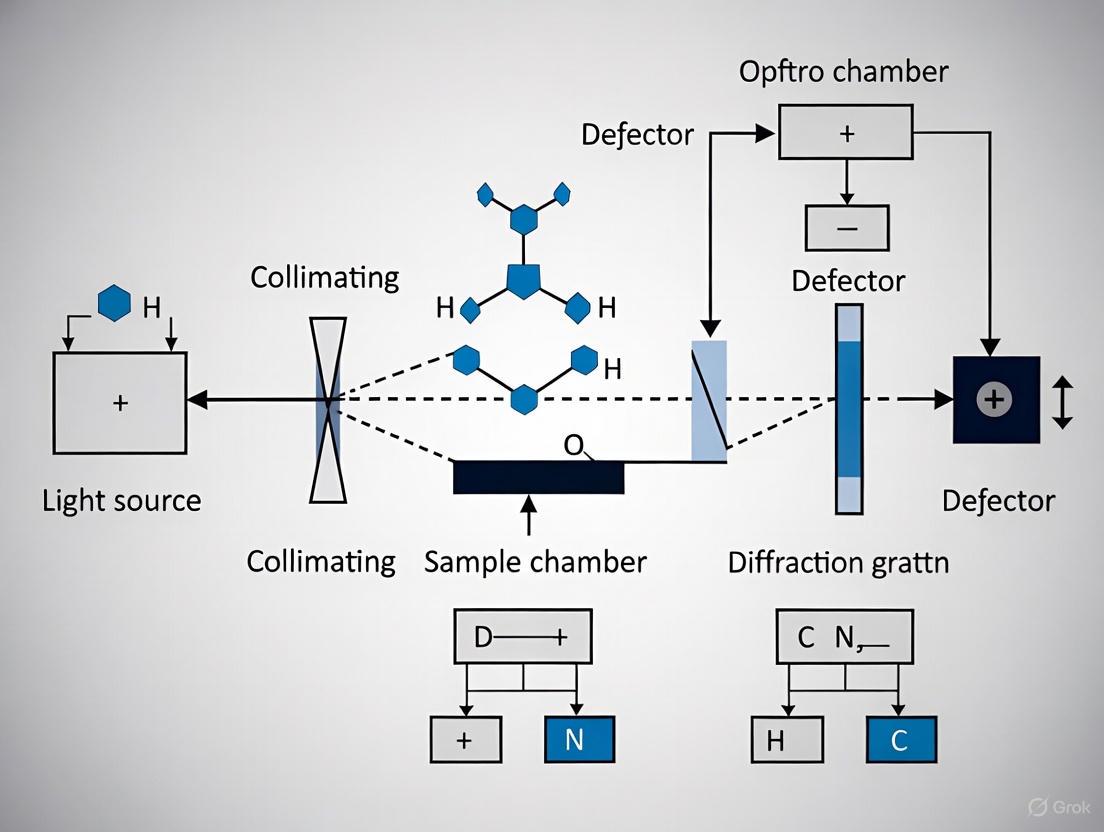
The optical path of a dispersive spectrometer consists of several key components, each serving a specific function in the process of generating and analyzing spectral data. The following diagram illustrates the fundamental layout and component relationships in a classic dispersive spectrometer.

The fundamental components of a dispersive spectrometer optical path include:

• Light Source: Provides illumination across the spectral range of interest. For Raman spectroscopy, semiconductor lasers at specific wavelengths (e.g., 785 nm) are commonly used [4] [1].
• Input Slit: Defines the entrance aperture and affects both optical resolution and signal intensity. A narrower slit provides better resolution but reduces throughput [4] [1].
• Collimation Mirror: Converts the divergent beam from the slit into a parallel (collimated) beam, ensuring uniform illumination of the dispersive element.
• Diffraction Grating: Angularly disperses different wavelengths of light according to the grating equation: mλ = d(sinα + sinβ), where m is the diffraction order, λ is wavelength, d is the groove spacing, and α and β are the angles of incidence and diffraction, respectively [4].
• Focus Mirror: Focuses the dispersed wavelengths onto different positions of the detector array.
• Detector Array: Captures the intensity of light at different wavelengths simultaneously. Common detectors include CCD and CMOS arrays with specific spectral response characteristics [4].

Design Trade-offs and Performance Parameters

The design of a spectrometer optical path involves balancing several competing performance parameters. The key relationships governing this balance are quantified in the following table.

Table 1: Key Performance Relationships in Spectrometer Optical Path Design

Parameter	Mathematical Relationship	Design Impact	Application Consideration
Spectral Resolution	Δλ = λ²/(2Δz) for Gaussian window (STFT) [5]	Shorter spatial window (Δz) improves spatial resolution but worsens spectral resolution	Higher resolution needed for distinguishing closely spaced spectral features
Focal Length	L_F ≈ L_D / [G · (λ₂ - λ₁) · cosβ] [4]	Higher groove density (G) or smaller detector (L_D) enables shorter focal length	Compact designs favor high groove density gratings and smaller detectors
Numerical Aperture	NA = sin(θ) where θ is half-angle of input cone	Higher NA increases light throughput but requires larger optical elements	Critical for weak signal applications like Raman spectroscopy
Optical Resolution	Δλ_FWHM ≈ λ/(G · w_beam) where w_beam is beam width on grating [4]	Wider illumination on grating improves resolution	Limited by physical size constraints of spectrometer

The focal length of the focusing mirror (L_F) is a primary determinant of overall spectrometer size. As shown in Figure 2 of the search results, the focal length can vary by nearly two orders of magnitude depending on the selected grating groove density and detector size [4]. For a compact Raman spectrometer covering 800-1100 nm, using a 1800 lines/mm grating with a ¼-inch detector enables a focal length of approximately 30 mm, resulting in a footprint as small as 30×30 mm [4].

The numerical aperture (NA) determines the light-gathering ability of the spectrometer. A higher NA collects more light from the sample, which is particularly important for weak signals like Raman scattering, but requires larger optical elements to accommodate the wider light cone, creating a trade-off between compactness and sensitivity [4]. For battery-operated portable instruments, this trade-off often favors designs that maximize throughput while maintaining reasonable size constraints.

Experimental Methods and Protocols

Raman Spectrometer Implementation Protocol

The implementation of an experimental Raman spectrometer follows a systematic methodology with specific protocols for component selection, assembly, and characterization:

• Light Source Selection and Characterization: Choose a laser diode with wavelength appropriate for the sample (e.g., 785 nm for reduced fluorescence in biological samples). Characterize the optical power output versus drive current using a power meter. The laser principle follows the equation: P_optical = η · (I - I_th), where P_optical is output power, η is slope efficiency, I is drive current, and I_th is threshold current [1].

• Optical Path Configuration: Connect the laser to a multimode optical probe using a matching sleeve. Incorporate a notch filter with the same wavelength as the pump laser to reject the elastically scattered Rayleigh light while transmitting the Raman-shifted signal. Precisely align the filter using micro-positioners [1].

• Spectrometer Core Setup: Configure the spectrometer with appropriate slit width (e.g., 25 μm), grating groove density (e.g., 600 lines/mm for general purpose), and detector array. Calculate the expected spectral range using the grating equation and verify the optical resolution based on slit width and diffraction limitations [1].

• Wavelength Calibration: Use a calibration source with known emission lines (e.g., argon lamp) to establish the relationship between detector pixel position and wavelength. Measure the full width at half maximum (FWHM) of narrow emission lines to determine experimental resolution [4] [1].

• System Performance Validation: Record Raman spectra of standard materials with known spectra (e.g., silicon) and compare with reference databases to verify correct spectral acquisition and resolution. The RRUFF database provides reference spectra for mineral validation [1].

The following workflow diagram illustrates the key stages in implementing and validating a Raman spectrometer system.

Spectroscopic OCT Analysis Protocol

Spectroscopic Optical Coherence Tomography (sOCT) requires specialized analysis methods to extract depth-resolved spectral information. The following protocol outlines the key steps for sOCT analysis using the Short-Time Fourier Transform (STFT) method, which has been identified as optimal for hemoglobin concentration and oxygen saturation quantification [5]:

• Data Acquisition: Acquire interferometric data either directly in the spatial domain (time-domain OCT) or through Fourier transformation of spectral domain data. Ensure proper sampling to satisfy the Nyquist criterion for the desired spectral range.

• Spatial Windowing: Apply a spatial window w(z, Δz) centered at depth z with width Δz to the interferometric signal i_D(z'). Gaussian windows are commonly used for their optimal time-frequency localization properties [5].

• Spectral Transformation: Compute the STFT using the equation: STFT(k,z;w) = ∫[-∞,∞] i_D(z') · w(z-z'; Δz) · e^(-ikz') dz' This generates a complex-valued spectrogram with depth and wavenumber axes [5].

• Spectral Analysis: Take the amplitude of the complex spectrogram to obtain the depth-resolved power spectrum. Analyze the spectral features at each depth to determine wavelength-dependent absorption and scattering properties.

• Chromophore Quantification: Fit the extracted absorption spectra to known chromophore extinction coefficients (e.g., oxy- and deoxyhemoglobin) using least-squares methods to determine concentration and oxygen saturation.

The performance of sOCT analysis methods can be quantitatively compared using the mean squared difference (χ²) between input and recovered absorption coefficient spectra, with particular attention to errors in derived hemoglobin concentration and oxygen saturation [5].

Data Analysis and Interpretation Methods

Spectrum Reconstruction Techniques

The reconstruction of spectra from detector signals involves solving a linear system that describes how the spectrometer responds to different wavelengths. The generic model for a spectrometer can be represented as: I_i = ∫ R_i(λ) T_i(λ) S(λ) dλ + η_i where I_i is the signal intensity on the i-th detector, R_i(λ) is the detector responsivity, T_i(λ) is the optical transmittance for that detector path, S(λ) is the input power spectral density, and η_i is the measurement noise [6].

Discretizing this equation leads to the matrix formulation: y = Gs + η where y is the measurement vector, G is the system matrix representing the combined optical and detector response, s is the discretized spectrum vector, and η is the noise vector [6]. The spectrum reconstruction problem involves inverting this relationship to estimate s given the measurements y.

For well-conditioned square system matrices, direct inversion ŝ = G⁻¹y is possible. However, most practical systems require regularization to handle noise and ill-conditioning. Tikhonov regularization (ridge regression) solves: ŝ = argmin ‖Gs - y‖₂² + α‖s‖₂² where α ≥ 0 is a regularization parameter that controls the trade-off between data fidelity and solution smoothness [6]. This approach is particularly valuable for miniaturized spectrometers and integrated photonic spectrometers where the system matrix may be inherently ill-conditioned due to size constraints.

Advanced Time-Frequency Analysis

In spectroscopic OCT and related techniques, advanced time-frequency analysis methods enable the extraction of depth-resolved spectral information. The key methods include:

• Short-Time Fourier Transform (STFT): Applies a fixed window to the signal before Fourier transformation, providing constant time-frequency resolution throughout the frequency spectrum. The spatial resolution Δz and spectral resolution Δk are related by Δk = 1/(2Δz) for a Gaussian window [5].

• Wavelet Transform: Uses variable window sizes adapted to frequency, providing better spatial resolution at high frequencies and better spectral resolution at low frequencies. This method maintains constant relative bandwidth across the spectrum [5].

• Wigner-Ville Distribution: A bilinear distribution that provides high resolution in both time and frequency domains but suffers from interference terms between signal components, making interpretation challenging [5].

• Dual Window Method: Combines two STFTs with different window sizes to partially overcome the resolution trade-off inherent in single-window methods [5].

For the specific application of quantifying hemoglobin concentration and oxygen saturation, studies have concluded that STFT provides the optimal balance of spectral/spatial resolution and accurate spectral recovery, minimizing errors in the derived physiological parameters [5].

Research Toolkit: Essential Components and Reagents

Table 2: Research Reagent Solutions for Spectrometer Development and Application

Component/Reagent	Function	Example Specifications	Application Notes
NIR Diode Laser	Excitation source for Raman spectroscopy	785 nm, 0-100 mW adjustable power (Thorlabs LP785SF-100) [1]	Reduced fluorescence in biological samples; power adjustable for different sample types
Notch Filter	Rejects Rayleigh scattered laser light	Center wavelength matching laser (e.g., 785 nm) [1]	Critical for detecting weak Raman signals; requires precise positioning
Diffraction Grating	Disperses light into spectral components	600-1800 lines/mm, dependent on application [4]	Higher groove density enables more compact designs; efficiency varies with wavelength
CCD/CMOS Detector	Captures dispersed spectrum	1024-3648 pixels, back-thinned for enhanced NIR response [4] [1]	Cooling reduces dark noise but increases power consumption; pixel size affects resolution
Calibration Source	Wavelength scale calibration	Argon lamp with known emission lines [4] or white-light tungsten lamp [1]	Essential for accurate wavelength assignment; should be traceable to standards
Optical Fibers	Light delivery and collection	Multimode fibers for higher light throughput [1]	Enable flexible sample presentation; numerical aperture affects light collection efficiency
85Rb Vapor Cell	Quantum light generation	Dense vapor for four-wave mixing [3]	Used in quantum spectroscopy for generating squeezed light with reduced noise
Nonlinear Crystals	Wavelength conversion and squeezing	χ⁽²⁾ materials for optical parametric amplification [3]	Enable frequency conversion and generation of non-classical light states

The selection of appropriate components depends on the specific spectroscopic technique and application requirements. For medical diagnostics using Raman spectroscopy, the optimization of these components enables the development of systems capable of in vivo, real-time "optical biopsy" without the need for sample preparation or destructive processing [1]. For advanced research involving quantum-enhanced measurements, elements like 85Rb vapor cells and nonlinear crystals enable the generation of squeezed light that can surpass the standard quantum limit, providing superior measurement precision [3].

The continuing miniaturization of spectroscopic components, including the development of integrated photonic spectrometers, promises to further expand applications in point-of-care diagnostics, environmental monitoring, and pharmaceutical development while reducing the size, weight, power, and cost of analytical systems [6].

This technical guide provides an in-depth analysis of the core components that constitute a modern optical spectrometer, tracing the optical path from illumination to detection. Aimed at researchers and scientists in drug development and related fields, this whitepaper synthesizes current instrumentation principles to support foundational research in spectrometer optical path design. The performance of a spectrometer is governed by the intricate interplay between its constituent parts, where optimization of one component often involves trade-offs with others. Understanding these relationships is crucial for selecting appropriate instrumentation for specific applications, from routine concentration assays to advanced research in photochemistry and biopharmaceutical analysis.

An optical spectrometer is an instrument used to measure the intensity of light as a function of its wavelength or frequency [7]. It is a foundational tool in scientific research, enabling the qualitative and quantitative analysis of materials by examining their interaction with electromagnetic radiation. In pharmaceutical and biotech research, spectrometry is indispensable for tasks ranging from characterizing protein stability and vaccine components to monitoring chemical reactions and ensuring product purity [2].

The fundamental operating principle of any spectrometer involves separating incoming polychromatic light into its constituent wavelengths and quantitatively measuring the intensity of each spectral component [8]. This process occurs within a structured optical path, where each component plays a critical role in defining the instrument's final performance characteristics, including its spectral range, resolution, sensitivity, and signal-to-noise ratio. The following sections dissect these key components in detail, from the entrance slit to the detector.

The Optical Path: Component Breakdown

Entrance Slit

The entrance slit is the gateway through which light enters the spectrometer, serving as the effective object that the rest of the optical system images onto the detector. Its primary functions are to control the amount of light entering the system and to define the theoretical resolution limit of the instrument [9].

Function and Trade-offs: The width of the entrance slit is one of the main parameters determining the resolution of the spectrometer and the amount of light that can enter for processing [9]. A narrower slit provides higher spectral resolution by more strictly limiting the angles of light entering the optical system, which reduces optical aberrations and creates sharper images on the detector. However, this comes at the cost of reduced optical throughput, which can increase the measurement time required to acquire a signal with adequate signal-to-noise characteristics. Conversely, a wider slit maximizes light intake, beneficial for low-light applications, but decreases spectral resolution by allowing a broader range of wavelengths to reach each detector pixel [9] [8].

Technical Specifications: Slits are available in a wide range of widths, typically from 5 µm up to 800 µm, with heights generally standardized between 1 mm and 2 mm [9]. Due to its critical alignment requirements, the slit is often permanently mounted within the spectrometer, making the initial choice of slit width a significant decision that balances resolution and throughput needs for the intended application [9].

Collimating and Focusing Optics

Once light passes through the entrance slit, it diverges and must be collimated before reaching the dispersive element. This is typically accomplished by a collimating mirror, which creates a beam of parallel rays. After dispersion, a focusing mirror directs the separated wavelengths onto the detector plane.

Optical Configurations: The most common configuration for compact spectrometers is the Czerny-Turner design, which uses two concave mirrors—one for collimating and one for focusing [7] [10]. This design is favored for its flexibility, relatively low cost, and ability to produce a flat focal plane ideal for array detectors. Variations include the Crossed Czerny-Turner, which offers a more compact layout but may introduce more optical aberrations, and the Unfolded Czerny-Turner (or "W" configuration), which incorporates beam blocks to reduce stray light and improve the signal-to-noise ratio, particularly beneficial for low-light applications like Raman spectroscopy [7].

An alternative design is the concave holographic spectrograph, where a single concave grating performs both the dispersion and focusing functions, reducing the number of optical components and associated stray light [7].

Dispersive Element

The heart of the spectrometer is the dispersive element, which spatially separates light by its wavelength. While prisms can be used, diffraction gratings are the most common dispersive element in modern instruments [8].

Operating Principle: A diffraction grating operates on the principle of diffraction and interference. It consists of a surface with a large number of parallel, equally spaced grooves. The fundamental grating equation that governs the dispersion is: [ d\sin(Θ) = mλ ] where ( d ) is the grating spacing, ( Θ ) is the diffraction angle, ( m ) is the diffraction order, and ( λ ) is the wavelength of light [7] [8]. This relationship shows how different wavelengths are diffracted at different angles.

Grating Types and Selection:

• Ruled Gratings: Manufactured by physically etching grooves onto a reflective substrate with a diamond tool. They offer flexibility and can operate across a wide wavelength range (50 nm to 50 µm) with groove densities from 50 to 3600 grooves/mm [7].
• Holographic Gratings: Produced optically using laser-created interference patterns, resulting in more consistent groove spacing and form. This leads to superior performance in terms of lower stray light and higher fidelity, but they are typically optimized for a more fixed spectral range [7] [10].

The choice of grating involves a critical trade-off. Gratings with higher groove density (e.g., 1200-3600 lines/mm) provide higher spectral resolution but cover a narrower wavelength range. Those with lower groove density (e.g., 300-600 lines/mm) cover a broader range but with lower resolution [10].

Detector

The detector translates the optical signal at the focal plane into an electrical signal for quantitative analysis. It is the final critical component in the optical path. Detectors are broadly classified as single-channel or multichannel detectors [11].

Detector Technologies:

• Silicon CCD (Charge-Coupled Device): The most common detector for UV-Vis applications (∼200-1100 nm). Scientific-grade CCDs offer high dynamic range and uniform pixel response. They can be front-illuminated (often with a phosphor coating for UV enhancement) or back-thinned for higher quantum efficiency [11] [10].
• CMOS (Complementary Metal-Oxide-Semiconductor): Similar to CCDs but often favored for high-speed applications due to faster readout capabilities [10].
• InGaAs (Indium Gallium Arsenide): Used for near-infrared (NIR) measurements, typically from 900-2500 nm, bridging the gap where silicon becomes transparent [11] [10].
• Photomultiplier Tube (PMT): A classic single-channel detector known for high gain and excellent sensitivity for low-light-level detection, though it requires scanning to build a full spectrum [11].

Performance Enhancement: To reduce electronic noise (dark current), detectors, especially CCDs used in sensitive applications, are often thermoelectrically cooled [11] [8]. For instance, specialized spectrometers for Raman spectroscopy feature cooled detectors to maintain signal integrity during long integration times [10].

Table 1: Key Spectrometer Components and Their Performance Characteristics

Component	Key Function	Design Trade-offs	Common Types/Specifications
Entrance Slit	Controls light input and resolution [9]	Narrow width → Higher resolution, Lower throughput [9] [8]	Width: 5-800 µm; Height: 1-2 mm [9]
Optics	Collimates and focuses light	Complex design → Lower stray light vs. size/complexity	Czerny-Turner, Concave Holographic [7]
Diffraction Grating	Spatially separates light by wavelength [7] [8]	High groove density → Higher resolution, Narrower range [10]	Ruled, Holographic; 300-3600 lines/mm [7] [10]
Detector	Converts light to electrical signal [11]	High sensitivity vs. speed vs. cost vs. spectral range	CCD, CMOS, InGaAs, PMT; Cooled/Uncooled [11] [10]

The Integrated System: From Light to Data

The components described above function as an integrated system to convert incoming light into a usable spectrum. The process begins when light from a sample or source is delivered to the entrance slit, often via fiber optics [10]. The slit defines the source geometry, and the collimating mirror directs a parallel beam onto the grating. The grating then angularly disperses the light, sending different wavelengths in different directions. The focusing mirror converges these diverging beams, creating a series of images of the entrance slit—each at a different wavelength—across the focal plane where the detector is located [12].

In a multichannel spectrometer with a fixed grating, each pixel on the linear detector array corresponds to a specific narrow band of wavelengths [10]. The intensity recorded at each pixel is digitized and processed by software to generate a plot of intensity versus wavelength—the final spectrum. The calibration that maps pixel position to wavelength is a critical step, derived from the grating equation and verified using light sources with known emission lines [12].

Experimental Protocols for System Characterization

To ensure accurate and reliable data, characterizing the performance of a spectrometer system is essential. The following protocols outline key experiments.

Protocol for Spectral Resolution and Bandpass Measurement

Objective: To determine the minimum resolvable wavelength difference of the spectrometer system.

• Setup: Illuminate the entrance slit with a low-pressure spectral calibration lamp (e.g., Mercury-Argon) that emits sharp, known atomic emission lines.
• Data Acquisition: Acquire a spectrum of the calibration lamp with the spectrometer. Use integration times that avoid detector saturation.
• Analysis: Identify a well-isolated, narrow emission line in the captured spectrum. Measure the Full Width at Half Maximum (FWHM) of this peak. The FWHM (in nanometers) is the instrumental bandpass, a direct measure of its resolution capability [10].

Protocol for Signal-to-Noise (S/N) Optimization

Objective: To maximize the S/N ratio for a given measurement, a critical parameter for detecting small absorbance differences (chemometric sensitivity) [10].

• Setup: Connect a stable light source (e.g., tungsten-halogen) to the spectrometer via fiber optics.
• Baseline Measurement: Block the light source and acquire a "dark" spectrum with the same integration time as the test measurement. This captures the detector's noise floor.
• Signal Measurement: Acquire a spectrum of the light source.
• Optimization: The S/N ratio is proportional to the square root of both the signal intensity and the number of spectral averages. To optimize:
  • Increase Integration Time: Lengthen the exposure until just before saturation occurs.
  • Software Averaging: Acquire and average multiple spectra. The S/N improves with the square root of the number of averages (e.g., 4 averages improve S/N by 2x) [10].
  • Slit Width: If adjustable, a wider slit will increase signal but decrease resolution.

Research Reagent Solutions: Essential Materials

The following table details key components and materials essential for configuring and operating a spectrometer system for research applications.

Table 2: Essential Research Reagents and Materials for Spectrometry

Item	Function/Description	Application Example
Spectral Calibration Lamp	A light source with known, sharp emission lines (e.g., Hg, Ne, Ar).	Wavelength accuracy verification and system calibration [5].
Stable Broadband Light Source	A source emitting continuous spectrum (e.g., Tungsten-Halogen, Deuterium).	As a reference for absorbance measurements and system alignment.
NIST-Traceable Standards	Filters or materials with certified optical properties.	Validating photometric accuracy (e.g., absorbance, transmittance).
Fiber Optic Probes	Flexible light guides for remote sampling.	Measuring samples in reactors, living tissues, or harsh environments [10].
Integration Sphere	A device producing a spatially uniform light source.	Measuring diffuse reflectance of scattering samples.
Ultrapure Water System	Provides water free of chemical and particulate contaminants.	Sample preparation, dilution, and cleaning of cuvettes to prevent stray light [2].

Visualizing Spectrometer Workflows

Optical Path and Signal Processing

The following diagram illustrates the physical path of light through a Czerny-Turner spectrometer and the subsequent electronic signal processing.

Resolution vs. Throughput Trade-off

This diagram visualizes the critical engineering trade-off governed by the entrance slit width.

The performance of a modern optical spectrometer is a direct consequence of the careful selection and integration of its core components: the entrance slit, collimating and focusing optics, diffraction grating, and detector. As evidenced by the latest instrumentation reviews, the field continues to evolve with trends toward miniaturization, higher sensitivity, and greater application-specific customization, such as systems dedicated to biopharmaceutical analysis [2]. A deep understanding of the optical path and the inherent trade-offs between resolution, sensitivity, and speed empowers researchers to make informed decisions when selecting or configuring a spectrometer. This foundational knowledge is crucial for leveraging this powerful analytical technology to its fullest potential in drug development and scientific research.

Spectrometers are indispensable instruments across numerous scientific and industrial fields, from chemical analysis and biomedical research to environmental monitoring and pharmaceutical development. Their fundamental purpose is to dissect light into its constituent wavelengths, providing a fingerprint of the matter with which it has interacted. The optical geometry at the heart of any spectrometer is the primary determinant of its performance characteristics, including spectral range, resolution, signal-to-noise ratio, and physical footprint.

This whitepaper provides an in-depth technical guide to three foundational spectrometer configurations: the Czerny-Turner, Fourier Transform Infrared (FT-IR), and Littrow geometries. Understanding the principles, advantages, and limitations of these classical optical paths is crucial for researchers, scientists, and drug development professionals seeking to select, optimize, or develop spectroscopic methods for their specific applications. The content is framed within the broader context of spectrometer optical path component research, emphasizing the design trade-offs inherent in achieving desired analytical performance.

Core Principles and Optical Geometries

Czerny-Turner Configuration

The Czerny-Turner (C-T) configuration is a workhorse in spectroscopy, renowned for its excellent performance over a broad spectral range [13]. It is a prime example of a design following the fixed geometry convention in the grating equation, denoted as Φ = α + β, where Φ is the fixed deviation angle and α and β are the angles of incidence and diffraction, respectively [13].

As illustrated in Diagram 1, a typical C-T system comprises an entrance slit, a spherical collimating mirror, a planar diffraction grating, a spherical focusing mirror, and a detector array [13] [14]. Light enters through the slit and is collimated by the first mirror. This collimated beam strikes the diffraction grating, where it is separated into its constituent wavelengths. The diffracted light is then focused by the second spherical mirror onto the detector array [13]. The two-mirror design allows for precise control of optical aberrations, leading to high-quality spectral data.

A significant challenge in C-T designs is managing off-axis aberrations such as coma, astigmatism, and field curvature, which worsen as the off-axis angle increases [14]. To meet the demand for portable, high-performance spectrometers, advanced aberration correction methods have been developed. These include using the Shafer equation to correct coma at a central wavelength, optimizing the grating position to correct field curvature, and introducing tailored optical elements like tilt and wedge cylindrical lenses to eliminate astigmatism across the entire spectral band [14].

FT-IR Configuration

Fourier Transform Infrared (FT-IR) spectroscopy operates on a fundamentally different principle than dispersive spectrometers. Instead of spatially separating wavelengths, it uses an interferometer to encode all spectral information simultaneously into an interference pattern, which is then converted into a spectrum using a Fourier Transform [15] [16].

The most common interferometer is the Michelson type, consisting of a beam splitter, a fixed mirror, and a moving mirror [16]. Broadband IR light from the source is split into two beams. These beams are reflected from the fixed and moving mirrors, respectively, and recombine at the beam splitter, creating an interference pattern known as an interferogram that is directed to the detector [15] [16]. The central peak of this interferogram, the centerburst, occurs at the Zero Path Difference (ZPD), the point where the optical paths of the two beams are equal and all wavelengths interfere constructively [16]. The spectral resolution of an FT-IR is inversely proportional to the maximum Optical Path Difference (OPD) achieved by the moving mirror [16].

Modern FT-IR designs often enhance stability and performance. For instance, some systems employ a compact, highly stable double-moving mirror swing interferometer with cube corner reflectors to generate OPD. Cube corner reflectors reduce alignment sensitivity and allow for a larger OPD in a smaller physical space, making the interferometer more robust and compact [17].

FT-IR spectrometers hold several inherent advantages over dispersive instruments, known as the Felgett (multiplex) advantage, Jacquinot (throughput) advantage, and Connes' advantage [15]. These contribute to higher signal-to-noise ratios, faster acquisition times, better spectral resolution, and superior wavelength accuracy [15] [16].

Littrow Configuration

The Littrow configuration is a specific alignment for optical systems containing a reflective grating wherein the grating is oriented so that the diffracted light for a particular order (often the first order) travels back along the direction of the incident beam [18]. This configuration is useful in applications such as laser resonators, where the grating can act as one of the cavity mirrors, and in certain monochromators and spectrometers [18].

In the Littrow condition, the angles of incidence and diffraction are approximately equal (α ≈ -β), meaning the light is diffracted directly back on itself [13] [18]. This leads to a very straight, compact optical path. A common spectrometer design that utilizes the Littrow condition is the Lens Grating Lens (LGL) configuration [13]. In an LGL system, light passes through a collimation lens, a transmission diffraction grating, and a focusing lens before reaching the detector. This transmission-based design is typically more compact and cost-effective than mirror-based systems like the C-T, though it may offer less control over certain aberrations [13].

Table 1: Key Characteristics of Classical Spectrometer Geometries

Feature	Czerny-Turner	FT-IR	Littrow (LGL Example)
Dispersion Method	Diffraction Grating (Reflection)	Interferometry (Michelson)	Diffraction Grating (Transmission)
Typical Components	Entrance slit, two spherical mirrors, planar grating	Beam splitter, fixed & moving mirrors, detector	Entrance slit, two lenses, transmission grating
Optical Path	Folded (fixed deviation angle)	Interferometric	Straight, compact
Primary Advantage	Excellent aberration control, broad range	High speed, SNR, and throughput (Multiplex & Throughput advantages)	Compact size, simplicity
Common Spectral Range	UV-VIS-NIR	NIR-FIR (0.77 - 200 µm reported) [17]	VIS-NIR
Reported Resolution	0.01 nm demonstrated [14]	0.25 cm⁻¹ demonstrated [17]	Varies with miniaturization

Comparative Performance and Advanced Design

Quantitative Performance Metrics

The selection of an optical geometry directly impacts critical performance parameters. The following table summarizes key metrics as demonstrated in recent research.

Table 2: Reported Performance Metrics from Recent Spectrometer Designs

Configuration	Spectral Range	Resolution	Signal-to-Noise Ratio (SNR)	Key Innovation
Ultra-Wide-Band FT-IR [17]	0.770 – 200 µm (50 - 13,000 cm⁻¹)	0.25 cm⁻¹	> 50,000:1	Double-moving mirror swing interferometer; switchable sources/detectors
Aberration-Corrected Crossed C-T [14]	440 – 640 nm	0.2 nm (@546.07 nm)	Not Specified	Tilt/wedge cylindrical lens for astigmatism correction; sine-constrained calibration
Portable Grating Spectrometer [19]	3800 cm⁻¹ range	1.4 cm⁻¹	Low noise (no cooling required)	Based on fast F0.95/50 mm camera lens; volume < 2 L
Planar Waveguide C-T [20]	450 – 750 nm	< 4 nm	Optimized via sagittal plane design	Hollow planar waveguide for miniaturization; separate tangential/sagittal design

Advanced Design Considerations and Aberration Correction

Achieving high performance requires careful attention to optical design and the correction of aberrations. For Czerny-Turner systems, a key advancement is the move beyond simple spot diagram evaluation to criteria that balance luminous flux and aberration (LFAB), control the variation of the Airy disk at imaging points (ADVI), and ensure optical-detector resolution matching (ORDM) [21]. This holistic approach allows designers to increase the numerical aperture at the slit (e.g., to 0.11) to collect more light for weak signal detection while still maintaining controlled aberrations and a uniform performance across the spectral band [21].

For miniaturization, the hollow planar waveguide spectrometer (HPWS) based on the C-T structure represents a significant innovation. In this design, the light beam travels between two parallel mirrors, folding the optical path. The design is separated into the tangential plane (affecting resolution) and the sagittal plane (affecting energy throughput). The height of the waveguide is a critical parameter, as it determines the number of reflections and thus the energy loss, requiring careful optimization to ensure the detector receives sufficient optical flux [20].

In FT-IR systems, the design of the infrared light source and its collimation is crucial. One design uses a secondary imaging scheme with an ellipsoidal reflector to image the radiation source onto a variable diaphragm, which is then collimated by an off-axis parabolic mirror. This scheme tightly controls the beam divergence angle (e.g., to 4 mrad), which is essential for achieving high spectral resolution (e.g., 0.25 cm⁻¹) [17].

Experimental Protocols and Methodologies

Protocol for Aberration Correction in a Czerny-Turner Spectrometer

This protocol is adapted from methods used to achieve high resolution and imaging quality in portable spectrometers [14].

Objective: To correct for coma, astigmatism, and field curvature in a crossed Czerny-Turner spectrometer to achieve a target resolution of 0.2 nm or better.

Materials and Reagents:

• Optical Bench or Breadboard: A stable, vibration-damped platform.
• Spectrometer Components: Entrance slit, spherical collimating mirror, planar diffraction grating (e.g., 1800 grooves/mm), spherical focusing mirror, and a CCD detector.
• Aberration Correction Element: A cylindrical lens with adjustable tilt and wedge angles.
• Light Sources for Calibration: Mercury-argon (Hg-Ar) lamp or other sources with known, sharp emission lines (e.g., 546.07 nm).
• Alignment Tools: He-Ne laser, pinholes, and power meter.

Procedure:

• Initial Assembly: Mount the optical components (slit, collimating mirror, grating, focusing mirror) in the crossed C-T layout according to the designed angles and distances.
• Coma Correction: Adjust the angles of the collimating and focusing mirrors to satisfy the Shafer coma-free condition for the central wavelength [14].
• Field Curvature Correction: Translate the diffraction grating along the optical axis to find the position that minimizes field curvature on the detector plane.
• Astigmatism Correction: a. Insert the cylindrical lens between the focusing mirror and the detector. b. Systematically adjust both the tilt and wedge angles of the cylindrical lens while illuminating the system with a known spectral line. c. Iterate until the spot size on the detector is minimized and symmetric across the spectral range, indicating eliminated astigmatism.
• Wavelength Calibration: a. Illuminate the slit with the Hg-Ar calibration lamp. b. Record the positions of known spectral lines on the CCD. c. Establish the relationship between pixel position and wavelength using a sine-constrained least squares fitting algorithm, which has been shown to achieve accuracy of 0.01 nm [14].
• Validation: Measure the full width at half maximum (FWHM) of a narrow emission line (e.g., 546.07 nm) to confirm the spectral resolution meets the 0.2 nm target.

Protocol for Characterizing an Ultra-Wide-Band FT-IR Spectrometer

This protocol outlines the key steps for verifying the performance of a wide-band FT-IR system, based on a design covering from the visible to the far-infrared [17].

Objective: To verify the spectral range, resolution, and signal-to-noise ratio of an ultra-wide-band FT-IR spectrometer.

Materials and Reagents:

• FT-IR Spectrometer: Equipped with a double-moving mirror interferometer, and switchable sources (e.g., air-cooled SiC for MIR/FIR, halogen tungsten for NIR) and detectors.
• Beam Splitter(s): Optimized for different spectral regions (e.g., NIR, MIR, FIR).
• Nitrogen Purge System: To remove atmospheric water vapor and CO₂.
• Reference Materials: Polystyrene film, known gas cells (e.g., CO), and a mid-infrared linearity standard.
• Software: Capable of performing Fast Fourier Transform (FFT), apodization, and phase correction.

Procedure:

• System Configuration: a. Select the appropriate combination of light source, beam splitter, and detector for the initial target spectral band (e.g., MIR). b. Allow the system to warm up and purge the optical compartment with dry nitrogen for at least 30 minutes.
• Background Measurement: Collect a high-SNR background interferogram with no sample in the beam path. This will be used to ratio against sample measurements.
• Spectral Range Verification: a. For NIR Verification: Switch to the halogen lamp source and a corresponding detector. Acquire a spectrum of a known NIR-reflective material. b. For FIR Verification: Switch to the SiC source and a dedicated FIR detector. Acquire a spectrum of a polyethylene window or another FIR-transparent material. c. Confirm that the measured spectra show meaningful signal levels at the extremes of the claimed range (e.g., 0.77 µm and 200 µm) [17].
• Resolution Measurement: a. Introduce a gas cell containing a low-pressure gas with sharp, well-defined rotational-vibrational lines (e.g., CO) into the sample compartment. b. Acquire an interferogram with a long optical path difference (e.g., corresponding to a resolution of 0.25 cm⁻¹). c. Transform the interferogram and examine the FWHM of an isolated gas line. The resolution is the FWHM of this line in cm⁻¹.
• Signal-to-Noise Measurement: a. Using the standard polystyrene film, acquire a high-quality reference transmission spectrum. b. Collect a series of rapid, single-scan spectra of the same sample under identical conditions. c. At a specific wavelength where the polystyrene has a strong peak (e.g., 1600 cm⁻¹), calculate the RMS noise in a nearby region with no spectral features. The SNR is the peak height divided by the RMS noise. A ratio of 50,000:1 is achievable [17].

Essential Research Reagent Solutions

The following table details key components and materials essential for the development and operation of high-performance spectrometers, as referenced in the experimental protocols and literature.

Table 3: Key Research Reagent Solutions for Spectrometer Development

Item	Function / Application	Technical Notes
Holographic Reflection Grating	Dispersive element in C-T spectrometers; separates light by wavelength.	1800 g/mm used in aberration-corrected design; line density and blaze angle determine efficiency and range [14].
Air-Cooled Silicon Carbide (SiC) Source	High-intensity broadband infrared emitter for MIR/FIR regions.	Spectral range 50–9600 cm⁻¹; air-cooling offers lower cost/power consumption vs. water or Peltier cooling [17].
Halogen Tungsten Lamp	Bright, continuous light source for NIR and Visible regions.	Spectral range 3000–25,000 cm⁻¹; used as switchable source in wide-band FT-IR [17].
Gold-Coated Optics (Mirrors, Cube Corners)	High-reflectivity mirrors and retroreflectors for IR light.	Gold film reflectivity >90% across NIR, MIR, FIR; K9 glass is a common, low-cost substrate [17].
Mercury-Argon (Hg-Ar) Calibration Lamp	Wavelength standard for accurate calibration of dispersive spectrometers.	Provides multiple, narrow emission lines at known wavelengths across a broad spectrum [14].
Cylindrical Lens (with Tilt/Wedge Adjustment)	Active optical element for astigmatism correction in C-T systems.	Placed between focusing mirror and detector; tilt and wedge angles are optimized to eliminate astigmatic focus [14].
Internal Reflection Element (IRE)	Core component of Attenuated Total Reflectance (ATR) sampling in FT-IR.	Diamond, ZnSe, or Ge crystals enable direct analysis of solids/liquids with minimal sample prep [15].
Nitrogen Purge Gas	Inert gas for purging optical path to remove atmospheric absorbers.	Eliminates spectral interference from water vapor and CO₂, crucial for quantitative IR analysis [15].

Diagrammatic Representations

The Role of Optical Path Length in Resolution and Sensitivity

In spectrometer design and application, the optical path length is a fundamental parameter that directly influences two critical performance metrics: resolution and sensitivity. Resolution defines an instrument's ability to distinguish between closely spaced spectral features, while sensitivity determines its capacity to detect weak signals. Within the context of optical path components research, understanding the role of path length is essential for optimizing spectrometer configurations for specific applications, from drug development to material characterization. This technical guide explores the underlying principles, quantitative relationships, and practical methodologies for leveraging optical path length to achieve desired analytical performance, providing researchers and scientists with a framework for informed instrument selection and experimental design.

Fundamental Principles of Optical Path in Spectrometry

The optical path in a spectrometer is the route light travels from the source, through various optical components, to the detector [22]. Its design lays out how light is collected, collimated, dispersed, and finally focused onto the detection system. The optical path length, specifically, can refer to the physical distance light travels within the instrument or, in sample analysis, the distance light travels through the sample itself. Both interpretations have a profound impact on the quality of the spectral data obtained.

A core principle governing light behavior in these systems is Fermat's principle, which states that light travels the path of least time [22]. Engineers use this principle to predict how light bends through lenses and at interfaces, ensuring consistent performance across wavelengths. The manipulation of light along the optical path involves three key stages:

• Collimation: Converting diverging light from the entrance slit into a parallel beam for even interaction with dispersive elements [22].
• Dispersion: Using prisms or diffraction gratings to split collimated light into its constituent wavelengths [22].
• Focusing: Using lenses or mirrors to focus the dispersed spectrum onto the detector plane [22].

The careful alignment of each stage is crucial for maintaining sharp wavelength resolution. Misalignment can introduce aberrations, leading to overlapping peaks or blurred spectra [22].

Optical Path Length and Spectral Resolution

Spectral resolution (R) is formally defined as R = λ/Δλ, where λ is the wavelength and Δλ is the smallest resolvable wavelength difference [23]. The optical path length within the spectrometer's optical bench is a key determinant of resolution.

The Grating Equation and Resolving Power

The resolution in diffraction-based systems is governed by the grating equation [22] [4]: [ d(\sin \alpha + \sin \beta) = m\lambda ] where (d) is the grating period, (\alpha) is the angle of incidence, (\beta) is the diffraction angle, and (m) is the diffraction order. The resolving power of a grating is given by (R = mN), where (N) is the total number of grooves illuminated by the light beam [24]. A longer optical path, often associated with a longer focal length ((LF) in Figure 1), allows for a wider beam width ((w{beam})) to illuminate more grating grooves. Equation 3 from the research demonstrates how this beam width limits the theoretical resolution [4]: [ \Delta\lambda{FWHM} = \frac{\lambda}{w{beam} G m} ] This shows that a wider beam, enabled by a longer focal length, directly improves the spectral resolution.

Focal Length and Instrument Size

The focal length of the spectrometer's focusing mirror is a primary factor in its physical size and resolution. The relationship between focal length ((LF)), detector length ((LD)), grating groove density ((G)), and wavelength range ((\lambda2 – \lambda1)) is approximated by [4]: [ LF \approx \frac{LD}{(\lambda2 - \lambda1) G \cos \beta} ] This indicates that for a fixed wavelength range and detector, a higher groove density grating can achieve the same resolution with a shorter focal length, enabling more compact spectrometer designs [4]. Figure 2 illustrates the nearly two-order-of-magnitude difference in spectrometer size achievable through different combinations of detector size and grating density.

Optical Path Length and Sensitivity

Sensitivity describes a spectrometer's ability to detect weak signals. The relationship between optical path length and sensitivity is particularly critical in absorption spectroscopy of samples.

Path Length in Absorption Spectroscopy

According to the Beer-Lambert law, the absorbance (A) of a sample is directly proportional to the concentration (c) of the analyte and the optical path length (l) through the sample: (A = \epsilon c l), where (\epsilon) is the molar absorptivity. A longer path length increases the measured absorbance, thereby improving the sensitivity for detecting low-concentration analytes [25]. This is especially valuable in Near-Infrared (NIR) spectroscopy of aqueous solutions, where analyte absorption is weak compared to the strong absorption bands of water [25].

The Signal-to-Noise Ratio and Detection Limits

The ultimate limit of detection (LOD) for an analyte is governed by the signal-to-noise (S/N) ratio [25]. While a longer sample path length increases the analytical signal (absorbance), research shows its effect on the S/N ratio is complex and must be optimized. A study investigating the detection of potassium hydrogen phthalate (KHP) in water found that optical path length is a key factor affecting the S/N ratio and thus the LOD [25]. However, an excessively long path can lead to signal loss if the dynamic range of the detector is exceeded. Therefore, the optimal path length balances sufficient signal enhancement against potential noise amplification or signal loss.

Quantitative Relationships and Trade-offs

The interplay between resolution, sensitivity, and optical path involves inherent trade-offs that must be managed during spectrometer design and experimental configuration.

Table 1: Impact of Spectrometer Component Changes on Performance

Component	Parameter Change	Effect on Resolution	Effect on Sensitivity
Entrance Slit	Narrower Width	Increases [24] [23]	Decreases (less light) [24] [23]
Diffraction Grating	Higher Groove Density	Increases [24] [10]	Decreases (more light dispersion) [24]
Optical Bench Focal Length	Longer Focal Length	Increases [4]	Decreases (lower throughput)
Sample Path Length	Longer Path Length	No Direct Effect	Increases (for absorption) [25]

Table 2: Experimental Limit of Detection (LOD) for KHP at Different Path Lengths [25]

Path Length (mm)	Aperture Type	Co-added Scans	Approximate LOD (ppm)
1	BRM2065	128	~300
2	BRM2065	128	~200
5	BRM2065	128	~150
10	BRM2065	128	>500

The data in Table 2, derived from a study on KHP detection, demonstrates that an optimal path length exists. While increasing the path from 1 mm to 5 mm improved the LOD, further increasing it to 10 mm was detrimental, likely due to excessive absorption by the solvent leading to a poor S/N ratio [25].

Experimental Protocols for Path Length Optimization

The following detailed methodology, adapted from a published study, provides a framework for empirically determining the optimal optical path length for a given application [25].

Determination of Optimal Sample Path Length for Aqueous Solutions

6.1.1 Research Objective: To determine the optimal optical path length that minimizes the Limit of Detection (LOD) for a specific analyte in an aqueous solution using transmission NIR spectroscopy and Partial Least Squares (PLS) calibration.

6.1.2 Materials and Reagents:

• Analyte: Potassium Hydrogen Phthalate (KHP).
• Solvent: Purified water.
• Stock Solution: 10,000 ppm KHP in purified water.
• Sample Set: 38 samples spanning 1 to 10,000 ppm, prepared via serial dilution from the stock solution.
• Cuvettes: Rectangular quartz cells with precisely defined path lengths (e.g., 1, 2, 5, and 10 mm).
• Spectrometer: FT-NIR spectrometer (e.g., Bruker Matrix-F) equipped with a fiber optic cable attachment and a TE-InGaAs detector.
• Software: For spectral acquisition (e.g., OPUS) and multivariate analysis (e.g., MATLAB).

6.1.3 Procedure:

• System Setup: Configure the FT-NIR spectrometer with a resolution of 8 cm⁻¹. Connect the fiber optic cable and install the temperature-controlled cuvette holder, setting it to 30.0 ± 0.1 °C.
• Baseline Collection: For each path length being tested, collect a reference spectrum using the corresponding empty quartz cell or a cell filled with purified water.
• Spectral Acquisition: For each KHP concentration and at each path length (e.g., 1, 2, 5, 10 mm): a. Place the sample in the temperature-controlled cuvette holder. b. Acquire transmission spectra over the relevant NIR range (e.g., 6300–5800 cm⁻¹, a spectral window between strong water absorptions). c. Collect multiple replicate spectra (e.g., 3 replicates). d. Repeat the measurements under different conditions of co-added scan times (e.g., 8, 16, 32, 64, 128) and aperture size to vary light intensity.
• Data Pre-processing: Apply necessary spectral pre-treatments to the absorbance data. The study compared no pre-treatment, linear baseline correction, Multiplicative Scattering Correction (MSC), and 2nd derivative (Savitzky-Golay) methods [25].
• Multivariate Calibration: Develop a PLS regression model for each path length condition, using the spectral data in the 6300–5800 cm⁻¹ range to predict KHP concentration. Use a method like leave-one-out cross-validation to determine the optimal number of latent variables and avoid overfitting [25].
• LOD Calculation: Calculate the LOD for each experimental condition according to IUPAC-consistent methods for PLS calibration, which account for types I and II errors and uncertainties in the slope and intercept of the calibration model [25].
• Optimal Path Identification: Compare the calculated LOD values across all path lengths. The path length yielding the lowest LOD represents the optimal compromise between signal enhancement and noise for that specific analyte-solvent system.

The Scientist's Toolkit: Essential Research Reagents and Materials

Table 3: Key Materials and Reagents for Spectroscopic Path Length Experiments

Item	Function / Rationale
Potassium Hydrogen Phthalate (KHP)	A common standard analyte for validating methods in aqueous solution; used for its well-defined C-H overtone bands in the NIR [25].
Precision Quartz Cuvettes	Provide a range of exact optical path lengths (e.g., 1, 2, 5, 10 mm) for transmission measurements; quartz is transparent in UV-Vis-NIR ranges.
FT-NIR Spectrometer	Enables high-throughput, high-signal-to-noise spectral acquisition across a broad NIR range, suitable for detecting weak overtone and combination bands [25].
TE-InGaAs Detector	Offers high sensitivity in the NIR region (e.g., 800-2500 nm), which is essential for detecting weak signals from aqueous solutions [25].
Partial Least Squares (PLS) Software	Multivariate analysis tool essential for extracting quantitative analyte information from complex, overlapping spectra typical of NIR data [25].

Visualization of Concepts and Workflows

The following diagrams illustrate the core relationships and experimental process discussed in this guide.

Diagram 1: Optical Path Length Relationships. This diagram shows how various design parameters influence optical path length and how path length, in turn, differentially affects resolution and sensitivity, creating a fundamental engineering trade-off.

Diagram 2: Path Length Optimization Workflow. This flowchart outlines the experimental protocol for empirically determining the optical path length that provides the lowest Limit of Detection for a specific analytical application.

The optical path length is a pivotal parameter in spectrometer design and operation, exerting a direct and often competing influence on resolution and sensitivity. A longer path within the optical bench enhances resolution by enabling finer wavelength discrimination at the detector, while a longer path through a sample boosts sensitivity for absorption measurements. However, these benefits are subject to practical constraints and trade-offs, necessitating a careful balance tailored to the specific analytical goal. As demonstrated in experimental research, an optimal path length exists that minimizes the detection limit, beyond which performance degrades. For researchers and scientists, a deep understanding of these principles is not merely academic but is an essential component of designing robust experiments, selecting appropriate instrumentation, and pushing the boundaries of what is detectable in fields ranging from pharmaceutical development to environmental monitoring.

The paraboloid of revolution crystal spectrometer represents a significant advancement in high-resolution X-ray spectroscopy, particularly for diagnostic precision in demanding fields such as inertial confinement fusion (ICF) research [26]. This innovative design simultaneously addresses three critical challenges in spectroscopic instrumentation: achieving high spectral resolution, maintaining high photon collection efficiency, and ensuring strict equal optical path conditions across a broad operational energy range [26] [27]. The fundamental operating principle leverages a curved crystal geometry configured to a paraboloid of revolution surface, which effectively suppresses spherical aberrations and ensures that all diffracted rays from the source to the detector traverse identical path lengths [26]. This equal-path property is crucial for minimizing phase differences and intensity attenuation, thereby enhancing spectral fidelity and imaging clarity [26]. For researchers and drug development professionals, understanding this technology is essential for pushing the boundaries of analytical capabilities in material characterization and elemental analysis.

Theoretical Foundation and Operating Principle

Fundamental Optical Geometry

The optical configuration of the paraboloid of revolution spectrometer is built upon a specific geometrical relationship between the X-ray source, the curved crystal, and the detector plane, as shown in the diagram below:

Figure 1: Optical geometry of the paraboloid of revolution spectrometer showing the equal-path relationship between source, crystal, and detector.

In this configuration, the X-ray source (S) is positioned at the focus of the parabolic crystal surface [26]. Incident rays from S undergo diffraction at point C on the crystal before reaching detection point P. The unique property of this arrangement is that every point on the crystal surface maintains an equal distance to both the directrix (a fixed reference line) and the X-ray source, establishing the fundamental equal optical path condition expressed mathematically as |SC| + |CP| = D + p, where D is the source-detector separation distance and p is the parabolic parameter [26].

Bragg Diffraction and Sagittal Focusing

The wavelength dispersion in this spectrometer follows Bragg's diffraction law, which governs X-ray interaction with crystalline materials [26]. The fundamental relationship is expressed as:

nλ = 2d sin θ

Where n is the diffraction order (typically n=1 for first-order diffraction), λ is the X-ray wavelength, d is the crystal interplanar spacing, and θ is the angle between the incident X-rays and the crystal plane [26]. For X-ray energy E, this relationship becomes E = hc/(2d sin θ), where h is Planck's constant and c is the speed of light [26].

To enhance photon collection efficiency without compromising resolution, the design incorporates sagittal focusing in the direction perpendicular to the dispersion plane [26]. This is achieved by constructing the crystal as a paraboloid of revolution rather than a simple parabolic curve. In the sagittal direction, an arc is constructed where all points share the same Bragg angle, ensuring that incident rays from the source diffracted at any point on this arc converge precisely at the detection point P [26]. This sagittal focusing mechanism enables simultaneous high resolution and high photon collection efficiency, even for relatively large source sizes.

Performance Specifications and Quantitative Data

The paraboloid of revolution spectrometer achieves remarkable performance characteristics, as verified through both simulation and experimental validation. The table below summarizes key performance metrics across different evaluation methods:

Table 1: Performance Specifications of Paraboloid of Revolution Spectrometer

Performance Parameter	Simulation Results	Experimental Results	Testing Conditions
Spectral Resolution (E/ΔE)	>6,600	>2,800 at Cu Kα1	Extended source (150 μm diameter) [26]
Sagittal Spot Diameter	<0.1 mm	Not specified	Tight focusing capability [26]
Energy Range	7.7-8.3 keV	Validated in similar range	Broad operational bandwidth [26]
Key Advantage	Equal optical path maintained	High photon collection efficiency	For large source sizes [26]

These performance metrics demonstrate the spectrometer's capability to maintain exceptional resolution while efficiently collecting photons from extended sources, addressing a fundamental limitation in traditional X-ray spectroscopy where spectral broadening typically occurs with larger source sizes [26].

Experimental Protocol and Validation Methodology

Experimental Setup and Workflow

The experimental validation of the paraboloid of revolution spectrometer follows a systematic workflow to verify both its theoretical performance predictions and practical utility:

Figure 2: Experimental workflow for validating paraboloid of revolution spectrometer performance.

Instrument Configuration: The spectrometer is configured with the X-ray source positioned at the focus of the parabolic crystal structure. Detectors are precisely aligned perpendicular to the incident beam in the meridional direction to optimize optical path alignment [26].

Source Preparation: Experimental validation typically employs a copper X-ray tube source with a controlled diameter of approximately 150 μm to simulate extended source conditions relevant to practical applications [26].

Data Acquisition: X-ray spectra are collected across the operational energy range (7.7-8.3 keV), with careful measurement of spectral line profiles, particularly at characteristic emission lines such as Cu Kα1 [26].

Performance Quantification: The spectral resolution is calculated from the measured full width at half maximum (FWHM) of characteristic emission lines using the relationship E/ΔE, where ΔE is determined from the FWHM of the spectral line [26].

Research Reagent Solutions and Essential Materials

Table 2: Essential Research Materials for Paraboloid Spectrometer Implementation

Component/Material	Technical Function	Application Context
Curved Crystal Element	Diffracts and disperses X-rays via Bragg reflection; paraboloid shape ensures equal optical path	Core dispersive element [26]
X-ray Source (Cu target)	Generates characteristic X-ray emissions (Cu Kα at ~8 keV) for system calibration	Experimental validation [26]
High-Precision Detectors	Measures position and intensity of diffracted X-rays; perpendicular to incident beam	Spectral data acquisition [26]
Alignment Fixtures	Maintains precise geometrical relationships between source, crystal, and detector	Critical for equal-path condition [26]
Computational Simulation Tools	Models performance and predicts resolution before physical implementation	Design optimization [26]

Comparative Analysis with Alternative Spectrometer Designs

The paraboloid of revolution spectrometer addresses several limitations present in conventional curved-crystal spectrometer designs:

Cylindrically bent crystals, while enhancing photon collection efficiency across broad spectral bands, are primarily suitable only for small-sized X-ray sources [26].

Spherically and toroidally bent crystals offer moderate spectral focusing and can achieve high resolution, but their performance is constrained to narrow energy ranges, limiting their utility for broad-spectrum applications [26].

Elliptical surface crystals provide point-to-point focusing across an extended range of Bragg angles while maintaining equifocal conditions. However, this configuration suffers from two fundamental limitations: (1) spectral lines become inseparable at the focal point due to complete spatial overlap, and (2) detector positions displaced from the focal plane deviate from strict equal optical path conditions [26].

Sinusoidal spiral-bent crystals enable high-resolution spectroscopy across a broad spectral range but introduce significant optical path differences for distinct photon energies. Additionally, their optical configuration (source-crystal-detector) is complex, and the positions of detector points relative to the crystal are constrained [26].

The paraboloid of revolution design effectively overcomes these limitations by maintaining strict equal optical path conditions across the entire operational energy range while simultaneously providing sagittal focusing for enhanced photon collection [26].

Implications for Spectrometer Optical Path Components Research

The development of the paraboloid of revolution spectrometer represents a significant advancement in the broader field of spectrometer optical path components research, demonstrating several important principles:

Equal Optical Path Optimization: This design validates the importance of maintaining equal optical path lengths for all diffracted rays propagating from source to detector. This equality ensures that all rays reach the detector with the same phase and consistent light intensity attenuation, reducing the reduction of X-ray intensity due to time broadening caused by the grating [26].

Aberration Control: The parabolic surface effectively suppresses spherical aberrations and can eliminate other aberrations caused by optical path differences, such as coma, thereby enhancing imaging clarity and spectral fidelity [26].

Geometrical Configuration Advantages: The spectrometer's unique configuration, with detectors precisely perpendicular to the incident beam in the meridional direction, optimizes optical path alignment and simplifies the mechanical design compared to more complex configurations like the sinusoidal spiral-bent crystal [26].

These principles contribute valuable insights to ongoing research in spectrometer optical path components, particularly for applications requiring both high resolution and high collection efficiency from extended sources.

The paraboloid of revolution crystal spectrometer represents a sophisticated advancement in X-ray spectroscopic instrumentation, successfully addressing the competing demands of high resolution, high photon collection efficiency, and strict equal optical path conditions. Through its innovative geometrical configuration employing a paraboloid of revolution curved crystal, this design achieves exceptional spectral resolution (E/ΔE > 6600 in simulation, >2800 experimentally) while maintaining efficient performance with extended sources up to 150 μm in diameter [26]. The theoretical foundation, validated through both simulation and experimental protocols, demonstrates robust performance across the 7.7-8.3 keV energy range [26]. For researchers and drug development professionals, this technology offers enhanced capabilities for precise elemental analysis and material characterization, pushing the boundaries of what is achievable in X-ray spectroscopic diagnostics. Future developments will likely focus on extending this principle to wider energy ranges and adapting it for specialized applications across scientific and industrial domains.

Next-Generation Systems and Their Biopharmaceutical Applications

Spectrometers, the indispensable workhorses for analyzing light-matter interactions across scientific research and industry, are undergoing a revolutionary transformation. Traditional instruments, which disperse light into its constituent wavelengths using bulky components like prisms and gratings, are historically constrained by large size, complexity, and high cost [28]. The emerging paradigm of computational spectrometry surmounts these limitations by synergistically combining miniaturized hardware encoders with advanced computational decoding algorithms [28] [29]. This revolution shifts the design philosophy from purely optical separation to a hardware-software co-design principle, enabling the reconstruction of high-fidelity spectra from compressed, encoded measurements [28]. This review explores the core principles, encoding strategies, and decoding methodologies that define computational spectrometers, framing them within the broader context of advanced spectrometer optical path component research. Their compact size, portability, and cost-effectiveness are expanding the reach of spectroscopic techniques into field-based, real-time applications in biomedicine, environmental monitoring, and consumer electronics [28] [29].

Fundamental Principles: The Encoding and Decoding Framework

The operational principle of a reconstructive spectrometer can be distilled into a concise mathematical model and a three-stage process: calibration, measurement, and reconstruction [28].

Mathematical Foundation

The fundamental encoding process is described by a linear model. The signal (I) generated at a detector upon light incidence is:

[ I = \int{\lambda1}^{\lambda_2} R(\lambda) \cdot S(\lambda) \, d\lambda ]

where (R(\lambda)) is the spectral response function of the encoder at a specific wavelength (\lambda), and (S(\lambda)) is the input light intensity at (\lambda) [28]. This equation can be discretized into a matrix form, which is more practical for computational processing:

[ \mathbf{I} = \mathbf{R} \cdot \mathbf{S} ]

Here, (\mathbf{R}) is the response matrix with dimensions (m \times n) (where (m) is the number of measurements and (n) is the number of discrete wavelengths), (\mathbf{I}) is the vector of (m) measured signals, and (\mathbf{S}) is the discrete representation of the target spectrum vector with dimension (n) [28]. The power of compressed sensing is harnessed when (m < n), creating an underdetermined system. Successful reconstruction relies on the sparsity of the spectral signal, meaning it can be represented by a few significant components in a transformed domain [28].

The Reconstructive Workflow

The entire process of spectral reconstruction follows a structured workflow, from system calibration to the final output of a reconstructed spectrum, as illustrated below.

Hardware Encoding Strategies: Miniaturizing the Optical Path

The hardware encoder's role is to modulate the incoming light (S(\lambda)) with a set of diverse spectral response functions (R(\lambda)) to create the encoded measurement (\mathbf{I}) [28]. Effective encoders maximize the randomness and spectral variability of their responses while minimizing correlation between different measurement channels [28]. The following sections detail prominent encoding technologies, with their performance metrics summarized in Table 1.

Miniaturized Filter-Based Encoders

Filter-based systems represent a significant step toward miniaturization, replacing bulky dispersive optics with compact filter arrays integrated directly onto image sensors.

• Multilayer Thin-Film (MTF) Filters: These filters consist of multiple, carefully designed thin-film layers deposited on a substrate. Each filter has a distinct transmission spectrum, creating the necessary diversity in the response matrix (\mathbf{R}) [30]. A recent demonstration used a 36-filter MTF array attached to a CMOS sensor, achieving an average root mean squared error (RMSE) of 0.0288 when reconstructing spectra from 500 to 850 nm with a 1 nm spacing [30]. The fabrication, often via wafer-level stencil lithography, ensures high yield and compatibility with mass production [30].
• Photoelastic Spectral Filters: This innovative approach leverages the photoelastic effect, where stress induces birefringence in a plastic material, creating wavelength-dependent modulation [31]. The "ElastoSpec" design is remarkably simple, using two polarizers and a stressed plastic sheet to form a spectral filter. This setup can generate numerous spectral modulation units (e.g., 30) from different spatial locations on the same plastic sheet, achieving a full width at half maximum (FWHM) error of approximately 0.2 nm for monochromatic inputs and a mean squared error (MSE) on the order of (10^{-3}) [31]. It avoids the need for complex nanofabrication [31].

Advanced Photonic and Emerging Encoders

Pushing the boundaries of miniaturization further, photonic integrated circuits and low-dimensional materials offer a path toward single-pixel spectrometers.

• Meta-Structures: Metasurfaces, composed of subwavelength nanostructures, provide exceptional control over light. A silicon-on-insulator computational spectrometer demonstrated this by using a 32-channel meta-structure array, where each channel's geometry was engineered for a distinct transmission spectrum [32]. This device achieved a remarkable spectral resolution of 50 pm in the C-band, showcasing the high design flexibility and performance potential of meta-optics [32].
• Van der Waals (vdW) Material Detectors: Two-dimensional vdW materials enable spectrometers where the detector itself possesses a tunable spectral response [28] [33]. By using materials like black phosphorus or vdW junctions, the spectral response can be modulated via thermal or electrical tuning on a single detector [28]. This facilitates extreme miniaturization, moving toward a "spectrometer-on-a-pixel" [28]. These materials are characterized by high carrier mobility and strong light-matter interactions, making them promising for on-chip integration [33].

Table 1: Performance Comparison of Selected Computational Spectrometer Technologies

Technology	Spectral Range	Reported Resolution	Key Metric / Error	Number of Measurement Channels
Meta-Structure Array [32]	C-band	50 pm	-	32
Multilayer Thin-Film Filter [30]	500 - 850 nm	1 nm spacing	Avg. RMSE: 0.0288	36
Photoelastic Filter (ElastoSpec) [31]	Not Specified	~0.2 nm FWHM error	MSE: ~(10^{-3})	10-30
Metasurface + DL [30]	400 - 900 nm	0.4 nm	Measurement error: 0.32 nm	-

Computational Decoding: From Compressed Measurements to Spectra

The decoding algorithm is responsible for solving the inverse problem (\mathbf{I} = \mathbf{R} \cdot \mathbf{S}) to approximate the original spectrum (\mathbf{S}). This is a challenging task, especially given the underdetermined nature of the system ((m < n)).

Traditional and Compressed Sensing Algorithms

Traditional model-based iterative algorithms, including those based on Compressed Sensing (CS) theory, leverage the sparsity of spectral signals [30] [28]. These methods, such as L1 regularization (e.g., LASSO) and gradient descent, aim to find the solution that best fits the measurements while adhering to sparsity constraints [30]. While powerful, these iterative algorithms can be computationally intensive and slow for large-scale problems [30].

Deep Learning-Based Reconstruction

Deep Learning (DL) has emerged as a superior alternative for rapid and accurate spectral reconstruction, overcoming the speed limitations of iterative methods [30].

• Architecture and Training: DL models, such as Convolutional Neural Networks (CNNs) and U-Net architectures with residual connections, are trained to learn the complex mapping from the compressed measurement vector (\mathbf{I}) directly to the full spectrum (\mathbf{S}) [30]. They are trained on large datasets of known spectra and their corresponding encoded measurements, minimizing a loss function like mean squared error (MSE) between the predicted and true spectra [34].
• Benefits and Performance: Once trained, these networks can reconstruct spectra almost instantaneously, enabling real-time operation [30]. They have demonstrated exceptional performance, with one metasurface-based system reporting a spectral reconstruction accuracy of 99.4% and a resolution of 0.4 nm [30]. Furthermore, DL models can be designed to be lightweight, facilitating their deployment on mobile and portable platforms [28].

Experimental Protocols in Practice

To ground these concepts, this section outlines the detailed methodology for two distinct and recently demonstrated computational spectrometers.

Protocol: Deep Learning-Based Spectrometer with MTF Filters

This protocol is adapted from the work detailed in [30].

• Hardware Fabrication and Setup:

  • Filter Array Fabrication: Fabricate a 36-unit multilayer thin-film (MTF) filter array using wafer-level stencil lithography to ensure uniform layer deposition and high yield.
  • Sensor Integration: Directly attach the fabricated MTF filter array onto a monochrome CMOS image sensor.
  • System Assembly: Integrate the sensor-filter module into an optical setup that includes a controlled light source and an aperture.

• Data Acquisition and Calibration:

  • Spectral Data Collection: Build a diverse training dataset by collecting 3,223 spectra using combinations of color filters and a monochromator. This dataset must encompass both narrow and broad spectral features.
  • Response Matrix Calibration: Illuminate the MTF filter array with light of known spectra to characterize and construct the system's spectral response matrix (\mathbf{R}).

• Model Training and Reconstruction:

  • Network Design: Construct a deep learning model with a dense input layer followed by a U-Net backbone incorporating residual connections.
  • Training: Train the model using the collected dataset, inputting the measured light intensities (\mathbf{I}) from the 36 filters and targeting the corresponding known full spectrum (\mathbf{S}).
  • Validation and Testing: Evaluate the trained model on a held-out test set (e.g., 323 spectra) and assess performance using metrics like Root Mean Squared Error (RMSE).

Protocol: Photoelastic Computational Spectrometer (ElastoSpec)

This protocol is adapted from the work detailed in [31].

• Hardware Fabrication and Setup:

  • Filter Assembly: Construct the photoelastic spectral filter by sandwiching a stress-engineered plastic sheet (e.g., cut from a commercial optics storage box) between two linear polarizers. The relative angle between the polarizers (e.g., 60°) is a key parameter.
  • Sensor Integration: Directly mount the assembled filter in front of a standard CMOS sensor to create a compact spectrometer prototype.

• System Calibration:

  • Spectral Response Characterization: Illuminate the ElastoSpec system with monochromatic light from a tunable source across the desired wavelength range (e.g., from (\lambda1) to (\lambda2)).
  • Data Recording: For each wavelength, record the transmission intensity at multiple spatial locations on the filter, which will serve as the distinct spectral modulation units.
  • Matrix Construction: Compile the data to build the system's response matrix (\mathbf{R}), where each row corresponds to the spectral response function (R_i(\lambda)) of a specific modulation unit.

• Measurement and Reconstruction:

  • Sample Measurement: Direct the light with an unknown spectrum (F(\lambda)) onto the ElastoSpec system.
  • Intensity Capture: Record the light intensity (I_i) for a selected set of spectral modulation units (e.g., 10-30 units).
  • Algorithmic Reconstruction: Feed the vector of measured intensities (\mathbf{I}) into a reconstruction algorithm (e.g., a compressive sensing solver or a pre-trained deep learning model) to recover the unknown input spectrum.

The Scientist's Toolkit: Essential Materials and Reagents

Table 2: Key Research Reagents and Materials for Computational Spectrometer Development

Item / Technology	Function in Research & Development	Examples / Notes
Spatial Light Modulators (SLMs)	Dynamic spatial amplitude or phase modulation for programmable encoding.	Digital Micromirror Devices (DMDs), Liquid Crystal on Silicon (LCoS). High-speed DMDs are popular for compressed sensing [35].
CMOS Image Sensors	The foundational detector for capturing encoded light intensities in a compact form factor.	Monochrome sensors are often used; integration with filter arrays is key [31] [30].
Birefringent Materials	To create spectral encoding via stress-induced chromatic effects.	Commercial plastic sheets (e.g., from optic storage boxes); low-cost and easy-to-prepare [31].
Linear Polarizers	An essential component for manipulating polarization state in filter-based encoders.	Used in pairs with birefringent materials to create photoelastic filters [31].
Metasurface Fabrication Materials	To create ultra-compact, nanostructured encoding components.	Silicon-on-Insulator (SOI) wafers; requires advanced nanofabrication (e.g., E-beam lithography) [32].
2D van der Waals Materials	For building tunable photodetectors with inherent encoding capabilities.	Black phosphorus, MoS₂, WS₂; enable spectrometer-on-a-pixel concepts [28] [33].
Multilayer Thin-Film Materials	To fabricate filter arrays with distinct, engineered spectral responses.	Deposited using techniques like sputtering or evaporation; materials selected for target refractive indices [30].

The computational spectrometer revolution is fundamentally redefining the optical path components of spectroscopic systems. The traditional sequence of dispersive elements is being replaced by a co-designed unit where a miniaturized encoder and a computational decoder work in synergy. This shift enables devices that are not only compact and portable but also capable of performance metrics rivaling their bulky predecessors.

Future advancements will be driven by several key trends. End-to-end optimization, where the physical parameters of the encoder and the weights of the decoding algorithm are learned simultaneously, promises to generate fully matched hardware-software pairs with superior performance and robustness [35] [28]. There is also a strong push toward in-sensor and near-sensor computing, which aims to minimize data transfer and power consumption by performing computations directly at the point of detection, leveraging technologies like neuromorphic vision sensors and memristive arrays [33] [29]. Finally, the exploration of novel low-dimensional materials and meta-structures will continue to push the limits of miniaturization and functionality, paving the way for intelligent, application-specific spectrometers embedded in the next generation of consumer electronics, wearables, and diagnostic tools [28] [33] [29].

The miniaturization of spectrometers represents a paradigm shift in analytical science, moving these crucial tools from centralized laboratories to the point of need. This whitepaper examines two groundbreaking approaches—chaos-assisted and single-lens integrated spectrometer designs—that are redefining the performance boundaries of compact spectroscopic systems. By leveraging optical chaos through deformed microcavities and innovative single-lens optics, these technologies achieve unprecedented resolution-bandwidth-footprint metrics previously unattainable in miniaturized systems. Within the broader context of spectrometer optical path component research, these breakthroughs demonstrate how fundamental rethinking of light-matter interactions can overcome traditional design trade-offs, offering researchers and pharmaceutical professionals new capabilities for material characterization, quality control, and diagnostic applications. The global modular micro spectrometer market, valued at $339 million in 2024 and projected to reach $519 million by 2032, reflects the significant commercial potential of these technological advances [36].

Traditional spectrometer designs have relied on established optical configurations such as lens-grating-lens (LGL) systems, Littrow mountings, and Ebert-Fastie arrangements that inherently impose a fundamental trade-off between resolution, bandwidth, and physical size [12] [37]. These conventional systems typically require multiple optical components—entrance slits, collimators, dispersive elements, and focusing optics—arranged along extended optical paths to achieve sufficient spectral decorrelation and resolution. While effective for laboratory settings, this approach inherently limits miniaturization potential and field deployment capabilities.

The drive toward miniaturization has been fueled by demand across multiple sectors, particularly pharmaceutical analysis, where the market for molecular spectrometers is projected to grow from $336 million in 2025 to $502 million by 2032, representing a 6.9% CAGR [38]. Similarly, the broader mobile spectrometers market is expected to expand from $1.47 billion in 2025 to $2.46 billion by 2034, driven by needs for portable, non-destructive testing and rapid field analytics [39]. Until recently, however, miniaturized systems faced significant performance compromises, particularly in resolution and bandwidth, due to the fundamental constraints of conventional optical designs.

Computational spectroscopy has emerged as a transformative approach, integrating advanced algorithms with miniaturized hardware to overcome these limitations. By replacing traditional optical discrimination with computational reconstruction, these systems can achieve high performance in dramatically reduced footprints. The chaos-assisted and single-lens designs represent the cutting edge of this computational paradigm, leveraging fundamentally different approaches to light dispersion and detection that redefine what is possible in spectrometer miniaturization.

Chaos-Assisted Spectrometer Design

Operating Principle and Optical Path Configuration

The chaos-assisted spectrometer represents a radical departure from conventional designs by strategically employing optical chaos to generate highly diverse spectral responses within an ultra-compact footprint. The system utilizes a single chaotic cavity with a deliberately deformed boundary, specifically shaped as a Limaçon of Pascal, described in polar coordinates as ρ(φ) = R(1 + α·cos φ), where α is the deformation parameter (typically 0.375) and R is the effective radius (10 μm in demonstrated systems) [40].

In conventional circular microcavities, optical behavior is dominated by whispering-gallery modes (WGMs) supported by rotational symmetry and phase-matching conditions. These regular, periodic resonances limit the operational bandwidth and spectral diversity achievable in small cavities. The chaos-assisted design fundamentally alters this dynamic by introducing boundary deformation that creates a mixed phase space where chaotic and regular regions coexist. This generates three distinct types of optical motions: chaotic trajectories (red), periodic modes (blue), and quasi-periodic modes (green), each contributing differently to the overall spectral response [40].

The system capitalizes on several key physical phenomena:

• Chaotic Sea: The majority of trajectories exhibit chaotic, unpredictable paths that fill the phase space, providing high spectral diversity and effectively suppressing periodicity in the spectral response.
• Dynamic Tunneling: Unlike circular cavities restricted by strict phase-matching conditions, the chaotic cavity enables efficient coupling between optical modes through dynamic tunneling, allowing access to a wider range of resonant modes.
• Spectral Decorrelation: The inherent complexity of the chaotic spectral response creates a highly decorrelated measurement matrix with low condition number, essential for accurate computational reconstruction without extensive prior knowledge.

The following diagram illustrates the fundamental optical path and operational principle of the chaos-assisted spectrometer:

Experimental Protocol and Methodology

Implementing and characterizing a chaos-assisted spectrometer requires precise fabrication and measurement protocols:

Device Fabrication:

• The chaotic cavity is typically fabricated on silicon substrates using standard lithographic techniques and etching processes to achieve the precise Limaçon boundary deformation.
• The deformation parameter α should be optimized for the target application, with values between 0.3-0.5 providing an effective balance between chaos and stability. At α ≥ 0.4, the system becomes fully chaotic with minimal stable islands [40].
• An add-drop configuration is implemented with carefully positioned waveguide couplers to efficiently inject input light and extract the complex spectral response.

Spectral Characterization:

• The system response is characterized by injecting broadband light (e.g., supercontinuum laser source) and measuring the transmission spectrum from the drop port across the target operational bandwidth.
• The auto-correlation function of the spectral response is calculated to quantify the degree of spectral decorrelation and validate the suppression of periodicity.
• The condition number of the response matrix should be evaluated, with lower values (<100) indicating better conditioning for accurate computational reconstruction.

Computational Reconstruction:

• A transfer matrix is constructed from the measured spectral responses, capturing the relationship between input spectra and output detector readings.
• Reconstruction algorithms (typically based on compressive sensing or regularization techniques) are employed to solve the inverse problem and recover unknown input spectra from measured outputs.
• The algorithm parameters should be optimized for the specific chaotic cavity characteristics and target application requirements.

Performance Metrics and Applications

The chaos-assisted spectrometer achieves remarkable performance metrics that address the traditional three-way trade-off between resolution, bandwidth, and footprint:

Table 1: Performance Metrics of Chaos-Assisted Spectrometer

Parameter	Value	Context
Spectral Resolution	10 pm	Ultra-high resolution capable of distinguishing closely spaced spectral features
Operational Bandwidth	100 nm	Broad bandwidth relative to footprint
Footprint	20 × 22 μm²	Ultra-compact, enabling on-chip integration
Power Consumption	16.5 mW	Suitable for portable, battery-operated devices
Bandwidth-Resolution Product	10,000	Figure of merit indicating exceptional performance density

The chaos-assisted design is particularly suited for applications requiring high performance in severely constrained spaces, including:

• Lab-on-a-chip systems for biomedical diagnostics and environmental monitoring
• Imaging spectrometers where individual pixels can function as independent spectrometers
• Portable analytical instruments for pharmaceutical quality control and material identification
• Integrated photonic systems for wavelength monitoring and optical communications

Single-Lens Integrated Miniature Spectrometer

Optical Path Design and Integration

The single-lens integrated spectrometer represents another innovative approach to miniaturization, achieving high performance through sophisticated optical path folding within a dramatically simplified mechanical platform. This design centers around a plano-convex spherical lens that serves multiple optical functions simultaneously, effectively replacing the separate collimating and focusing elements of traditional spectrometers [41].

The key innovation lies in coupling an immersed diffraction grating and a cylindrical lens directly with the primary spherical lens, creating a compact optical system that maintains performance while reducing component count and alignment complexity. The design employs several critical techniques:

• Optical Path Folding: The optical path is strategically folded within the lens structure to achieve the necessary optical path length for sufficient spectral resolution within a constrained physical envelope.
• Pre-collimation in Sagittal Plane: The cylindrical lens provides pre-collimation in the sagittal plane, working in concert with the spherical lens to control optical aberrations and maintain image quality across the operational bandwidth.
• Immersed Grating: By embedding the diffraction grating within the optical structure, the system achieves higher dispersion efficiency without increasing the physical footprint.

The optical path configuration for the single-lens integrated spectrometer is illustrated below:

Experimental Implementation Protocol

The construction and calibration of a single-lens integrated spectrometer requires meticulous attention to component integration and alignment:

Optical Assembly:

• The plano-convex spherical lens serves as the optical backbone, with careful selection of focal length and diameter based on target specifications (demonstrated prototype: 70 × 20 × 5 mm³ overall dimensions) [41].
• The immersed diffraction grating is precisely aligned and bonded to the lens structure, ensuring optimal diffraction efficiency across the target wavelength range (885–950 nm for Raman applications).
• The cylindrical lens is integrated to provide sagittal pre-collimation, working in conjunction with the spherical lens to manage astigmatism and other off-axis aberrations.
• Fiber input with numerical aperture of 0.37 is implemented, requiring precise positioning to maximize coupling efficiency while controlling stray light.

System Calibration:

• Wavelength calibration is performed using standard atomic emission sources (e.g., mercury-argon lamps) to establish accurate pixel-to-wavelength mapping across the detector array.
• Intensity response calibration employs NIST-traceable standard sources to characterize and correct for non-uniform spectral response.
• The point spread function is characterized across the operational bandwidth to validate resolution performance and inform computational correction algorithms.

Performance Validation:

• Spectral resolution is verified by measuring the full width at half maximum (FWHM) of narrow atomic emission lines, with demonstrated performance of 1 nm in the 885–950 nm range [41].
• Raman spectroscopy applications are validated using standard samples (e.g., cyclohexane, silicon) to confirm accurate substance identification capabilities.
• Long-term stability is assessed through repeated measurements over extended periods (typically 8-24 hours) to quantify drift and inform recalibration requirements.

Performance Characterization and Applications

The single-lens integrated design achieves an optimal balance of performance and portability for field-deployable spectroscopic applications:

Table 2: Performance Metrics of Single-Lens Integrated Spectrometer

Parameter	Value	Context
Spectral Resolution	1 nm	Fine resolution suitable for Raman spectroscopy
Operational Bandwidth	65 nm (885-950 nm)	Optimized for specific application needs
Overall Dimensions	70 × 20 × 5 mm³	Compact, field-portable form factor
Input NA Acceptance	0.37	High light-gathering capability
Primary Application	Raman Spectroscopy	Reliable substance identification

This design is particularly advantageous for applications requiring robust portability without sacrificing analytical performance:

• Field-based chemical identification for pharmaceutical raw material verification
• Process analytical technology (PAT) in manufacturing environments
• Educational and training instruments where simplicity and robustness are prioritized
• Mobile diagnostic systems for point-of-care medical testing

Comparative Analysis of Miniaturization Approaches

Performance Benchmarking

The chaos-assisted and single-lens integrated designs represent complementary approaches to spectrometer miniaturization, each with distinct advantages for specific application scenarios. The following comparative analysis positions these technologies within the broader landscape of miniaturized spectroscopic systems:

Table 3: Comparative Analysis of Miniaturized Spectrometer Technologies

Parameter	Chaos-Assisted Design	Single-Lens Integrated Design	Commercial Mini-Spectrometer [42]
Core Innovation	Chaotic microcavity for spectral diversity	Optical path folding in single lens	Reflective grating with miniaturized optics
Spectral Range	UV to NIR (400-1000 nm)	Specific application window (885-950 nm)	UV to NIR (190-1100 nm)
Resolution	10 pm (ultra-high)	1 nm (application-specific)	0.45 nm (high resolution model)
Bandwidth	100 nm	65 nm	Full UV-NIR range
Footprint	20 × 22 μm² (on-chip)	70 × 20 × 5 mm³ (portable)	80 × 75 × 25 mm³ (compact)
Power Consumption	16.5 mW (ultra-low)	Not specified (portable)	USB bus-powered
Best Suited For	Chip-integrated systems, imaging spectrometers	Field-portable chemical analysis	Laboratory-grade analysis in compact format

Research Reagent Solutions and Materials

Successful implementation of these advanced spectrometer designs requires specific materials and components with precise optical properties:

Table 4: Essential Research Reagents and Materials for Miniaturized Spectrometers

Material/Component	Function	Specification Guidelines
Silicon Wafers	Substrate for chaotic cavity fabrication	High resistivity, thermal oxide layer for waveguide isolation
Organic Semiconductors	Bias-tunable photodetectors (D18-Cl, L8BO, PTB7-Th, COTIC-4F)	High responsivity (~0.27 A/W) and detectivity (~1.4×10¹² Jones) [43]
Immersed Diffraction Gratings	Spectral dispersion in single-lens design	High groove density (e.g., 1200 lines/mm), optimized blaze angle
CMOS Sensor Arrays	Spectral detection	High sensitivity, low read noise, linear response across operational bandwidth
Spherical Lenses	Main optical element in single-lens design	Plano-convex, antireflection coated for target wavelength range
Cylindrical Lenses	Sagittal plane collimation	Precise cylindrical curvature, matched to spherical lens specifications

Implications for Pharmaceutical Research and Development

The miniaturization breakthroughs represented by chaos-assisted and single-lens spectrometer designs have particularly significant implications for pharmaceutical research and development, where the molecular spectrometer market is projected to reach $502 million by 2032 [38]. These technologies enable several transformative applications:

Distributed Quality Control: Traditional pharmaceutical quality control relies on centralized laboratories with benchtop instrumentation. Miniaturized spectrometers enable distributed testing at multiple points in the manufacturing process, from raw material verification to final product assessment. The chaos-assisted design, with its ultra-compact footprint, can be integrated directly into manufacturing equipment for real-time monitoring of critical process parameters.

Point-of-Care Diagnostic Systems: The miniaturization of spectroscopic capabilities facilitates the development of advanced point-of-care diagnostic systems. Single-lens integrated spectrometers, with their robust portable design, enable Raman-based identification of counterfeit pharmaceuticals in field settings, while chaos-assisted systems can be integrated into wearable devices for therapeutic drug monitoring.

Accelerated Drug Development: The ability to perform high-quality spectroscopic analysis in miniaturized formats accelerates drug development workflows by enabling parallelized testing and reducing sample transfer requirements. This is particularly valuable for time-sensitive studies such as stability testing and formulation optimization.

The integration of artificial intelligence with these miniaturized spectroscopic platforms further enhances their utility in pharmaceutical applications. Machine learning algorithms can compensate for minor performance compromises in miniaturized systems while extracting additional information from complex spectral datasets, enabling more accurate material identification and quantification.

Future Directions and Research Opportunities

The development of chaos-assisted and single-lens spectrometer designs opens several promising avenues for future research and technological advancement:

Hybrid Design Approaches: Combining elements from both chaos-assisted and single-lens designs could yield systems with even better performance characteristics. For example, integrating chaotic cavities with advanced computational imaging techniques might enable hyperspectral imaging in dramatically reduced form factors.

Advanced Computational Methods: As these miniaturized systems increasingly rely on computational reconstruction, there is significant opportunity to develop application-specific algorithms that leverage physical models of the optical systems to improve reconstruction accuracy and reduce measurement time.

Multi-Modal Spectroscopy: The compact nature of these systems facilitates integration with complementary analytical techniques, such as combining Raman spectroscopy with laser-induced breakdown spectroscopy (LIBS) in a single portable instrument for comprehensive material characterization.

Standardization and Interoperability: As noted in market analyses, interoperability challenges currently limit the flexibility of modular spectrometer systems [36]. Future research should address interface standardization to enable seamless integration of components from different manufacturers, accelerating adoption across research and industrial applications.

The continuous advancement of miniaturized spectrometer technologies will further expand their application horizons, potentially enabling ubiquitous spectroscopic sensing integrated into consumer devices, environmental monitoring networks, and personalized medicine platforms. As these technologies mature, they will play an increasingly central role in the transition from centralized laboratory analysis to distributed, point-of-need analytical capabilities across scientific disciplines and industrial sectors.

Absorbance-Transmittance and Excitation-Emission Matrix (A-TEEM) spectroscopy is an advanced process analytical technology (PAT) tool that is revolutionizing characterization in the biopharmaceutical industry. This technique simultaneously collects absorbance, transmittance, and fluorescence excitation-emission matrix data from a single sample, generating a unique molecular fingerprint for complex biological molecules. The integration of these complementary data dimensions provides researchers with a powerful approach for analyzing critical quality attributes (CQAs) of therapeutic proteins, vaccines, and other biomodalities without the need for extensive sample preparation or separation techniques. For biopharma applications, A-TEEM offers significant advantages in process efficiency and product quality assurance through rapid, high-resolution characterization capabilities with minimal sample volume requirements [44] [45].

A-TEEM technology serves as a valuable component in spectrometer optical path research by demonstrating how multiple optical measurements can be integrated into a single, efficient workflow. The optical path in A-TEEM instrumentation is engineered to sequentially or simultaneously collect complementary spectral data, maximizing information yield from precious biological samples while minimizing analysis time. This approach exemplifies how advanced optical configurations can address complex analytical challenges in biomolecular characterization [2].

Technical Fundamentals of A-TEEM

Core Optical Principles

The A-TEEM technique integrates three fundamental spectroscopic measurements into a single analytical workflow:

• Absorbance Spectroscopy: Measures the capacity of a sample to absorb light at specific wavelengths, following the Beer-Lambert law to determine analyte concentration.
• Transmittance Analysis: Quantifies the fraction of incident light that passes through a sample, providing complementary information to absorbance measurements.
• Fluorescence EEM: Captures a three-dimensional excitation-emission matrix that maps fluorescence intensity across a range of excitation and emission wavelengths, creating a unique molecular fingerprint.

The integration of these measurements occurs within a specialized optical path that coordinates light sources, monochromators, and detection systems. A-TEEM instrumentation typically employs a xenon flash lamp as the excitation source, which provides broad spectral coverage from UV to visible regions. The optical path includes double-grating excitation and emission monochromators for precise wavelength selection, followed by sensitive detectors such as photomultiplier tubes or CCD arrays that capture the resulting signals with high sensitivity [44] [45].

Data Output and Molecular Fingerprinting

The primary data output from an A-TEEM measurement is a three-dimensional EEM spectrum where fluorescence intensity is plotted as a function of both excitation and emission wavelengths. When combined with absorbance and transmittance data, this creates a comprehensive spectral signature that is highly specific to the sample's molecular composition and environment.

For biopharmaceutical applications, these molecular fingerprints are particularly valuable because they are sensitive to subtle changes in protein conformation, post-translational modifications, and molecular interactions. The resulting data matrices are typically analyzed using multivariate chemometric methods such as PARAFAC (Parallel Factor Analysis) to decompose complex signals into contributions from individual fluorescent components within the sample. This enables researchers to quantify specific analytes even in complex biological mixtures where spectral signatures overlap [45].

A-TEEM Applications in mAb Characterization

Monoclonal antibodies (mAbs) represent one of the most important classes of biopharmaceutical products, and their structural complexity demands sophisticated analytical characterization. A-TEEM spectroscopy provides several key applications in mAb development and manufacturing:

Stability Assessment and Formulation Optimization

A-TEEM enables real-time stability monitoring of mAb formulations by tracking changes in intrinsic protein fluorescence caused by structural alterations. Tryptophan residues, in particular, serve as sensitive probes of the local protein environment, with shifts in their fluorescence emission maxima indicating conformational changes or unfolding events. This capability allows researchers to rapidly screen formulation conditions (pH, buffer composition, excipients) and identify optimal parameters that maximize protein stability throughout the product lifecycle [45].

The technology can detect early indicators of protein aggregation – a critical quality attribute – by monitoring changes in fluorescence signals that often precede visible precipitation. This early detection capability enables proactive process adjustments to maintain product quality and minimize losses during manufacturing.

Quantification of Co-formulated mAb Ratios

For products containing multiple mAbs (co-formulations), A-TEEM combined with multivariate analysis can quantify the ratio of individual antibodies within the mixture without physical separation. This application leverages subtle differences in the spectral fingerprints of each mAb to deconvolute their respective contributions to the overall signal. The approach provides a rapid alternative to chromatographic methods for routine monitoring of blend uniformity during drug product manufacturing [44].

Table 1: A-TEEM Applications in mAb Characterization

Application Area	Measured Parameters	Key Advantages
Stability Monitoring	Tryptophan emission shifts, aggregation indicators	Real-time assessment, minimal sample volume
Formulation Screening	Conformational changes under different conditions	High-throughput capability, early formulation optimization
Co-formulation Analysis	Relative abundance of mAbs in mixture	No separation required, rapid quantification
Quality Control	Multiple CQAs simultaneously	PAT integration, reduced analysis time

A-TEEM Applications in Vaccine Characterization

Vaccine development and manufacturing present unique analytical challenges that A-TEEM technology is particularly well-suited to address:

Vaccine Identity Testing and Potency Assessment

A-TEEM provides a robust method for vaccine identity testing through its ability to generate unique molecular fingerprints of complex antigen mixtures. These fingerprints can serve as a reference standard for comparing batches and detecting potential deviations in antigen composition or conformation. For viral vaccines, including those based on adeno-associated viruses (AAVs), the technology can assess critical quality attributes such as viral titer and empty-to-full capsid ratios – essential parameters for ensuring vaccine potency and consistency [44].

The sensitivity of A-TEEM to the local environment of fluorescent amino acids (tryptophan, tyrosine, phenylalanine) enables detection of antigen structural integrity, which often correlates with immunological potency. This makes the technique valuable for both upstream and downstream process development where maintaining antigen conformation is crucial.

Real-time Process Monitoring

As a Process Analytical Technology tool, A-TEEM can be integrated directly into vaccine manufacturing processes to provide real-time monitoring of critical process parameters. This capability supports the implementation of quality-by-design principles by enabling immediate feedback and control during production. The technology's rapid analysis time (typically minutes versus hours for traditional methods) allows for more frequent sampling and faster decision-making, ultimately accelerating process development and reducing time to market for new vaccines [44] [45].

Table 2: A-TEEM Applications in Vaccine Development

Application Area	Measured Parameters	Key Advantages
Vaccine ID Testing	Spectral fingerprint matching	Rapid identity confirmation, counterfeit detection
AAV Characterization	Viral titer, empty/full capsid ratio	Direct assessment without purification
Process Monitoring	Antigen structural changes	Real-time PAT application, rapid feedback
Stability Tracking	Antigen degradation indicators	Accelerated stability studies

Experimental Methodology

Sample Preparation and Measurement Protocols

Proper sample preparation is essential for obtaining reliable A-TEEM data in biopharmaceutical applications:

• Sample Volume and Concentration: Typical measurements require small sample volumes (50-200 µL) with protein concentrations in the range of 0.1-1 mg/mL, depending on the specific application and instrument sensitivity. Samples are typically diluted in their formulation buffers to maintain native conditions.
• Reference Measurements: Blank buffer solutions should be measured using identical instrument parameters to enable background subtraction and correction for Raman and Rayleigh scattering.
• Instrument Calibration: Regular calibration using certified reference materials is recommended to ensure instrument performance and data reproducibility across measurements.
• Data Collection Parameters: Standard EEM collection typically involves excitation wavelengths from 240-500 nm with 2-10 nm increments, and emission wavelengths from 250-600 nm with similar increments. Integration times are optimized based on sample fluorescence intensity to maximize signal-to-noise ratio while avoiding detector saturation [45].

For stability assessment applications, samples may be subjected to controlled stress conditions (elevated temperature, mechanical agitation, freeze-thaw cycles) with A-TEEM measurements taken at predetermined time points to track structural changes.

Data Processing and Chemometric Analysis

Raw A-TEEM data requires preprocessing before interpretation:

• Scattering Removal: Raman and Rayleigh scattering peaks are identified and removed using appropriate algorithms to eliminate non-fluorescent signal contributions.
• Inner Filter Effect Correction: Absorbance data is used to correct for the inner filter effect, where high analyte concentration causes attenuation of excitation light and reabsorption of emitted fluorescence.
• Data Decomposition: Processed EEM data is typically analyzed using PARAFAC, which decomposes the three-way data array into trilinear components representing individual fluorophores and their relative concentrations.
• Multivariate Modeling: For quantitative applications, calibration models are built using partial least squares (PLS) regression or similar techniques to correlate spectral features with reference method values [45].

Research Reagent Solutions

Successful implementation of A-TEEM methodology requires specific reagents and materials:

Table 3: Essential Research Reagents for A-TEEM Applications

Reagent/Material	Function	Application Notes
High-Purity Buffers	Maintain native protein conformation	Phosphate, citrate, or histidine buffers at relevant pH
Reference Standards	Instrument calibration and qualification	Certified fluorophores with known quantum yields
Protein A/G Resins	Sample purification when required	Affinity purification of mAbs from complex mixtures
Quartz Cuvettes	Housing samples for measurement	Low-fluorescence, appropriate path length (typically 1 cm)
Ultrapure Water	Sample preparation and dilution	Minimize background fluorescence from impurities

Workflow Visualization

Optical Path Configuration

Table 4: Quantitative A-TEEM Performance Metrics for Biopharma Applications

Analysis Type	Typical Analysis Time	Sample Volume	Detection Sensitivity	Key Measurable Parameters
mAb Stability	5-10 minutes	50-100 µL	nM range for tryptophan	Tryptophan λmax shift, intensity changes
Vaccine ID Test	5-15 minutes	100-200 µL	Protein-dependent	Spectral fingerprint correlation
AAV Titer	10-20 minutes	100-200 µL	10^10-10^13 vg/mL	Fluorescence intensity vs. calibration
Co-formulation Ratio	5-10 minutes	50-100 µL	<5% relative abundance	Multivariate regression prediction

A-TEEM spectroscopy represents a significant advancement in biopharmaceutical analysis, providing a comprehensive analytical approach that integrates multiple optical measurement techniques into a single, efficient workflow. Its ability to rapidly characterize critical quality attributes of monoclonal antibodies and vaccines makes it particularly valuable for accelerating biopharma development while maintaining product quality. The technology's compatibility with Process Analytical Technology frameworks further enhances its utility by enabling real-time monitoring and control during manufacturing processes.

For researchers focused on spectrometer optical path components, A-TEEM exemplifies how sophisticated optical configurations can address complex analytical challenges in biomolecular characterization. The integration of absorbance, transmittance, and fluorescence EEM measurements within a single instrument demonstrates how complementary optical techniques can be harmonized to extract maximum information from precious biological samples. As biopharmaceuticals continue to increase in complexity, technologies like A-TEEM will play an increasingly important role in ensuring the development of safe, effective, and consistent therapeutic products [44] [45].

The ProteinMentor platform represents a technological shift in the analysis of therapeutic proteins, providing a high-throughput solution for biologics developability and comparability studies. Developed by Protein Dynamic Solutions, this real-time hyperspectral imaging tool delivers multivariate analysis of critical quality attributes (CQAs), which are essential for informed candidate selection and efficient biopharmaceutical development [46]. The platform's design is grounded in Quality by Design (QbD) principles, focusing on providing a comprehensive, reproducible, and statistically robust analytical solution. Its primary function is to interrogate protein samples in situ, comparing hundreds of thousands of spectra to track protein changes with exceptional speed and sensitivity [46].

The platform addresses significant limitations of traditional Fourier transform-infrared (FT-IR) methods, which typically produce spectra one-at-a-time, leading to experimental designs constrained by time-consuming data acquisition and analysis. ProteinMentor overcomes these bottlenecks by enabling the direct comparison of 21 samples simultaneously under identical conditions, providing statistically robust results with minimal background noise. This capability allows researchers to execute experiments that were previously impractical, systematically varying parameters such as drug candidate concentration, excipients, stabilizers, and pH [46].

Core Technological Innovation

ProteinMentor utilizes a first-in-class quantum cascade laser (QCL) microscope, which operates approximately 200 times faster than conventional FT-IR microscopes [46]. This dramatic increase in speed enables high-throughput, label-free analysis of liquid samples across an array of formulations and drug concentrations. The platform's microscope-based design is unique in its ability to visualize particles or aggregates present in a sample, detecting and characterizing sub-visible particles using their unique infrared spectra [46].

The instrument functions across the spectral range of 1800 to 1000 cm⁻¹, a key region for analyzing protein backbone vibrations and amino acid side chains [2]. Unlike general-purpose spectroscopic devices, ProteinMentor is specifically engineered for the unique demands of the biopharmaceutical industry, with capabilities tailored for determining protein and product impurity identification, stability information, and monitoring of degradation processes such as deamidation [2].

Advanced Optical Path and Detection System

The optical path of ProteinMentor incorporates several innovative components that enable its breakthrough performance. The platform employs hyperspectral imaging combined with multivariate analysis to generate unique 3-D plots or "fingerprints" for each sample [46]. These synchronous and asynchronous plots provide high-resolution data processed by onboard CorrelationDynamics algorithms to interpret stability and structural changes between analyses.

Liquid samples of just 1-2 microliters are transferred from standard sample formats to a multiplexed array for interrogation. Analysis can be performed at room temperature, or all 21 samples can be thermally ramped with highly accurate thermal control to investigate relative protein stability under thermal stress [46]. This thermal control capability enables researchers to induce drug candidate melting and aggregation in a controlled manner, monitoring structural changes at each temperature increment.

Table 1: Key Technical Specifications of the ProteinMentor Platform

Parameter	Specification	Significance
Technology Core	Quantum Cascade Laser (QCL) Microscope	200x faster than FT-IR microscopes [46]
Spectral Range	1800 - 1000 cm⁻¹	Covers protein backbone and side chain vibrations [2]
Sample Throughput	21 samples + 2 controls per array	Enables direct comparison under identical conditions [46]
Sample Volume	1-2 μL	Minimal material requirement [46]
Data Acquisition	Hundreds of thousands of spectra per sample	Provides comprehensive statistical analysis [46]
Thermal Control	Highly accurate ramping capability	Enables thermal stress and melting point studies [46]

Experimental Protocols and Methodologies

Sample Preparation and Loading

The experimental workflow begins with sample preparation, where protein solutions are prepared in various formulations, buffers, or under different stress conditions. Using standard liquid handling equipment, 1-2 microliter aliquots of each sample are transferred from source containers to the ProteinMentor's 21-well array plate [46]. The platform supports samples from standard formats including 96-well plates, tubes, and vials, ensuring compatibility with existing laboratory workflows. Once loaded, the array is positioned within the instrument for analysis, where all subsequent steps are automated through a purpose-built user interface.

Data Acquisition Parameters

For standard stability screening, data acquisition typically begins at room temperature. The QCL rapidly interrogates each sample in situ, collecting hundreds of thousands of spectra across the entire sample volume. For thermal stability assessments, the temperature of the entire array can be ramped with high precision while continuous spectral acquisition occurs. At each temperature increment, the quantum cascade laser excites the sample, causing vibrations of the protein backbone and amino acid side chains [46]. The hyperspectral correlation analysis tracks the stepwise order of structural motifs and specific amino acids involved in structural changes during thermal denaturation.

Data Processing and Analysis

The raw spectral data undergoes processing through the platform's CorrelationDynamics algorithms, which generate both synchronous and asynchronous 2D correlation plots. These plots serve as unique fingerprints for each sample, highlighting similarities and differences between protein states. The multivariate analysis capability allows researchers to discern between various protein states (solution, crystal, aggregate, etc.) and determine conditions that have a stabilizing effect on the protein [46]. The entire workflow from sample loading to analyzed results can be completed in just a few minutes for room temperature analysis, or a few hours for comprehensive thermal stress studies.

Diagram 1: ProteinMentor Experimental Workflow. The process from sample preparation to results generation, highlighting key stages in protein stability and impurity analysis.

Application in Protein Stability Assessment

Thermal Stability and Melting Analysis

ProteinMentor provides exceptional capabilities for thermal stability assessment, a critical parameter in biopharmaceutical development. The platform's precise thermal control allows researchers to ramp sample temperature quickly and accurately to induce drug candidate melting and aggregation [46]. During this process, the QCL excites the sample at each temperature point, monitoring vibrations of the protein backbone and amino acid side chains. The resulting data reveals the stepwise order of structural motifs and specific amino acids involved in structural changes during denaturation.

This detailed structural information enables identification of specific amino acids that contribute to "weak spots" within the protein structure. These vulnerable regions can then be addressed through improved candidate selection or directed re-engineering of the protein sequence [46]. Similarly, drug formulations can be optimized by investigating specific conditions or excipients for use as stabilizers, creating a rational basis for formulation development rather than relying on traditional trial-and-error approaches [47].

High-Throughput Formulation Screening

The platform's 21-sample array format enables simultaneous comparison of multiple formulations for pre-clinical candidate selection, re-engineering, or optimization. This high-throughput capability significantly accelerates the formulation development process, allowing researchers to rapidly identify conditions that maximize protein stability [46]. By examining how proteins behave under various formulation conditions, scientists can determine which excipients, buffers, and pH conditions provide optimal stabilization, directly addressing the industry challenge of developing stable biologics that are fraught with unpredictable protein behavior, costly delays, and high failure rates [47].

Table 2: Protein Stability Parameters Measured by ProteinMentor

Stability Parameter	Measurement Principle	Application in Development
Thermal Denaturation	Monitoring protein backbone vibrations during heating	Identifies melting temperature and structural weak spots [46]
Aggregation Propensity	Detection of sub-visible particles and aggregates	Assesses risk of immunogenic responses [46]
Structural Motif Changes	Tracking helices, sheets, and turns via spectral signatures	Evaluates higher-order structure integrity [46]
Excipient Effects	Comparative analysis across formulations	Identifies optimal stabilizers [46] [47]

Application in Impurity Analysis

Sub-Visible Particle Detection

The exquisite resolution and sensitivity of ProteinMentor's hyperspectral imaging enables detection and characterization of sub-visible particles that pose significant risk in eliciting anti-drug antibody (ADA) or adverse immune responses in patients [46]. For the first time, protein aggregates and other contaminants can be visually identified through their unique spectral signatures. The platform can track and measure aggregates, adsorbed protein, and crystals as they form in a sample under stress conditions [46].

This capability provides a significant advantage over traditional impurity analysis methods. While techniques like mass spectrometry have revolutionized impurity analysis by reducing development timelines from years to weeks [48], ProteinMentor offers real-time monitoring of impurity formation under stress conditions. The unique spectral maps allow investigators to discern between different protein states and determine conditions that either promote or suppress impurity formation.

Comparative Analysis for Impurity Identification

ProteinMentor's ability to compare hundreds of thousands of spectra across samples enables precise identification of impurity-related spectral signatures. The platform's 3-D plots or fingerprints provide high-resolution data that can detect subtle differences between protein samples, making it possible to identify impurities based on their distinct spectral characteristics [46]. This approach aligns with the industry trend toward data-driven stability prediction, where advanced analytical techniques provide deeper insights into protein behavior and degradation pathways [47].

The platform's impurity analysis capabilities complement other modern analytical techniques, such as the mass spectrometry methods developed by Alphalyse, which have created extensive databases of impurity signatures to accelerate drug development [48]. ProteinMentor provides orthogonal data that can confirm and expand upon findings from these other techniques, creating a comprehensive impurity profile for biopharmaceutical products.

Comparison with Other Analytical Techniques

ProteinMentor occupies a unique position in the landscape of analytical techniques for protein analysis. While traditional methods like differential scanning calorimetry (DSC), circular dichroism (CD) spectrometers, and high-throughput screening platforms provide valuable insights into protein folding, unfolding, and aggregation [49], ProteinMentor's hyperspectral approach offers distinct advantages in speed, sensitivity, and information content.

Similarly, while mass spectrometry has become a cornerstone technique for impurity analysis, with recent USP guidelines incorporating MS-based quality control for biologics [48], ProteinMentor provides complementary real-time analysis capabilities that can guide more targeted MS experiments. The platform's ability to monitor changes as they occur under stress conditions provides dynamic information that static techniques cannot capture.

Table 3: Comparison of Protein Analytical Techniques

Technique	Key Applications	Advantages	Limitations
ProteinMentor	Stability, impurity analysis, aggregation	High-throughput, real-time monitoring, minimal sample prep [46]	Specialized instrumentation
Mass Spectrometry	Impurity identification, sequence analysis	High sensitivity, precise structural information [48] [50]	Complex data interpretation, extensive sample prep
Differential Scanning Calorimetry	Thermal stability, melting temperature	Direct measurement of thermal transitions [49]	Lower throughput, limited structural detail
Circular Dichroism	Secondary structure analysis	Rapid assessment of structural changes [49]	Limited application for complex mixtures

The Scientist's Toolkit: Essential Research Materials

Successful protein stability and impurity analysis requires careful selection of reagents and materials. The following table outlines key components used in ProteinMentor experiments and their specific functions in the analytical process.

Table 4: Essential Research Reagent Solutions for Protein Stability and Impurity Analysis

Reagent/Material	Function	Application Notes
Therapeutic Protein Samples	Primary analyte for stability assessment	Typically in formulation buffers at various concentrations [46]
Excipient Libraries	Stabilizers to enhance protein stability	Includes sugars, surfactants, amino acids, salts [47]
Buffer Systems	Control pH environment	Variety of pH conditions tested for optimal stability [46]
Standard Sample Formats	Sample presentation to instrument	96-well plates, tubes, vials compatible with platform [46]
Quality Control Standards	System performance verification	Characterized protein samples for method validation

Integration in Biopharmaceutical Development Workflow

ProteinMentor serves as a powerful tool throughout the biopharmaceutical development lifecycle. In early discovery, the platform enables rapid screening of protein candidates based on stability attributes, informing selection of developable molecules. During formulation development, it facilitates high-throughput excipient screening to identify optimal stabilization conditions. For comparability studies, the technology provides detailed analysis of structural similarity between different manufacturing batches or process changes [46].

The platform's data output integrates well with modern data-driven approaches to protein stability, which leverage machine learning algorithms to identify stability-enhancing formulations or mutations [47]. The comprehensive spectral data generated by ProteinMentor can feed these computational models, enhancing their predictive accuracy and creating a virtuous cycle of experimental validation and model refinement.

Diagram 2: ProteinMentor in Biopharmaceutical Development. Integration points for the platform throughout the drug development lifecycle, from candidate selection to quality specification.

ProteinMentor represents a significant advancement in analytical technology for protein therapeutics, addressing critical challenges in stability assessment and impurity analysis. Its quantum cascade laser-based hyperspectral imaging platform enables unprecedented throughput and sensitivity for characterizing therapeutic proteins, providing researchers with detailed insights into structural integrity, stability limitations, and impurity profiles. The technology's ability to monitor protein changes in real-time under various stress conditions makes it particularly valuable for predicting long-term stability and identifying optimal formulation conditions.

As the biopharmaceutical industry continues to evolve with increasingly complex modalities, including monoclonal antibodies, viral vectors, and RNA therapies, tools like ProteinMentor will play an essential role in ensuring the development of stable, safe, and effective therapeutics. The platform's alignment with Quality by Design principles and its compatibility with data-driven development approaches position it as a cornerstone technology for modern biopharmaceutical development, potentially reducing development timelines and enhancing product quality for better patient outcomes.

High-Throughput Screening (HTS) has become an indispensable methodology in modern pharmaceutical development and biological research, enabling the rapid testing of thousands of compounds for biological activity. The integration of Raman spectroscopy into HTS platforms represents a significant technological advancement, combining the technique's label-free, non-destructive analytical capabilities with the speed required for comprehensive compound screening. Unlike traditional fluorescence-based assays that often require complex sample preparation and labeling, Raman spectroscopy provides a direct molecular fingerprint of samples without alteration, preserving native biological states and interactions [51].

The core challenge in traditional Raman screening has been the fundamental trade-off between detection sensitivity and analysis throughput. Conventional Raman instruments, typically based on single-point measurement schemes, require sequential analysis of individual samples, resulting in screening times that can extend to hours for even moderate sample sets [51]. This limitation has restricted the practical application of Raman spectroscopy in true HTS environments where thousands of compounds must be evaluated in practical timeframes. The development of automated Raman plate readers addresses this bottleneck through innovative optical designs that enable simultaneous measurement of multiple samples while maintaining the high sensitivity afforded by high numerical aperture optics.

Core Technology: Optical Design of Raman Plate Readers

Multiwell Parallel Detection Systems

The fundamental innovation enabling high-throughput Raman screening is the implementation of parallel optical detection systems capable of simultaneously measuring multiple samples in standard microplate formats. Advanced systems employ custom objective lens arrays in which multiple high-numerical aperture (NA) lenses are precisely aligned beneath each well of a multiwell plate. This configuration maintains optimal light collection efficiency while dramatically increasing throughput compared to sequential measurement approaches [51].

In one demonstrated implementation, 192 semispherical lenses with NAs of 0.51 were arranged into 8 × 24 matrices with 4.5 mm center-to-center spacing, matching the well arrangement of a standard 384-well plate. This design enables simultaneous Raman measurement of 192 samples with high collection efficiency. The Raman scattering photons collected by these lens arrays are transmitted through fiber optic bundles to an imaging spectrometer, where spectra from all wells are simultaneously recorded using a two-dimensional CCD camera. This parallel detection architecture achieves approximately 100-fold improvement in measurement throughput compared to conventional single-point Raman instruments [51].

The optical path of automated Raman plate readers incorporates several critical components that ensure efficient excitation and collection of Raman signals:

• Large-area illumination optics: Systems employ specialized illumination systems composed of beam splitter cubes and dichroic mirrors to provide simultaneous Raman excitation across all wells. This ensures consistent excitation intensity and measurement conditions across the entire plate [51].

• Automated focusing mechanisms: Plate holders and objective lens arrays are typically mounted on precision motorized stages (xy- and z-axes) that enable automated focusing and position adjustment during measurements. This allows for area averaging within wells and compensation for plate-to-plate variations [51].

• Spectral calibration systems: To ensure quantitative comparability across detection channels, systems incorporate robust calibration protocols using reference standards (typically ethanol solution) to correct for channel-dependent variations in detection efficiency and spectral alignment. This calibration is essential for reliable quantitative analysis across the entire measurement array [51].

Interface with Automated Laboratory Systems

Modern Raman plate readers are designed for seamless integration into fully automated laboratory workflows. The HORIBA PoliSpectra Rapid Raman Plate Reader (RPR), introduced in 2025, exemplifies this integration with features including full automation with motorized doors, dedicated software, and server access for seamless connection with automated liquid handling systems or robotic arm microplate loaders [52] [53]. The control software typically offers standard interface protocols such as OPC-UA or REST API for automated integration with pharmaceutical screening systems, enabling unmanned operation in industrial drug discovery environments [52] [53].

Performance Specifications and Quantitative Data

Throughput and Sensitivity Metrics

Table 1: Performance Comparison of Raman Screening Systems

Parameter	Conventional Raman Microscope	Multiwell Raman Plate Reader	HORIBA PoliSpectra RPR
Measurement Throughput	~minutes to hours for 96 samples [51]	192 samples in 20 seconds [51]	96 wells in <1 minute [52]
Detection Method	Sequential single-point measurement	Simultaneous multiwell detection	Automated rapid reading
Numerical Aperture	Typically 0.5-1.0	0.51 (array configuration) [51]	Not specified
Spatial Resolution	~1 μm	~1.8 μm [51]	Not specified
Automation Integration	Limited	Basic stage automation	Full automation with robotic compatibility [52]

The throughput advantage of parallel detection systems is substantial, reducing screening time for 192 samples from potentially hours to just 20 seconds in optimized configurations [51]. Commercial systems like the HORIBA PoliSpectra RPR maintain practical throughput with analysis of 96 wells in under one minute while incorporating full automation capabilities essential for industrial pharmaceutical applications [52] [53].

Signal Quality and Analytical Performance

Table 2: Analytical Performance Characteristics

Performance Metric	Specification	Experimental Validation
Spectral Resolution	System dependent	Sufficient for drug polymorph discrimination [51]
Signal-to-Noise Ratio	Channel-dependent	Sufficient for quantitative analysis after calibration [51]
Cross-talk Between Wells	Not detectable	Confirmed in mixed solvent measurements [51]
Quantitative Accuracy	High after calibration	Linear response in mixed solvent systems [51]
Application Range	Broad	Demonstrated for pharmaceuticals, proteins, and tissue [51]

The analytical performance of these systems has been rigorously validated through multiple application studies. In solvent mixture experiments, Raman peak intensities for ethanol (884, 1052, 1096, 1276, 1454, 2880, 2930, and 2974 cm⁻¹) and methanol (1037, 1453, 2840, and 2949 cm⁻¹) showed precise correlation with mixing ratios across all 192 measurement channels, confirming quantitative capability after appropriate calibration [51]. Critically, no spectral cross-talk between adjacent wells was detected, ensuring data integrity in high-density measurement configurations [51].

Experimental Protocols and Methodologies

Standard Operating Procedure for Raman HTS

A standardized protocol for Raman high-throughput screening ensures reproducible and reliable results. The process begins with sample preparation, where compounds are dispensed into multiwell plates (typically 96-, 384-, or 1536-well formats) using automated liquid handling systems. For drug polymorphism studies, this may involve preparing saturated drug solutions in appropriate solvents followed by controlled crystallization [51]. For biological applications, cells or protein solutions are dispensed in compatible buffers.

System calibration is a critical step that corrects for well-to-well variations in detection efficiency and spectral alignment. This is typically performed using a reference standard such as ethanol, whose characteristic Raman peaks (884, 1454, and 2930 cm⁻¹) are used to derive channel-specific calibration factors and align spectral axes across all detection channels [51]. Following calibration, focus optimization is performed using automated stage positioning to ensure optimal signal collection from each well.

Data acquisition parameters must be optimized for specific sample types. Typical conditions for drug screening might include laser power of 7.5 mW per well, integration times of 20 seconds, and multiple accumulations to improve signal-to-noise ratio [51]. For thermally sensitive samples, integrated plate heaters maintain constant temperature during measurement, supporting live process monitoring at reaction temperatures [52].

Advanced Methodologies: SERS and Deuterium Labeling

Advanced applications often incorporate specialized methodologies to enhance sensitivity and specificity:

• Surface-Enhanced Raman Scattering (SERS): This approach utilizes nanostructured metal surfaces to dramatically enhance Raman signals, enabling detection of low-concentration analytes. The multiwell plate reader format is particularly suited to high-throughput SERS screening, as demonstrated in applications like alkyne-tag Raman screening (ATRaS) for identifying small-molecule binding sites in proteins [51].

• Deuterium Isotope Labeling: Researchers like Lingyan Shi at UC San Diego have developed metabolic imaging approaches using deuterium-labeled compounds. These techniques allow detection of newly synthesized macromolecules (lipids, proteins, DNA) through their carbon-deuterium vibrational signatures using stimulated Raman scattering (SRS) [54]. This approach provides powerful capabilities for studying metabolic activity in biological systems.

• Hyperspectral Imaging and Analysis: Advanced data processing methods including spectral unmixing algorithms like penalized reference matching for SRS (PRM-SRS) and Adam optimization-based Pointillism Deconvolution (A-PoD) enable sophisticated analysis of complex biological samples [54]. These computational approaches extract maximum information content from the acquired spectral data.

Essential Research Reagents and Materials

Table 3: Key Research Reagents for Raman HTS Applications

Reagent/Material	Function	Application Examples
Standard Microplates	Sample container with optical compatibility	96-, 384-, 1536-well formats for HTS
Deuterium Oxide (D₂O)	Metabolic labeling for SRS imaging	Tracking newly synthesized macromolecules [54]
SERS Substrates	Signal enhancement nanostructures	Metal nanoparticles for sensitive detection [51]
Reference Standards	System calibration and validation	Ethanol for spectral calibration [51]
Alkyne-Tagged Compounds	Bioorthogonal Raman reporters	ATRaS for protein binding studies [51]
Crystallization Solvents	Polymorph control in drug screening	Methanol, ethanol for recrystallization studies [51]

The selection of appropriate reagents and materials is critical for successful Raman HTS applications. Standard microplates must exhibit excellent optical properties with minimal background fluorescence and high transmission at relevant wavelengths. Deuterium oxide enables powerful metabolic tracking applications when combined with stimulated Raman scattering microscopy, allowing researchers to monitor newly synthesized lipids, proteins, and DNA in biological systems [54].

SERS substrates, typically comprising precisely engineered metal nanoparticles, provide dramatic signal enhancement that enables detection of trace analytes and facilitates high-throughput screening of low-abundance targets [51]. Alkyne-tagged compounds serve as bioorthogonal Raman reporters with distinct vibrational signatures in the cell-silent region (1800-2600 cm⁻¹), where biological molecules exhibit minimal background interference, making them ideal for tracking small molecule interactions in complex biological environments [51].

Application Case Studies

Drug Polymorphism Screening

Drug polymorphism investigation represents a prime application for Raman HTS, as crystalline form significantly impacts critical pharmaceutical properties including stability, solubility, and bioavailability. In a demonstrated case study, eight drug molecules were screened in both initial and recrystallized forms across 192 wells of a 384-well plate [51]. The system successfully identified polymorphic transformations in indomethacin and ketoprofen while confirming stable crystal forms for six other compounds.

For indomethacin, characteristic Raman peaks at 1584, 1618, and 1698 cm⁻¹ identified the initial γ-form, while new peaks at 1458 and 1648 cm⁻¹ after recrystallization indicated transformation to the α-form [51]. Similarly, ketoprofen showed decreased peak intensity ratio at 1656 cm⁻¹ versus 1598 cm⁻¹ following recrystallization, indicating partial amorphization [51]. The entire screening process was completed in 245 seconds, demonstrating the powerful throughput advantage over conventional sequential Raman microscopy.

Protein-Ligand Interaction Studies

Raman plate readers enable efficient screening of protein-ligand interactions through specialized approaches like alkyne-tag Raman screening (ATRaS). This methodology utilizes alkyne-tagged small molecules that produce distinct Raman signatures in the silent spectral region (1800-2600 cm⁻¹) where biological molecules exhibit minimal interference. When combined with SERS enhancement, this approach allows high-throughput identification of binding sites and affinity measurements [51].

In practice, protein solutions are incubated with alkyne-tagged ligand libraries in multiwell plates, with SERS-active nanoparticles often added to enhance signals. The parallel detection capability of Raman plate readers enables rapid screening of binding events across hundreds of conditions simultaneously. This approach has been successfully applied to identify small-molecule binding sites in proteins, demonstrating particular utility in drug discovery applications where traditional separation-based methods present throughput limitations [51].

Biological and Tissue Analysis

Raman HTS systems have also been adapted for biological tissue analysis, leveraging the technique's non-destructive nature and molecular specificity. In one demonstration, a Raman plate reader was used for chemical mapping of a centimeter-sized pork slice, showing potential applications in food quality assessment and tissue analysis [51]. The multi-point measurement capability enabled rapid characterization of spatial heterogeneity in tissue composition.

Advanced biological applications incorporate stimulated Raman scattering (SRS) microscopy techniques developed by researchers like Lingyan Shi, which enable monitoring of metabolic activity in biological tissues through integration of SRS, multiphoton fluorescence (MPF), fluorescence lifetime imaging (FLIM), and second harmonic generation (SHG) microscopy [54]. These multimodal approaches provide comprehensive information about chemical composition, metabolic state, and structural organization in complex biological systems.

Optical Path Components and Technical Considerations

Critical Optical Components

The optical path of automated Raman plate readers comprises several sophisticated components that collectively enable high-throughput measurements:

• Laser Excitation Source: Typically provides monochromatic light in visible, near-infrared, or near-ultraviolet ranges. Wavelength selection depends on application requirements, with longer wavelengths often reducing fluorescence background in biological samples.

• Objective Lens Arrays: Custom-designed multi-element optical systems that maintain high numerical aperture across all measurement positions. These arrays enable simultaneous collection from multiple wells without sacrificing collection efficiency [51].

• Spectral Dispersion Elements: Grating-based spectrometers that separate Raman scattering by wavelength. Advanced systems may incorporate planar grating technology with sophisticated aberration correction to maintain spectral fidelity across all detection channels [55].

• Detection Systems: Two-dimensional CCD or CMOS cameras capable of simultaneously recording spectra from multiple fiber optic channels. Cooled detectors are often employed to reduce dark noise during extended integrations.

Alignment and Calibration Considerations

Maintaining optimal performance in Raman HTS systems requires careful attention to alignment and calibration procedures. The forearm compensation optical path multiplexing approaches used in advanced imaging spectrometers help maintain alignment stability across multiple detection channels [55]. These designs incorporate mechanisms to compensate for thermal drift and mechanical variations that could degrade performance over extended operation.

Spectral calibration must address both intensity variations across detection channels and potential spatial distortions in spectral imaging. The use of well-characterized reference materials with multiple sharp Raman peaks enables comprehensive calibration of both spectral position and intensity response [51]. Regular validation using quality control standards ensures ongoing measurement reliability in regulated environments like pharmaceutical quality control.

Future Directions and Development Trends

The field of automated Raman plate reading continues to evolve with several emerging trends shaping future development. The commercial introduction of systems like the HORIBA PoliSpectra RPR in 2025 demonstrates the ongoing industrialization of this technology, with emphasis on full automation, robust integration capabilities, and user-friendly operation [52]. The growing Raman spectroscopy market, projected to reach USD 472 million by 2032, provides strong economic impetus for continued technological innovation [56].

Methodological advances are expanding application possibilities in biological research. Techniques like hyperspectral penalized reference matching stimulated Raman scattering (PRM-SRS) microscopy enable simultaneous distinction of multiple molecular species, while super-resolution approaches like Adam optimization-based pointillism deconvolution (A-PoD) push spatial resolution beyond conventional limits [54]. These computational advancements complement hardware improvements to continually expand application boundaries.

The integration of Raman plate readers with complementary analytical techniques represents another promising direction. Combined systems incorporating additional spectroscopic methods or separation techniques could provide more comprehensive molecular characterization while maintaining high-throughput capabilities. As these technologies mature, automated Raman plate readers are poised to become increasingly central in pharmaceutical development, biological research, and material science applications where non-destructive, label-free molecular analysis at scale provides critical advantages.

Maximizing Performance: A Practical Guide to Optical Path Troubleshooting and Optimization

Identifying and Correcting Common Optical Aberrations

Optical aberrations are deviations from perfect image formation that degrade the performance of optical systems, including spectrometers essential for drug development and scientific research. In a spectrometer, the core function is to measure the power spectral density of an input signal, a process fundamentally described by a linear model where detector measurements relate to the input spectrum through a system-specific matrix [57]. Aberrations disturb this ideal model by introducing errors in the optical path, reducing the spectral resolution, signal-to-noise ratio, and overall measurement fidelity. These imperfections can arise from inherent limitations in optical component design, misalignments, or variations in the sample being analyzed. For researchers relying on spectroscopic data for critical applications like pharmaceutical analysis, understanding and correcting these aberrations is not merely an optical engineering exercise but a prerequisite for obtaining reliable, reproducible results.

The impact of uncorrected aberrations extends throughout the data pipeline. In the generic spectrometer model, the measurement vector y is obtained from the true spectrum s via the relationship y = Gs + η, where G is the system matrix and η represents noise [57]. Aberrations effectively distort the matrix G, making the inverse problem of reconstructing the original spectrum s from measurements y ill-conditioned and sensitive to noise. This tutorial provides a structured framework for identifying the most common optical aberrations and implementing practical correction protocols, framed within the context of advancing spectrometer optical path components research.

A Generic Model of Optical Spectrometers

To understand how aberrations affect performance, one must first consider the foundational model of an optical spectrometer. At its core, a spectrometer functions as a linear device comprising a set of photodetectors, each possessing a distinct spectral response [57]. These spectral responses are defined by optical filters concatenated with the detectors. The wavelength-dependent optical transmittance for each detector is denoted by ( T_i(\lambda) ), where ( \lambda ) is the wavelength and ( i ) is the detector index. The signal intensity at the ( i^{th} ) detector is given by:

[ Ii = \int Ri(\lambda) Ti(\lambda) S(\lambda) d\lambda + \etai ]

Here, ( Ri(\lambda) ) is the responsivity of the photodetector, ( S(\lambda) ) is the input power spectral density, and ( \etai ) is the measurement noise [57]. To computationally reconstruct the input spectrum, this integral equation is typically discretized into a matrix equation ( \mathbf{y} = \mathbf{G}\mathbf{s} + \mathbf{\eta} ), where ( \mathbf{y} ) is the measurement vector, ( \mathbf{s} ) is the discretized spectrum, and ( \mathbf{G} ) is the system matrix encapsulating the spectrometer's optical response. Optical aberrations manifest as distortions within this ( \mathbf{G} ) matrix, leading to crosstalk between spectral channels and reduced capacity to distinguish closely spaced spectral features.

Classifying and Identifying Common Aberrations

Optical aberrations are systematically classified using Zernike polynomials, which provide a standardized mathematical basis for describing wavefront deformations. These polynomials are orthogonal over a unit circle, making them ideal for characterizing aberrations in circular optical apertures commonly found in spectrometer lenses and mirrors. The order of a geometrical aberration corresponds to the symmetry of the wave aberration, with the wave geometry being one order higher [58]. For instance, two-fold astigmatism is a first-order geometrical aberration but a second-order wave aberration.

Table 1: Common Zernike Aberrations and Their Impact on Spectrometer Performance

Aberration Type	Zernike Polynomial	Primary Impact on Spectrometry	Visual Identification in PSF
Defocus	( Z_4 )	Broadening of spectral peaks, reduced resolution	Symmetrical blurring
Astigmatism	( Z5, Z6 )	Asymmetric line broadening, wavelength shift with orientation	Elongated, oval point spread function
Coma	( Z7, Z8 )	Asymmetric tailing of spectral peaks (red/blue tails)	Comet-like flare in one direction
Spherical	( Z_{11} )	General blurring and reduced peak intensity	Concentric halos around the central spot
Trefoil	( Z9, Z{10}	Complex peak distortion, especially in laser sources	Triangular structure in the PSF

The most critical tool for identifying these aberrations is the Point Spread Function (PSF), which characterizes the image of a point source formed by the optical system. A perfect, aberration-free system would produce a clean, diffraction-limited Airy disk, while an aberrated system produces a distorted and spread-out PSF. For example, in adaptive optics microscopy, the PSF is directly analyzed to predict Zernike coefficients using deep learning, enabling the correction of severe aberrations involving up to 25 Zernike modes [59].

Quantitative Aberration Assessment and Metrics

Robust quantification is essential for diagnosing aberration severity and evaluating correction techniques. The most common metric is the Root Mean Square (RMS) Wavefront Error, which provides a single value quantifying the deviation of the aberrated wavefront from an ideal spherical reference wavefront. In recent experimental demonstrations, deep learning-based correction achieved an average 73% decrease in RMS wavefront error, reducing it from 1.81 rad to 0.48 rad [59].

The Strehl Ratio is another key figure of merit, defined as the ratio of the peak intensity of the observed PSF to the peak intensity of the theoretical diffraction-limited PSF. A system with a Strehl ratio close to 1 is nearly perfect, while values below 0.8 indicate significant aberration. Furthermore, in the context of spectrometer performance, the system matrix G itself can be analyzed. The condition number of G determines how sensitive the spectrum reconstruction is to noise in the measurements ( \mathbf{y} ) [57]. An ill-conditioned G matrix (high condition number) means that different input spectra can produce nearly identical measurement vectors, making them impossible to distinguish once noise is added—a direct consequence of optical aberrations.

Table 2: Key Quantitative Metrics for Aberration Assessment

Metric	Formula/Description	Acceptable Range (High-Performance Systems)
RMS Wavefront Error	( \text{RMS} = \sqrt{\frac{1}{A} \iint_A [W(x,y) - \overline{W}]^2 dx dy} )	< λ/14 (Maréchal Criterion)
Strehl Ratio	( S = \frac{\text{Max(Observed PSF)}}{\text{Max(Diffraction-Limited PSF)}} )	> 0.80
Matrix Condition Number	( \kappa(\mathbf{G}) = \frac{\sigma{\text{max}}(\mathbf{G})}{\sigma{\text{min}}(\mathbf{G})} )	As close to 1 as possible
Modulation Transfer Function (MTF)	Contrast reduction as a function of spatial frequency	Application-dependent, should not fall below 0.3 at the cutoff frequency

Experimental Protocols for Aberration Correction

Wavefront Sensing with Phase Diversity

Traditional wavefront sensors like the Shack-Hartmann sensor are common but require additional hardware and a guide star. A more flexible approach suitable for integrated systems is phase diversity, which uses multiple images with known diversity aberrations to estimate the wavefront.

Protocol: Phase Diversity for Spectrometer Aberration Characterization [59]

• Image Acquisition: Capture at least three images of a point source:
  • ( I0 ): The in-focus, aberrated image.
  • ( I{-1} ): A phase-diverse image with a known bias aberration (e.g., -1 rad of defocus, ( Z4 )) applied.
  • ( I{+1} ): A phase-diverse image with an equal but opposite bias aberration (e.g., +1 rad of defocus) applied.
• Data Processing: Use these phase-diverse images as input to a neural network. The network architecture is typically a Convolutional Neural Network (CNN) trained to output the Zernike coefficients describing the unknown aberration.
• Validation: This method has been shown to work effectively for predicting up to 25 Zernike modes, with each coefficient in the range of -1 to 1 rad [59]. Using a defocus bias of 1 rad is generally effective, but the optimal amplitude can depend on the specific aberration mix.

Diagram 1: Adaptive optics correction workflow using phase diversity and deep learning.

Adaptive Optics Correction Loop

Once aberrations are quantified, they can be corrected using an adaptive optics (AO) loop. AO works by dynamically shaping the wavefront of light using a correction device to cancel out the measured aberrations [58] [59].

Protocol: Implementing an Adaptive Optics Correction Loop [58] [59]

• Component Setup: An AO system requires a wavefront sensor (e.g., Shack-Hartmann), a wavefront corrector (e.g., Deformable Mirror - DM, or Spatial Light Modulator - SLM), and a control computer.
• Wavefront Measurement: The wavefront sensor measures the distortion in the incoming wavefront. The Shack-Hartmann sensor uses a lenslet array to create a grid of spot images on a camera; spot displacements are proportional to local wavefront slopes [58].
• Correction Calculation: The control computer calculates the required corrective shape. The DM surface is deformed or the SLM phase pattern is updated to apply the conjugate (opposite) of the measured aberration.
• Iteration: The loop (measure-correct-measure) runs until the wavefront error is minimized. For laser-based spectrometers, this can be done once during alignment. For systems imaging varying samples, it may need to run continuously.

Computational Post-Processing

For systems where hardware correction is infeasible, computational methods can mitigate aberration effects during spectrum reconstruction.

Protocol: Tikhonov-Regularized Spectrum Reconstruction [57]

• Model the System: Characterize the aberrated system matrix ( \mathbf{G} ) through calibration measurements.
• Formulate the Inverse Problem: Reconstruct the spectrum by solving ( \hat{\mathbf{s}} = \arg\min \| \mathbf{G}\mathbf{s} - \mathbf{y} \|_2^2 ). This naive inversion is often unstable.
• Apply Regularization: Use Tikhonov regularization to stabilize the solution: [ \hat{\mathbf{s}} = \arg\min \| \mathbf{G}\mathbf{s} - \mathbf{y} \|2^2 + \alpha \| \mathbf{s} \|2^2 ] The regularization parameter ( \alpha ) controls the trade-off between fitting the data and suppressing noise-amplified solutions caused by the ill-conditioned ( \mathbf{G} ) matrix [57].

The Scientist's Toolkit: Research Reagent Solutions

Table 3: Essential Components for an Adaptive Optics Correction System

Component / Reagent	Function	Example Specifications / Notes
Deformable Mirror (DM)	Corrects phase aberrations by deforming its reflective surface.	Bimorph DM (35 actuators for high-stroke) or MEMS DM (e.g., 140 actuators for high-order correction) [58].
Spatial Light Modulator (SLM)	Modulates the phase, amplitude, and/or polarization of light. Liquid crystal-based devices offer quasi-planar geometry [58].
Shack-Hartmann Wavefront Sensor	Measures the wavefront shape by analyzing local slopes using a lenslet array and camera.	A key element for direct wavefront measurement [58].
Pyramid Wavefront Sensor	An alternative sensor type offering improved sensitivity for certain applications.	Can provide improved spatial resolution and dynamic range [58].
Laser Guide Star	Provides an artificial point source for wavefront sensing when a natural guide star is unavailable.	Critical for systems without an inherent bright point source.
Zernike Polynomial Software Library	Provides the mathematical basis for representing and decomposing wavefront errors.	Essential for both sensing and correction algorithms.

The precise identification and correction of optical aberrations are critical for advancing spectrometer design and ensuring data integrity in research and drug development. By leveraging a combination of robust theoretical models, quantitative metrics, and modern correction strategies—including adaptive optics with deep learning-driven wavefront sensing—researchers can significantly enhance the performance of their optical systems. The protocols and methodologies outlined here provide a practical roadmap for diagnosing aberrations and implementing effective corrections, thereby improving the resolution, accuracy, and reliability of spectroscopic measurements. As spectrometer technology continues to evolve toward more highly integrated photonic circuits, the co-design of optical hardware and computational correction algorithms will become increasingly central to overcoming the fundamental limitations imposed by optical aberrations.

In spectrometer design, the signal-to-noise ratio (SNR) is a pivotal metric that determines the minimum detectable concentration of an analyte, the resolution of fine spectral features, and the overall fidelity of a measurement. Achieving optimal SNR is a complex engineering challenge, as it is governed by the fundamental interplay between a system's optical path and its aperture design. The optical path length controls the extent of interaction between light and the sample, directly influencing the strength of the measured signal. Concurrently, the collection aperture determines the amount of light gathered and defines the angular range of collection, which in turn controls the level of stochastic noise incorporated from the sample's inherent properties, such as surface roughness.

This guide examines the intrinsic trade-offs between these two parameters across various spectroscopic techniques. It provides a structured framework for researchers, scientists, and drug development professionals to model, optimize, and validate their spectrometer configurations for maximal detection sensitivity. Grounded in recent theoretical advances and experimental data, this review is an essential resource for the design and operation of spectroscopic systems within a broader research context focused on spectrometer optical path components.

Theoretical Foundations of SNR in Optical Systems

The signal-to-noise ratio in a spectroscopic system can be generically defined as the power of the desired defect or analyte signal ( S ) divided by the standard deviation of the background noise ( N ): ( SNR = \muS / \sigmaN ). In practice, however, this simple ratio is governed by a complex set of physical interactions.

The Role of Path Length

According to the Beer-Lambert law, the intensity of light transmitted through a sample is related to the path length ( l ) and the analyte's concentration ( c ) by ( I = I_0 e^{-\epsilon c l} ), where ( \epsilon ) is the molar absorptivity. This implies that the absorption signal strength for a target gas is approximately proportional to the path length. Consequently, lengthening the optical path enhances the absorption signature of the target species. This is particularly critical for detecting low-abundance trace gases with weak absorption features, such as formaldehyde (HCHO), where path lengths exceeding 300 meters may be necessary to achieve a robust spectral signature [60].

However, this relationship is not infinitely scalable. In open-path systems, a longer physical separation amplifies the effects of beam divergence. An imperfectly collimated beam will spatially expand over distance, potentially overfilling the collection optics (e.g., a retroreflector array) at the far end. When this occurs, a portion of the light is not collected, leading to a decrease in the returning signal power at the detector. Thus, beyond a certain path length, the signal loss due to overfilling can outweigh the benefit of increased absorption, leading to an overall reduction in SNR [60].

The Role of Aperture and Collection Angle

The collection aperture, often defined by a spatial filter or mask, controls the angular range ( (\theta, \varphi) ) from which scattered or emitted light is gathered. The total signal power ( P_s ) at the detector can be modeled as an integral of the scattered power over the collected solid angle ( \Omega ):

[ Ps = \int{\Omega} \frac{dP}{d\Omega} d\Omega ]

where ( \frac{dP}{d\Omega} ) is the differential scattered power. The background noise often originates from stochastic scattering from surface roughness or molecular fluctuations. A critical innovation in modeling this noise is the BRDF variance (BRDFV) model, which quantifies the normalized variance of the scattered power arising from the finite illumination area sampling different statistical realizations of a rough surface [61]. The BRDFV is defined as:

[ \text{BRDFV}(sx,sy) = \frac{1}{P^2{\text{i}}}\frac{\text{Var}[\mathrm{d}P]}{\mathrm{d}sx\mathrm{d}s_y} ]

This model reveals that noise is not uniform across all collection angles. Therefore, an optimally designed aperture strategically blocks angular regions with high noise (high BRDFV) while transmitting those with a strong signal from the target defect or analyte, thereby maximizing the SNR [61].

Quantitative Data and Performance Trade-offs

The following tables consolidate key quantitative relationships and experimental data essential for system design.

Table 1: Impact of Path Length and Aperture Size on SNR in an OP-FTIR Experiment [60]

Optical Path Length (m)	Retroreflector Array Size (cm)	Key Observation on Signal/SNR
< 300	60	Absorption signal increases with path length.
> ~300	60	Signal decreases due to beam divergence overfilling the array.
50 - 1300	120 (Larger Array)	Slower decrease in signal at long path lengths; improved collection efficiency.
Fixed Path	60 vs. 120	The larger array yielded ~2x higher precision in HCHO concentration retrievals.

Table 2: SNR Optimization Techniques Across Spectroscopic Modalities

Technique	Core Optimization Principle	Reported Performance Gain
Laser-Scanning Darkfield Inspection [61]	Two-stage theoretical framework optimizing aperture mask and illumination using a derived detectability index ((d')).	Up to 60% reduction in minimum detectable particle radius across diverse noise conditions.
Open-Path FTIR [60]	Careful co-design of path length and retroreflector array size to balance absorption gain against signal loss from beam divergence.	Path lengths >300m necessary for robust HCHO signatures; larger arrays crucial for maintaining SNR at long paths.
Integrated Photonic Spectrometers [6]	End-to-end co-design of optical hardware and reconstruction algorithms, often using Tikhonov regularization.	Enables miniaturized systems with high resolution by using prior knowledge to mitigate noise in ill-conditioned systems.
Computational Wide-FoV Imaging [62]	Placement of a diffractive optical element (DOE) off-aperture for local wavefront control to correct off-axis aberrations.	Over 5 dB PSNR enhancement at a 45° field of view compared to on-aperture encoding.

Experimental Protocols for System Optimization

A rigorous, method-driven approach is required to navigate the path-aperture trade-off effectively. The following protocols, derived from recent research, provide a reproducible roadmap.

Protocol 1: Two-Stage Aperture and Illumination Optimization for Defect Inspection

This protocol is designed for laser-scanning darkfield systems, such as those used for detecting sub-100 nm defects on unpatterned wafers [61].

• Step 1: System Modeling

  • 1.1 Scattering Modeling: Use analytical models, such as the Bobbert-Vlieger model for particles and Rayleigh–Rice perturbation theory for surface roughness, to calculate the Bidirectional Reflectance Distribution Function (BRDF) for both the defect and the background surface.
  • 1.2 Noise Modeling: Apply the BRDF Variance (BRDFV) model to quantify the stochastic noise originating from surface roughness under a finite illumination spot size. This provides a spatially accurate map of noise variance across scattering angles.

• Step 2: Metric Definition

  • Derive a closed-form, observer-independent detectability index ((d')). This metric should integrate the expected value and variance of both the defect signal and the roughness-induced background, providing a theoretical foundation that replaces empirical threshold-setting.

• Step 3: Co-Optimization

  • 3.1 First Stage: Co-design the spatial filter (aperture mask) and illumination conditions by maximizing the (d') metric over a defined family of expected defects.
  • 3.2 Second Stage: Perform an iterative refinement of the design, further maximizing detectability and yielding a final estimate of the minimum detectable particle size.

The following workflow diagram visualizes this two-stage optimization process:

Protocol 2: Path Length and Collection Efficiency Calibration for OP-FTIR

This protocol outlines the procedure for determining the optimal path length and retroreflector configuration for Open-Path FTIR systems used in atmospheric gas monitoring [60].

• Step 1: Theoretical Simulation

  • Simulate expected absorption spectra for the target gas (e.g., HCHO at 1 ppb) across a range of path lengths and concentrations of interfering species (e.g., water vapor). This identifies the path length required for a robust target signature.

• Step 2: Field Experimentation

  • 2.1 Setup: Conduct field experiments at two-way path lengths ranging from 50 m to over 1000 m.
  • 2.2 Variable: Employ retroreflector arrays of different sizes (e.g., 60 cm vs. 120 cm) at the same path lengths to directly compare collection efficiency.

• Step 3: Signal and Precision Analysis

  • 3.1 Signal vs. Path Length: Plot the measured signal intensity as a function of path length for each retroreflector size. Identify the "knee point" where the smaller array begins to be overfilled.
  • 3.2 Retrieval Precision: Perform concentration retrievals on spectra collected with different array sizes at the same path length. Quantify and compare the precision (e.g., standard deviation of hourly averages) of the results.

The Scientist's Toolkit: Essential Research Reagents and Materials

Successful experimental optimization relies on key hardware and computational tools.

Table 3: Key Materials and Tools for SNR Optimization Experiments

Item Name	Function / Role in Optimization
Cube-Corner Retroreflector Array [60]	A key component in OP-FTIR placed at a distance from the source. It reflects the expanded beam directly back to the collection telescope. Its size is critical for capturing a divergent beam at long path lengths.
Gold-Coated Retroreflector [60]	Coating material for retroreflectors used in the mid-infrared region. Gold provides high reflectivity (~97% with a protective dielectric coating), essential for maximizing the return signal.
Spatial Filter / Aperture Mask [61]	An optical component placed in the collection path to physically block light from noisy angular regions (high BRDFV) while transmitting light from signal-rich angles. Its design is the target of wavefront optimization.
Diffractive Optical Element (DOE) [62]	An optical element used for wavefront encoding. When placed off-aperture (away from the pupil plane), it enables localized control over the wavefront, which is particularly effective for correcting off-axis aberrations in wide-field systems.
Bidirectional Reflectance Distribution Function (BRDF) Model [61]	A computational/scattering model that describes how light is scattered from a surface. It is the foundational input for predicting both signal and noise, enabling the theoretical design of optimal apertures.
Tikhonov Regularization [6]	A computational algorithm (( \hat{x} = \text{argmin}x |Ax - y|2^2 + \alpha |x|_2^2 )) used in spectrum reconstruction. It mitigates noise amplification in ill-conditioned systems (e.g., miniaturized spectrometers), trading off some model error for superior denoising.

Emerging Trends and Advanced Configurations

The field of SNR optimization is being revolutionized by two key trends: the move toward integrated photonic systems and the adoption of end-to-end computational design.

• Integrated Photonic Spectrometers: Chip-scale photonic integrated circuits (PICs) are creating spectrometers with dramatically reduced size, weight, power, and cost (SWaP-C). A key challenge for these miniaturized devices is managing noise in systems that are often inherently ill-conditioned. The solution lies in end-to-end (E2E) optimization, where the optical hardware (e.g., waveguide layout and filters) and the software reconstruction algorithm are co-designed as a single system. This allows for the direct optimization of task-specific figures of merit, including SNR, by incorporating prior knowledge directly into the physical design [6].

• Learned Off-Aperture Encoding: Traditional computational imaging systems place the encoding element (e.g., a DOE) at the aperture plane, creating a global, shift-invariant modulation. Recent research demonstrates that positioning the DOE off-aperture (closer to the image sensor) enables local control over the wavefront across the image plane. This is particularly powerful for wide field-of-view (WFoV) imaging, as it allows for localized correction of off-axis aberrations. This refractive-diffractive hybrid approach has been shown to enhance imaging quality by over 5 dB in PSNR compared to on-aperture systems, while also facilitating tasks like simultaneous color and depth (RGBD) imaging [62].

Addressing Beam Divergence in Open-Path Systems

Beam divergence is a fundamental physical phenomenon in open-path optical systems where a collimated light beam spreads out as it propagates over distance. In spectroscopic applications, particularly open-path Fourier transform infrared (OP-FTIR) spectroscopy and coherent open-path spectroscopy (COPS), uncontrolled divergence presents significant technical challenges that can compromise data quality and measurement precision [60] [63]. As the beam diverges, its cross-sectional area increases, potentially overfilling optical components such as retroreflector arrays and reducing the signal-to-noise ratio (SNR) of detected spectra [60]. This technical guide examines the underlying causes of beam divergence, its measurable impacts on system performance, and presents validated methodologies for its characterization and control within the broader context of spectrometer optical path component research.

The critical importance of managing beam divergence becomes evident at extended optical path lengths, where it directly influences the detection limits for trace gases. While longer optical paths theoretically increase absorption sensitivity by providing more interaction time with target analytes, practical limitations emerge as the expanding beam may exceed the collection area of the retroreflector array [60]. This overfilling effect creates a complex trade-off where the beneficial increase in absorption signature is counteracted by a detrimental decrease in SNR, establishing an effective maximum usable path length for any given system configuration [60]. For researchers monitoring atmospheric constituents such as formaldehyde (HCHO), nitrous oxide (N₂O), ammonia (NH₃), and greenhouse gases, optimizing this balance is essential for obtaining reliable concentration measurements [64] [60].

Fundamentals of Beam Divergence

Physical Principles and System Components

Beam divergence in open-path systems originates from the wave nature of light and the limitations of practical optical components. Unlike ideal collimated beams that maintain constant cross-sections, real optical systems produce beams that diverge at characteristic angles determined by the source properties and optical design. In a typical monostatic OP-FTIR configuration, the system comprises a spectrometer with an active infrared source, interferometer, transfer optics, a single transmitting/receiving telescope, and a retroreflector array separated by the atmospheric measurement path [60]. The telescope expands and collimates the beam toward the distant retroreflector, which reflects it back along a parallel path to the detector [60].

The divergence angle (θ) fundamentally relates to the beam waist diameter (D) and wavelength (λ) through the beam quality factor (M²). For a diffraction-limited Gaussian beam (M²=1), the minimal achievable divergence is given by θ ≈ (4λ)/(πD). Practical systems typically exhibit larger divergence due to imperfect optics, aperturing effects, and source characteristics. For example, one documented OP-FTIR system utilizing a spectrometer with a 3 mm aperture and 69 mm focal length coupled to a 9:1 reducing telescope produces a 30 cm collimated beam with an effective beam divergence of approximately 1 mrad observed in field measurements [60].

Table 1: Typical Beam Divergence Values in Open-Path Systems

System Type	Typical Divergence	Primary Governing Factors	Application Context
OP-FTIR [60]	~1 mrad	Spectrometer aperture, telescope focal ratio, collimation quality	Ambient atmospheric monitoring over 100-1000m paths
COPS with SC Source [63]	~0.02° (0.35 mrad)	Beam expansion optics, source coherence	Multi-species gas detection over open paths
Laser Ranging [65]	10-26 mrad	Laser cavity design, beam shaping optics	Distance measurements to moving targets
Laser Communications [66]	0.09-5 mrad	Transmitter design, pointing accuracy requirements	Free-space optical data links

Impact on Analytical Performance

The most direct consequence of beam divergence in open-path systems is the reduction of signal intensity at the detector due to overfilling of the retroreflector array at extended path lengths. This effect follows an inverse square relationship with distance, dramatically impacting measurements at path lengths beyond approximately 150 meters for systems with standard 60 cm retroreflector arrays [60]. The relationship between path length (L), beam divergence (θ), and retroreflector array diameter (D_array) determines the critical distance at which overfilling begins: L_overfill ≈ D_array/θ.

For trace gas detection, this signal loss directly elevates detection limits. Research has demonstrated that for formaldehyde (HCHO) – a challenging-to-measure atmospheric constituent with relatively weak absorption features – optical path lengths exceeding 300 meters are necessary for robust spectral signatures at typical noise levels [60]. However, systematic errors from interfering species like water vapor become more pronounced at longer paths, potentially biasing retrievals despite stronger absorption features [60]. This creates an optimization problem where path length must be balanced against divergence characteristics and target analyte properties.

Quantitative Analysis of Divergence Effects

Signal Loss and Path Length Relationships

The relationship between beam divergence and system performance can be quantified through measured signal attenuation across varying path lengths. Experimental data from field studies comparing different retroreflector array sizes demonstrates how strategic optical component selection can mitigate divergence effects. In one study, increasing the retroreflector array area by 50% resulted in significantly slower signal decrease as a function of optical path length [60]. This modification directly improved measurement precision, with retrievals based on larger array spectra exhibiting approximately 2× higher precision (average standard deviation in hourly formaldehyde data bins over 2 days) compared to smaller arrays at the same path length [60].

Table 2: Impact of Retroreflector Array Size on Signal Retention

Optical Path Length	60 cm Array Signal	90 cm Array Signal	Precision Improvement
150 m	~95% (reference)	~98% (reference)	Minimal
300 m	~65%	~85%	~1.5×
600 m	~30%	~60%	~2×
1300 m	<10%	~25%	>2×

The data illustrates that while both arrays experience signal degradation with increasing path length, the larger array maintains usable signal levels at substantially longer distances. This directly extends the operational range for precise concentration measurements of trace atmospheric constituents.

Retrieval Precision and Detection Limits

The ultimate analytical impact of beam divergence manifests in concentration retrieval precision and detection limits for target species. Beyond simple signal attenuation, divergence-induced beam spreading interacts with atmospheric conditions, particularly water vapor concentration. At very long optical path lengths, the signal-to-noise ratio decreases with increasing water vapor due to broadband mid-IR spectrum signal reduction in water-saturated regions [60]. This effect creates a complex interdependence where the optimal path length for a specific target gas depends on both system characteristics and ambient conditions.

For formaldehyde monitoring, studies have established that systematic fitting errors from interfering species (particularly water vapor) become increasingly significant at longer paths [60]. When these systematic errors dominate, longer paths may not improve detection limits despite stronger absorption signatures, ultimately producing biased retrievals. This underscores the necessity of characterizing divergence effects under actual operating conditions rather than relying solely on theoretical calculations.

Methodologies for Characterizing Beam Divergence

Field Measurement Protocols

Accurately characterizing beam divergence requires carefully designed field experiments that quantify the relationship between signal intensity and path length. The following protocol, adapted from published methodology [60], provides a systematic approach for empirical divergence measurement:

• Baseline Establishment: Measure the reference signal intensity at the minimum achievable path length (typically 50-100 m) using a high-quality, precisely aligned retroreflector array that fully captures the beam without overfilling.

• Incremental Path Extension: Systematically increase the separation between the transmitter and retroreflector array in defined increments (e.g., 100 m), recording the detected signal intensity at each distance. Maintain consistent alignment throughout the measurement series.

• Environmental Monitoring: Simultaneously record atmospheric conditions (temperature, pressure, relative humidity) during measurements, as aerosol content and thermal gradients can influence beam propagation.

• Data Normalization: Normalize all signal measurements against the baseline reference to isolate the geometric spreading effect from atmospheric absorption.

• Curve Fitting: Fit the normalized signal versus distance data to theoretical models incorporating both inverse-square law beam spreading and the specific overfilling characteristics of the retroreflector array.

This methodology directly revealed that a specific OP-FTIR system with a 60 cm retroreflector array experiences significant overfilling at separations greater than approximately 150 m (300 m optical path length) [60].

Retroreflector Array Performance Testing

Evaluating retroreflector array efficiency under divergent beam conditions provides complementary characterization data. The experimental approach involves:

• Comparative Array Testing: Measure signal return using different retroreflector array sizes at the same path length under identical atmospheric conditions.

• Element Quality Assessment: Document the reflectivity and alignment of individual cube-corner retroreflectors within arrays, as degraded elements exacerbate divergence-related signal loss [60].

• Angular Response Profiling: Characterize the angular acceptance characteristics of retroreflector elements, as this parameter directly influences system tolerance to residual divergence.

Implementation of this protocol confirmed that constructing larger custom arrays (e.g., 90 cm versus standard 60 cm) with high-quality, gold-coated cube-corner elements significantly improves signal retention at long path lengths [60].

Mitigation Strategies and Technical Solutions

Optical System Optimization

Strategic optical design provides the most direct approach to managing beam divergence in open-path systems. Several demonstrated techniques include:

Beam Expansion Optics: Implementing off-axis parabolic mirrors to expand and optimize beam collimation significantly reduces divergence. One COPS implementation utilizing this approach achieved a remarkably low full-angle beam divergence of approximately 0.02° (0.35 mrad) using a pair of off-axis parabolic mirrors to expand the beam from 2 mm to 6 mm diameter [63]. This minimal divergence enables effective operation over substantial open-path distances while maintaining beam integrity.

Active Beam Control: Advanced systems incorporate dynamic beam-control mechanisms that adapt divergence characteristics to prevailing conditions. A prototype beam-divergence control system developed for free-space optical communications demonstrated the capability to continuously vary divergence from 0.09 mrad to 5 mrad – a 55:1 range – using a moving-lens group governed by a stepper motor [66]. This adaptability optimizes performance across varying link distances and pointing accuracies without hardware modifications.

Aperture Matching: Carefully matching transmitter output aperture, beam diameter, and receiver collection optics ensures optimal energy transfer throughout the system. The fundamental relationship follows: θ ∝ λ/D, where D is the beam diameter at the final aperture. One laser communication system designed for CubeSat applications employed a 2 cm output aperture with a Gaussian beam size of 1.78 cm, achieving a minimum divergence of 90 μrad at 1550 nm wavelength [66].

Retroreflector Array Design

Optimizing retroreflector array configuration specifically addresses the signal loss from beam divergence at extended path lengths:

Array Size Scaling: Increasing the retroreflector array collection area directly compensates for beam spreading. Experimental results demonstrate that a 50% increase in array area (from 60 cm to 90 cm) significantly improves signal retention at path lengths beyond 300 m [60]. The larger array captures a greater fraction of the diverged beam, maintaining usable signal levels at distances where smaller arrays would be completely overfilled.

Element Quality Enhancement: Using high-quality cube-corner retroreflectors with high-precision angular tolerance (e.g., 20 arcsec/0.10 mrad beam deviation) and optimized coatings (e.g., gold with protective dielectric coating for 97% IR reflectivity) maximizes the returned signal intensity [60]. Element close-packing efficiency also influences overall array performance, with custom arrays overcoming commercial design limitations.

Hybrid Array Configurations: Deploying multiple array sizes tailored to specific path length requirements provides operational flexibility while managing costs. Given the substantial expense of high-quality cube-corner elements (approximately USD 300 each in 2020), strategic allocation of resources based on measurement requirements optimizes system cost-effectiveness [60].

Alternative System Architectures

Emerging open-path technologies implement innovative approaches to divergence management:

Coherent Open-Path Spectroscopy (COPS): This novel approach combines Fourier transform spectroscopy with a coherent, ultra-broadband mid-infrared light source, enabling simultaneous multi-gas detection with unprecedented spectral coverage and resolution (2–11.5 μm, 0.1 cm⁻¹) [64]. The high spatial coherence of these sources inherently reduces divergence compared to thermal sources.

Supercontinuum Source Integration: Fiber-based mid-infrared supercontinuum (SC) sources provide high brightness and broad spectral range with favorable divergence characteristics. One implementation achieved 0.02° divergence while spanning 2–4 μm spectral range with 320 mW total power [63]. The high spatial coherence of these sources makes them particularly suitable for long open-path measurements.

Advanced Detection Schemes: Implementing upconversion spectroscopy, where the mid-infrared beam is converted to near-infrared using nonlinear crystals followed by detection on mature NIR detector arrays, enables high-sensitivity detection while mitigating wavelength-specific limitations [63].

Table 3: Beam Divergence Mitigation Techniques and Applications

Mitigation Strategy	Technical Approach	Applicable Systems	Performance Benefit
Beam Expansion Optics [63]	Off-axis parabolic mirrors	COPS, OP-FTIR	Reduces divergence to ~0.35 mrad
Active Beam Control [66]	Moving-lens group with stepper motor	Laser communications, LIDAR	Enables 55:1 divergence range (0.09-5 mrad)
Retroreflector Array Scaling [60]	Increased collection area (60cm to 90cm)	OP-FTIR	~2× precision improvement at 600m path
Source Coherence Utilization [64] [63]	Supercontinuum or frequency comb sources	COPS, Dual-comb spectroscopy	Enhanced brightness and lower divergence

The Scientist's Toolkit: Research Reagent Solutions

Table 4: Essential Components for Beam Divergence Management

Component	Specification Guidelines	Function in Divergence Control
Cube-Corner Retroreflectors [60]	63.5 mm OD, 30° acceptance angle, 20 arcsec tolerance, gold coating	Provides precise retroreflection; array size determines maximum usable path length
Off-Axis Parabolic Mirrors [63]	Various focal lengths (e.g., MPD129-P01, MPD169-P01)	Beam expansion and collimation with minimal aberrations
Beam Divergence Control System [66]	Moving-lens group, stepper motor actuation, 2 cm output aperture	Actively varies divergence from 0.09-5 mrad to optimize link performance
Mid-IR Supercontinuum Source [63]	2-4 μm spectrum, 320 mW power, 0.02° inherent divergence	High-brightness, spatially coherent source for reduced divergence
Positioning Systems	Motorized linear stages with sub-micrometer precision	Enables precise alignment to minimize pointing-induced divergence effects

Beam divergence represents a fundamental physical constraint in open-path spectroscopic systems that directly influences measurement precision, maximum usable path length, and ultimately, detection limits for target analytes. Through systematic characterization and targeted mitigation strategies, researchers can significantly extend system capabilities while maintaining data quality. The integrated approach combining optical design optimization, retroreflector array scaling, and emerging technologies like coherent supercontinuum sources provides a comprehensive framework for addressing divergence-related challenges across diverse application scenarios. As open-path monitoring continues to advance in environmental assessment, industrial emission quantification, and atmospheric research, precise management of beam divergence will remain essential for extracting reliable chemical concentration data from increasingly complex measurement environments.

Tool Path and Manufacturing Tolerances for Precision Optics

The performance of modern spectrometers, essential for applications from drug development to environmental monitoring, is fundamentally constrained by the quality and precision of their optical components [6]. The fabrication of these components, particularly for advanced systems utilizing freeform surfaces, presents significant manufacturing challenges. The tool path generation strategy and the achieved manufacturing tolerances are two interdependent factors that directly determine the optical performance, influencing wavefront error, scattering losses, and overall system reliability [67] [68].

This guide examines recent advancements in precision optics manufacturing, focusing on the evolution from fixed-step machining to dynamic, curvature-adaptive toolpath strategies. It details the associated tolerances for diamond turning and ultra-precision grinding and places these processes in the context of fabricating robust optical path components for spectroscopic instrumentation [2].

Fundamentals of Tool Path Planning in Optics Manufacturing

In computer numerical control (CNC) machining of optical components, the tool path defines the trajectory of the cutting tool or polishing head across the workpiece surface. The strategy employed for generating this path is a critical determinant of the final surface form, finish, and manufacturing efficiency.

Conventional Fixed-Step Cartesian Toolpaths

Traditional CNC machining often relies on fixed-step Cartesian toolpaths, where the cutting tool moves along evenly spaced intervals in the X and Y axes, irrespective of the underlying surface geometry [67]. This method is computationally straightforward and effective for simple, rotationally symmetric optics like spherical lenses. However, its inherent rigidity presents major limitations for complex surfaces:

• Inefficiency in Curvature-Varying Regions: On freeform surfaces with rapidly changing curvature, fixed-step intervals cause non-uniform material removal. Areas of high curvature experience excessive tool engagement (overcutting), while flatter regions suffer from insufficient contact (incomplete removal), leading to surface waviness [67].
• Prolonged Machining Times: To mitigate errors, conservative parameters (slower feed rates, smaller step-overs) must be used, significantly extending production cycles [67].
• Accelerated Tool Wear: Unpredictable variations in cutting forces and engagement angles across the surface can induce chatter, microfractures, and rapid tool degradation [67].

Advanced Curvature-Adaptive Toolpaths

To overcome these limitations, dynamic curvature-adaptive toolpath strategies have been developed. These methods align the tool trajectory with the local surface geometry to maintain consistent cutting conditions [67]. The core principle involves a shift from Cartesian coordinates to a framework that follows the surface's local tangential direction.

The key advantage of this approach is the stabilization of the tool-workpiece engagement. By minimizing abrupt changes in cutting dynamics, it yields substantial improvements:

• Superior Surface Finish: Reduced surface defects and more uniform nanometric roughness [67].
• Enhanced Form Accuracy: Demonstrated reduction in peak-to-valley (PV) form errors by up to 48.4% in a single machining iteration [67].
• Increased Process Efficiency: More consistent material removal allows for optimized feed rates, reducing overall machining time [67].

Table 1: Comparison of Conventional and Adaptive Toolpath Strategies

Feature	Conventional Fixed-Step Toolpath	Curvature-Adaptive Toolpath
Underlying Principle	Fixed Cartesian step sizes [67]	Dynamic alignment with local surface tangents [67]
Efficiency on Freeforms	Low (non-uniform removal, prolonged times) [67]	High (consistent engagement, reduced times) [67]
Surface Form Error	Higher (susceptible to overcutting/waviness) [67]	Up to 48.4% lower PV error demonstrated [67]
Tool Wear	Accelerated due to force variations [67]	Reduced through stable cutting conditions [67]
Best Suited For	Simple spherical/aspheric geometries [67]	Complex freeform optics with variable curvature [67]

Manufacturing Tolerances for Precision Optics

The performance requirements for spectrometer optical path components—such as lenses, mirrors, and windows—dictate exceptionally tight manufacturing tolerances. These tolerances are typically defined for surface form accuracy, surface roughness, and surface quality (scratch-dig).

Tolerances in Diamond Turning

Diamond turning is an ultra-precision machining process capable of directly fabricating optical surfaces, especially for infrared (IR) applications. It employs a single-crystal diamond cutting tool on a machine with nanometer-scale positioning capabilities [69].

Table 2: Standard and High-Precision Tolerances for Diamond Turned Optics [69]

Tolerance Parameter	Standard Precision	High Precision	Materials
RMS Surface Roughness (Metals)	15 nm	< 3 nm	Aluminum, Copper, Nickel-Plated [69]
RMS Surface Roughness (Crystals & Plastics)	< 15 nm	< 3 nm	ZnSe, ZnS, Ge, GaAs, Plastics (PMMA, Zeonex) [69]
Reflected Wavefront Error (P-V @ 632 nm)	λ	λ/8	All applicable materials [69]
Surface Quality (Scratch-Dig)	80-50	40-20	All applicable materials [69]

Achieving these tolerances requires ultra-precision machine tools equipped with air-bearing spindles (with < 50 nm total indicator runout) and hydrostatic or air-bearing linear stages for frictionless, sub-micron motion. The entire system must be housed in a thermally controlled enclosure (maintained within ±0.1 °C) to mitigate thermal drift that can compromise form accuracy [69].

Tolerances in Precision Grinding and Polishing

For brittle optical materials like glasses and ceramics, the process chain typically involves a series of grinding and polishing steps. The final tolerances are achieved through deterministic sub-aperture polishing techniques like computer-controlled optical surfacing (CCOS) and magnetorheological finishing (MRF) [68] [70].

Advanced deterministic polishing technologies are being developed to automate these processes further. For example, a full-aperture, high-removal-rate CNC polishing process for spherical optics has been demonstrated to boost production capacity by 5 times or more compared to standard processing techniques [71]. This method uses compliant polishing tools and AI models to make real-time adjustments, transforming a traditionally artisan process into a repeatable science [71].

Experimental Protocols for Toolpath Validation

Validating a new toolpath strategy or machining process requires a rigorous experimental methodology to quantify improvements in surface accuracy and efficiency.

Protocol: Validating Curvature-Adaptive Machining

This protocol outlines the steps for experimentally comparing a novel curvature-adaptive toolpath against a conventional baseline, as described in recent literature [67].

1. Objective: To quantify the improvement in surface form accuracy and machining efficiency achieved by a dynamic tangential toolpath optimization strategy versus a conventional fixed-step Cartesian method.

2. Materials and Equipment:

• Workpiece: A representative freeform optical lens substrate (e.g., aluminum or optical plastic).
• Software: A dedicated CAM environment (e.g., FreeForm-CAM) for generating optimized toolpaths and G-code [67].
• Machinery: An ultra-precision 5-axis CNC machining center.
• Metrology: A high-resolution contact or non-contact 3D profilometer (e.g., white-light interferometer).

3. Procedure:

• Step 1: CAD Modeling: Create a precise CAD model of the target freeform surface using software such as Siemens NX [67].
• Step 2: Point Cloud Extraction: Convert the continuous CAD model into a high-fidelity discrete point cloud, which serves as the input for toolpath planning algorithms [67].
• Step 3: Toolpath Generation:
  • Test Group: Generate a dynamic tangential toolpath using the curvature-adaptive algorithm in the CAM software. The toolpath is optimized to maintain uniform scallop height and cutting force [67].
  • Control Group: Generate a standard fixed-step Cartesian toolpath for the same surface.
• Step 4: Machining: Machine the freeform surface on the CNC platform using the two different toolpath strategies, keeping all other machining parameters (spindle speed, feed rate, depth of cut) identical.
• Step 5: Metrology and Data Analysis:
  • Measure the machined surfaces using the 3D profilometer to obtain surface topography data.
  • Calculate the peak-to-valley (PV) and root-mean-square (RMS) form errors for both surfaces by comparing against the nominal CAD model.
  • Record the total machining time for each strategy.

4. Analysis and Validation:

• Compare the PV and RMS errors between the test and control groups. A successful validation will show a statistically significant reduction in form error for the curvature-adaptive toolpath (e.g., a ~48% PV error reduction) [67].
• Compare total machining times to assess gains in process efficiency.

The Scientist's Toolkit: Essential Research Reagents and Materials

The experimental development and fabrication of precision optical components rely on a suite of specialized materials, software, and equipment.

Table 3: Essential Research Reagent Solutions for Precision Optics Manufacturing

Item Name	Function / Explanation	Example Use Case
Non-Ferrous Metal Substrates (Al 6061, AlSi, Copper) [69]	Provide excellent machinability and high reflectivity for diamond turning. Avoid ferrous materials that cause rapid diamond tool wear.	Fabrication of IR mirrors, laser beam steering optics, and reflective spectrometer components [69].
Crystalline IR Materials (ZnSe, ZnS, Ge, CaF₂) [69]	Offer specific transmission properties across infrared wavelengths. Germanium (Ge) has a high refractive index for thermal imaging lenses.	Lenses and windows for CO₂ laser systems (ZnSe) and thermal imaging spectrometers (Ge) [69].
Optical Polymers (PMMA, Zeonex) [69]	Cost-effective, lightweight materials suitable for replication processes like injection molding.	Production of microlens arrays and light guides for miniaturized spectroscopic devices [69].
CAD/CAM Software (Siemens NX, FreeForm-CAM) [67]	Creates high-fidelity digital models (NURBS surfaces) and translates them into optimized, curvature-adaptive CNC toolpaths (G-code).	Design and toolpath generation for complex freeform optical surfaces [67].
Ultra-Precision CNC Platform [69]	Machine tool with air-bearing spindles, nanometric resolution stages, and thermal stability for sub-micron accuracy.	Executing diamond turning or micro-grinding of optical surfaces to the required tolerances [69] [68].
High-Resolution 3D Profilometer [67]	Non-contact metrology instrument for measuring surface topography, form error, and roughness with nanometer vertical resolution.	In-process validation and final quality control of machined optical surfaces [67].
Laser-Assisted Machining (LAM) Tool [69]	Accessory that locally preheats the workpiece to reduce hardness, enabling diamond turning of difficult materials like certain steels.	Machining of durable optical mold inserts for high-volume replication of polymer optics [69].

The evolution of toolpath strategies from static, geometry-agnostic methods to dynamic, curvature-adaptive algorithms represents a significant leap forward in precision optics manufacturing. When combined with the stringent tolerances achievable via diamond turning and deterministic polishing, these advanced methods directly enable the production of higher-performance optical systems. For spectrometer research and drug development, this manufacturing progress facilitates the creation of more compact, sensitive, and reliable instruments. The integration of AI-driven process control, real-time metrology, and adaptive toolpaths, as highlighted in this guide, is setting a new standard for the optical components that form the backbone of modern scientific investigation.

Spectral reconstruction is a computational process that predicts a full, high-resolution spectrum from limited or lower-dimensional spectral measurements. Within the context of spectrometer optical path components research, this technique addresses a fundamental limitation: the inherent trade-off between the physical design of a spectrometer—its resolution, size, cost, and light throughput—and the richness of the spectral data it can capture. The optical path, comprising the entrance slit, collimating and focusing mirrors, diffraction grating, and detector, physically defines the limits of spectral data acquisition [72] [7]. Deep learning (DL) has emerged as a powerful tool to computationally overcome these hardware constraints, enabling the reconstruction of detailed spectral information from the sub-optimal data captured by compact or specialized spectrometers [73]. This synergy between advanced optical component design and intelligent algorithm-based reconstruction is creating new paradigms in fields ranging from drug development to remote sensing, allowing for the design of more efficient hardware supported by more sophisticated software.

This technical guide details how deep learning is being applied to optimize spectral data. It provides an in-depth analysis of the core optical components that define a spectrometer's capabilities, the deep learning architectures designed to enhance its output, and the experimental protocols for developing and validating these advanced spectral reconstruction models, with a specific focus on applications relevant to pharmaceutical research and development.

Spectrometer Optical Paths: The Hardware Foundation

The fidelity of any spectral reconstruction model is fundamentally constrained by the quality of the raw input data, which is determined by the spectrometer's optical path. The optical path is the engineered route light takes through the instrument, and its design dictates critical performance parameters such as spectral resolution, sensitivity, stray light levels, and signal-to-noise ratio (SNR) [72] [7].

The following table summarizes the key components and their functions within a standard spectrometer optical bench.

Table 1: Core Components of a Spectrometer Optical Path and Their Functions

Component	Function	Impact on Performance & Reconstruction
Entrance Slit	Controls the amount and angular spread of light entering the system [7].	A narrower slit increases resolution but decreases light intensity, potentially lowering SNR and demanding more robust noise-handling in models [10].
Collimating Mirror	Converts the diverging light from the slit into a parallel beam directed onto the grating [72] [10].	Imperfect collimation causes aberrations, leading to spectral distortions that the DL model must learn to correct.
Diffraction Grating	Disperses the collimated light spatially by wavelength [7] [10].	Groove density (lines/mm) determines wavelength range and resolution. Higher dispersion simplifies the model's task of distinguishing close wavelengths.
Focusing Mirror	Focuses the diffracted light of different wavelengths onto the detector plane [72].	Aberrations (e.g., coma, astigmatism) blur the spectral image, a key source of error for the reconstruction network to address.
Detector	Converts the focused light intensity at each wavelength into an electronic signal [74] [10].	Dynamic range, sensitivity (QE), and pixel count determine the granularity and quality of the raw spectral data provided to the model.

Several optical path configurations are common, each with trade-offs that directly influence the requirements for a spectral reconstruction pipeline:

• Czerny-Turner (M-Type) Configuration: This classic layout is known for its good stray light performance and high resolution, making it suitable for high-resolution applications like LIBS [72]. Its relatively larger size and susceptibility to coma aberration are key physical constraints that the DL model must account for.
• Crossed Czerny-Turner Configuration: A more compact, folded version of the M-type design. While it saves space, it typically has higher levels of stray light, which introduces noise [72]. DL models trained on data from these systems must be robust to such noise.
• Concave Holographic Grating Configuration: This design simplifies the optical path by using a grating that also focuses the light, reducing the number of components and associated stray light [72] [7]. This is beneficial for low-light applications like Raman spectroscopy, as it provides a cleaner signal for the model to process.

Understanding these hardware fundamentals is critical for designing effective deep learning solutions, as the model must be trained to compensate for the specific physical limitations and artifacts introduced by the chosen optical path.

Deep Learning Architectures for Spectral Reconstruction

Deep learning models learn complex, non-linear mappings from input data to a desired output. In spectral reconstruction, the objective is to establish a mapping from a limited set of spectral bands (or a low-resolution spectrum) to a detailed, high-fidelity spectrum. Traditional multivariate methods like Partial Least Squares (PLS) and Principal Component Regression (PCR) are linear and often struggle with the complexity and non-linearity of real-world spectral data, especially in optically complex scenarios like Case-2 waters or biological samples [75] [73]. Deep learning excels in this context by learning directly from large volumes of data.

Core Network Architectures

Several neural network architectures have been adapted or developed specifically for spectral tasks:

• 1D Convolutional Neural Networks (1D-CNNs): These are exceptionally well-suited for spectral data, which is inherently one-dimensional. 1D convolutional kernels slide along the wavelength axis, learning local patterns and features from adjacent spectral channels [73] [76]. They are highly effective for tasks like denoising, super-resolution, and reconstructing spectra from sparse inputs.
• Residual Neural Networks (ResNets): ResNets utilize "skip connections" that bypass one or more layers, mitigating the vanishing gradient problem in very deep networks and allowing for more effective training [75]. This is crucial for learning the often-subtle differences between high- and low-resolution spectra. The DSR-Net model used for water color remote sensing is an example of a residual network that successfully reconstructed 15 water color channels from multispectral satellite data [75].
• Autoencoders (AEs) and Variational Autoencoders (VAEs): These are unsupervised models that learn a compressed, latent representation of the input data (the "encoder") and then learn to reconstruct the original data from this representation (the "decoder") [73]. They can be used for dimensionality reduction, denoising, and, importantly, for learning a powerful latent space from which spectra can be generated or reconstructed.
• Generative Adversarial Networks (GANs): GANs consist of a generator, which creates new data instances, and a discriminator, which evaluates their authenticity. In spectral reconstruction, the generator can be trained to produce high-resolution spectra from low-resolution inputs, with the discriminator ensuring the outputs are physically plausible and consistent with real spectral libraries [73].

specialized Frameworks

The development of domain-specific frameworks is accelerating research in this field. For instance, spectrai is an open-source PyTorch-based framework designed explicitly for spectral data. It provides built-in pre-processing and augmentation methods, and baseline implementations for tasks like spectral denoising, classification, and super-resolution, addressing the unique challenges of working with spectral data compared to standard RGB images [76].

Experimental Protocols and Quantitative Validation

Implementing a deep learning-based spectral reconstruction system requires a rigorous, multi-stage experimental protocol. The following workflow outlines the key phases from data acquisition to model deployment, with detailed methodologies for core experimental procedures.

Key Experimental Protocols

Protocol 1: Creation of a Matched Input-Target Dataset

Objective: To assemble a high-quality, curated dataset of paired spectral measurements where the input is a limited or degraded spectrum, and the target is a high-resolution, high-fidelity reference spectrum.

Methodology:

• Quasi-Synchronous Data Collection: For remote sensing applications, this involves collecting co-located and contemporaneous data from sensors with different capabilities. For example, the DSR-Net study used ~60 million pairs of data from high-spatial-resolution/low-spectral-resolution land observation satellites (Landsat-8/9, Sentinel-2) and low-spatial-resolution/high-spectral-resolution water color sensors (Sentinel-3/OLCI) [75].
• Laboratory Spectral Libraries: In pharmaceutical or chemical applications, this involves measuring samples with both a high-performance reference spectrometer (the target) and the compact or specialized spectrometer being optimized (the input) [77] [78].
• Rigorous Quality Control: Data must be filtered based on spatial, temporal, and spectral quality flags. For satellite data, this includes cloud cover screening. For all data, signals with low SNR or artifacts from atmospheric correction or sensor noise should be excluded [75].

Protocol 2: Model Training with Integrated Error Correction

Objective: To train a deep learning model not only to reconstruct missing spectral information but also to reduce systematic errors inherent in the input data, such as sensor noise and residual atmospheric errors.

Methodology:

• Input-Target Mapping: The model (e.g., DSR-Net, a ResNet-based architecture) learns the non-linear function F that maps the limited input bands X_low to the detailed target spectrum Y_high.
• Loss Function: The model is trained by minimizing a loss function, typically the Mean Squared Error (MSE) or Root Mean Squared Error (RMSE), between the reconstructed spectrum Y_pred and the ground-truth target Y_high.
• Integrated Error Suppression: By learning from a vast and diverse dataset that encapsulates various noise and error conditions, the model inherently learns to suppress these errors. The DSR-Net study quantified this, showing their model reduced ~59% of the uncertainty from sensor noise and ~38% from atmospheric correction errors [75].

Protocol 3: Quantitative Validation and Error Analysis

Objective: To rigorously evaluate the performance of the trained model using independent validation data and analyze the sources and propagation of error.

Methodology:

• Validation with In-Situ Data: Compare model outputs against ground-truth measurements not used in training. For example, the DSR-Net was validated using AERONET-OC data, a network of ground-based radiometers [75].
• Performance Metrics:
  • Root Mean Square Error (RMSE): Measures the absolute difference between reconstructed and reference spectra. The DSR-Net achieved an RMSE for reconstructed surface reflectance of 4.09 to 5.18 × 10^{-3} [75].
  • Reduction in RMSE: Calculate the percentage improvement over the original, uncorrected data. DSR-Net showed a 25% to 43% RMSE reduction compared to original atmospheric correction results [75].
  • Coefficient of Determination (R²): Assesses the proportion of variance in the target data that is predictable from the input.
• Sensitivity Analysis: Systematically vary input parameters to understand their influence on reconstruction fidelity and identify the key factors driving model performance [75].

Quantitative Performance of Deep Learning Reconstruction

The table below summarizes key quantitative results from a state-of-the-art spectral reconstruction study, demonstrating the tangible benefits of the deep learning approach.

Table 2: Quantitative Performance of DSR-Net for Spectral Reconstruction in Water Color Remote Sensing [75]

Metric	Result	Comparison to Baseline
Reconstruction Accuracy (RMSE of ρw)	4.09 to 5.18 × 10⁻³	25% to 43% reduction compared to original atmospheric correction.
Uncertainty from Sensor Noise	~59% reduction	Model effectively suppresses random sensor noise.
Uncertainty from Atmospheric Correction	~38% reduction	Model corrects systematic residuals from atmospheric modeling.
Achieved Observation Level	Equivalent to Sentinel-3/OLCI water color sensor	Reconstructed data from land observation sensors reaches the quality of dedicated water color sensors.

The Scientist's Toolkit: Essential Research Reagents and Materials

Successfully implementing a deep learning spectral reconstruction project requires a suite of computational and data resources. The following table details the key components of the modern spectral data scientist's toolkit.

Table 3: Essential Research Reagents and Materials for DL-Based Spectral Reconstruction

Item	Function	Example Use-Case
High-Quality Matched Dataset	Serves as the ground-truth for training and validation.	Quasi-synchronous Landsat-8/9 & Sentinel-3/OLCI data for training DSR-Net [75].
Deep Learning Framework	Provides the programming environment for building and training neural networks.	PyTorch or TensorFlow; specialized frameworks like spectrai for domain-specific tools [76].
Spectral Data Pre-processing Library	Functions for spectral calibration, noise reduction, normalization, and augmentation.	Built-in methods in spectrai for smoothing, scaling, and augmenting spectral data [76].
High-Throughput MS Platform (e.g., RapidFire)	Automates sample preparation and injection for mass spectrometry-based assays.	Enables label-free, high-throughput screening for drug discovery, generating data for metabolic modeling [78].
AERONET-OC or Similar Validation Network	Provides independent, in-situ measurement data for model validation.	Used as the ground-truth to validate the accuracy of satellite data reconstruction in DSR-Net [75].

Deep learning for spectral reconstruction represents a paradigm shift in how we approach spectrometer design and data analysis. By leveraging powerful non-linear models, it is possible to transcend the physical limitations of optical hardware, reconstructing high-fidelity spectral information from compromised or limited inputs. This guide has detailed the optical foundations, model architectures, and rigorous experimental protocols that underpin this advanced optimization. The quantitative results, such as those demonstrated by DSR-Net, confirm that this approach can significantly reduce error and enhance the information content of spectral data. As this field matures, the tight integration of sophisticated optical component research with deep learning algorithms will continue to unlock new possibilities, enabling more powerful, compact, and accessible spectroscopic tools across science and industry.

Benchmarking Spectrometer Performance: Validation Methods and Technology Comparison

In spectrometer optical path components research, validating the core performance metrics of resolution, bandwidth, and sensitivity is paramount for ensuring data integrity and analytical accuracy. These metrics collectively define a spectrometer's ability to resolve fine spectral features, operate across useful wavelength ranges, and detect faint signals. In fields such as drug development, where spectroscopic methods are used for product characterization and impurity identification, rigorous validation is not merely good scientific practice but a regulatory requirement [79]. The emergence of miniaturized spectrometers, particularly those based on photonic integrated circuits (PICs), has further intensified the need for standardized validation protocols, as these chip-scale devices must demonstrate performance comparable to traditional benchtop systems to gain acceptance in analytical laboratories [80] [6].

This guide provides researchers and scientists with a structured framework for quantitatively assessing these critical parameters. It synthesizes current advancements in spectrometer technology, including cutting-edge integrated photonic designs that achieve unprecedented bandwidth-to-resolution ratios [80], and couples them with foundational experimental methodologies. By establishing clear protocols and data presentation standards, this document aims to support the development of reliable spectroscopic instruments suitable for the rigorous demands of pharmaceutical and biotechnological applications.

Defining the Core Metrics

Resolution

Spectral resolution defines the smallest wavelength separation (Δλ) that a spectrometer can distinguish as two distinct peaks. It is typically quantified as the Full Width at Half Maximum (FWHM) of a single, narrow emission line in the recorded spectrum [6]. Superior resolution is critical for applications requiring the discrimination of closely spaced spectral features, such as the identification of specific functional groups in complex organic molecules or the detection of subtle structural changes in proteins [2].

The theoretical limit of resolution is fundamentally constrained by the optical path design, including factors like the diffraction grating groove density, the optical path length, and the waveguide dispersion in integrated photonic systems [6]. In reconstructive spectrometers, the conditioning of the sampling matrix also plays a crucial role in the achievable resolution [80].

Bandwidth

Bandwidth refers to the total wavelength range over which the spectrometer can operate effectively. It is defined by the shortest (λmin) and longest (λmax) wavelengths the device can detect, often with a specified performance threshold for responsivity or signal-to-noise ratio [80]. A wide bandwidth is essential for applications that involve broad spectral features or the simultaneous analysis of multiple analytes with spectral signatures that span hundreds of nanometers, such as in the classification of different types of solid substances or the measurement of various organic functional groups (-OH, -CH, -CH2) in biomarker studies [80].

The bandwidth-to-resolution ratio serves as a key figure of merit, providing a single value that captures the spectrometer's overall spectral range and fineness of detail. State-of-the-art miniaturized spectrometers have demonstrated ratios exceeding 65,000 [80].

Sensitivity

Sensitivity characterizes the lowest detectable signal power of the spectrometer. It can be defined as the minimum input optical power that produces a signal distinguishable from noise, or it can be application-specifically defined as the lowest detectable concentration of an analyte in a solution [80]. For instance, in quantitative bio-analyses, sensitivity may be reported as the detection limit for a glucose solution, with values as low as 0.1% (100 mg/dL) being comparable to commercial benchtop systems [80].

Sensitivity is influenced by the efficiency of the optical path, detector responsivity, and the level of inherent system noise. In regulated laboratories, demonstrating sensitivity and ensuring it remains stable over time is a critical part of analytical instrument qualification (AIQ) [79].

Table 1: Key Metrics and Their Analytical Impact

Metric	Technical Definition	Primary Influence on Analysis
Resolution	Full Width at Half Maximum (FWHM) of a narrow spectral line [6].	Ability to distinguish between closely spaced spectral peaks.
Bandwidth	The range from λmin to λmax where the spectrometer operates [80].	Ability to observe a wide range of functional groups or analytes simultaneously.
Sensitivity	Minimum detectable signal power or analyte concentration [80].	Ability to detect trace amounts of a substance.

Experimental Protocols for Metric Validation

Protocol for Measuring Resolution

Principle: The spectral resolution is directly determined by measuring the instrument's response to a monochromatic source—a light source with a known, inherent linewidth that is significantly narrower than the spectrometer's expected resolution.

Materials:

• Tunable Laser Source: Provides a high-precision, narrow-linewidth stimulus. For near-infrared (NIR) systems, a laser tunable across the 1180-1700 nm range is suitable [80].
• Gas Discharge Lamps (Alternative): Sources such as argon or mercury lamps emit atomic emission lines with well-known and stable wavelengths, serving as excellent calibration references.

Method:

• Connect the tunable laser source to the spectrometer's input via an optical fiber.
• Set the laser to a specific wavelength within the spectrometer's operational band (e.g., 1550 nm).
• Record the output spectrum from the spectrometer.
• Plot the measured intensity as a function of wavelength and fit the resulting peak to a suitable lineshape function (e.g., Lorentzian or Gaussian).
• Calculate the FWHM of the fitted curve. This value, in nanometers (nm) or picometers (pm), is the experimental resolution at that wavelength.
• Repeat steps 2-5 at multiple wavelengths across the operational bandwidth to characterize resolution uniformity.

Validation Note: For systems where a tunable laser is unavailable, the emission lines from a gas discharge lamp can be used. The measured FWHM of a known emission line provides the instrument's resolution, provided the natural linewidth of the source is negligible.

Protocol for Characterizing Bandwidth

Principle: The operational bandwidth is validated by measuring the system's responsivity across a wide wavelength spectrum, identifying the points where the signal falls below a usable threshold.

Materials:

• Broadband Light Source: A source such as a tungsten-halogen lamp or a superluminescent diode (SLD) that emits light across the entire region of interest [80].
• Optical Spectrum Analyzer (OSA): A reference instrument with a calibrated, wider bandwidth than the device under test.

Method:

• Connect the broadband source to the reference OSA and record the reference spectrum, ( S_{\text{ref}}(\lambda) ).
• Connect the same source to the spectrometer under test and record its output spectrum, ( S_{\text{test}}(\lambda) ).
• Calculate the relative responsivity as ( R(\lambda) = S{\text{test}}(\lambda) / S{\text{ref}}(\lambda) ).
• The operational bandwidth is defined as the wavelength range over which ( R(\lambda) ) remains above a predefined threshold (e.g., 10% of its maximum value). The lower and upper bounds are designated λmin and λmax.
• The bandwidth-to-resolution ratio is then calculated as ( (\lambda{\text{max}} - \lambda{\text{min}}) / \Delta\lambda ), where ( \Delta\lambda ) is the average resolution across the band.

Protocol for Determining Sensitivity

Principle: Sensitivity is assessed by measuring the system's performance against a series of standard samples with known, decreasing concentrations of an analyte.

Materials:

• Analytical Balance: For precise preparation of standard solutions.
• Serial Dilutions: of a target analyte (e.g., glucose) in a solvent (e.g., water) [80].
• Cuvettes or Microfluidic Cells: for consistent liquid sample presentation.

Method:

• Prepare a series of analyte solutions covering a wide concentration range (e.g., 0.1% to 10% glucose).
• For each concentration, including a pure solvent blank, measure the absorption or transmission spectrum.
• Plot the measured absorbance (at a characteristic peak) against the known concentration to create a calibration curve.
• Determine the Limit of Detection (LOD). A common approach is to use the formula ( \text{LOD} = 3\sigma / m ), where ( \sigma ) is the standard deviation of the blank measurement signal and ( m ) is the slope of the calibration curve.
• The concentration corresponding to this LOD is reported as the sensitivity for that specific analyte and experimental setup.

The following workflow diagram illustrates the sequential process for validating these three key metrics.

Figure 1: Sequential workflow for the experimental validation of spectrometer key metrics.

Case Study: Validation of a Chip-Scale NIR Sensor

Recent research on a reconstructive spectrometer (RS) based on a silicon photonics platform provides a compelling case study for high-performance validation [80]. This device utilizes a cascade of six dispersion-engineered micro-ring resonators (MRRs) to create a complex spectral sampling matrix.

Device Specifications:

• Technology: Reconstructive Spectrometer (RS) on a SiN platform.
• Core Components: Cascade of 6 tunable Micro-Ring Resonators (MRRs) with thermo-optic phase shifters.
• Package: Fully integrated sensor with driving electronics and optical interfaces.

Table 2: Validated Performance Metrics of a Chip-Scale NIR Sensor [80]

Performance Metric	Validated Result	Validation Method
Bandwidth (λmin to λmax)	1180 nm to 1700 nm (520 nm range)	Responsivity measurement using a broadband source and optical spectrum analyzer.
Resolution (Δλ)	< 8 pm	FWHM measurement of the system's spectral response using a tunable laser.
Bandwidth-to-Resolution	> 65,000	Calculated from measured bandwidth and resolution.
Sensitivity (Glucose LOD)	0.1% (100 mg/dL)	Measurement of serial dilutions of glucose solution; LOD determined by calibration curve.
Application Accuracy	~100% (Classification of plastics, coffee, solutions)	Statistical analysis of classification and concentration measurement results.

Experimental Workflow for Reconstructive Spectrometer Validation: The validation of this chip-scale sensor involved a specialized workflow that leveraged its unique reconstructive operation principle. The process began with an initial Sampling Matrix Calibration, where the system's response was characterized using multiple superluminescent diodes (SLDs) at known center wavelengths to build the transfer matrix 'A' as defined in Eq. (2) and Eq. (3) of the research [80]. Following this, Parameter-Specific Testing was conducted: resolution was confirmed by reconstructing narrow laser lines, bandwidth was mapped via a broadband source, and sensitivity was determined through analyte-specific tests like glucose dilution series. Finally, Application-Level Validation was performed by using the sensor for real-world tasks including classifying plastic types and different coffee samples, as well as measuring the concentration of aqueous and organic solutions, all of which achieved nearly 100% accuracy [80].

Figure 2: specialized validation workflow for a reconstructive chip-scale spectrometer.

The Scientist's Toolkit: Essential Research Reagent Solutions

The following table details key materials and software solutions essential for conducting the validation experiments described in this guide.

Table 3: Essential Reagents and Software for Spectrometer Validation

Item Name	Function in Validation	Example/Specification
Tunable Laser Source	Provides a precise, narrow-linewidth stimulus for direct resolution measurement.	Laser tunable across the spectrometer's operational bandwidth (e.g., 1180-1700 nm for NIR) [80].
Certified Reference Materials (CRMs)	Act as known spectral standards for verifying wavelength accuracy and system calibration.	Gas discharge lamps (Ar, Hg) with certified emission lines; NIST-traceable spectral filters.
Analyte for Sensitivity	Used to prepare serial dilutions for determining the Limit of Detection (LOD).	High-purity compounds like glucose for creating 0.1% to 10% concentration standards [80].
Validation Software	Provides automated workflows, data integrity controls, and compliance documentation.	Software packages like Thermo Scientific Insight Pro with tools for running IQ/OQ verification testing and achieving 21 CFR Part 11 compliance [81].
Integrated Validation Document (IVD)	A consolidated document that streamlines the qualification and validation process for lower-risk systems.	A single document (30-45 pages) containing user requirements, configuration specs, and test procedures, referencing supplier IQ/OQ reports [79].

The rigorous validation of resolution, bandwidth, and sensitivity forms the foundation of reliable spectrometer operation in research and regulated environments. As demonstrated by the latest advancements in integrated photonics, these metrics are not merely theoretical specifications but are tangible parameters that can be quantified through systematic experimental protocols [80]. The methodology outlined—employing calibrated light sources, serial dilutions, and structured workflows—provides a robust framework for characterizing instrument performance. For scientists in drug development and related fields, adhering to these validation principles, potentially streamlined through integrated documentation approaches [79], is essential for generating trustworthy data, passing regulatory audits, and ensuring that their spectroscopic tools are fit for purpose. The continuous evolution of spectrometer technology necessitates that these validation practices remain a dynamic and integral component of optical path components research.

Optical spectrometers are indispensable instruments across scientific and industrial fields, from chemical analysis and pharmaceutical development to environmental monitoring. These instruments analyze the interaction between light and matter to determine material composition and properties. The core function of any spectrometer is to dissect light into its constituent wavelengths and measure their respective intensities. Recent technological advancements have driven a significant evolution in spectrometer design, moving from traditional bulky benchtop instruments towards novel computational and miniaturized systems [28] [29]. This evolution is largely motivated by the growing demand for field-portable, cost-effective analytical tools that do not compromise on performance.

This review provides a comparative analysis of three distinct spectrometer paradigms: Traditional Dispersive Systems, modern Computational Spectrometers, and emerging Miniaturized Systems, including specialized Miniaturized Computational Spectrometers (MCS). For researchers and drug development professionals, understanding the components, capabilities, and trade-offs of each system is crucial for selecting the appropriate tool for specific applications, whether in a controlled laboratory or at the point-of-care.

Traditional Dispersive Spectrometers

Core Principles and Optical Path Components

Traditional dispersive spectrometers operate on the fundamental principle of spatial light separation. Incoming light is physically broken down into its spectral components, and the intensity of each narrow wavelength band is measured directly [82]. This process relies on a well-defined optical path composed of several key components, which also contributes to their relatively large size.

The following workflow illustrates the sequential function of each core component in a traditional dispersive spectrometer:

• Entrance Slit: Defines the input light source and controls the amount of light entering the system, directly influencing the instrument's resolution [83].
• Collimating Element: A lens or mirror that converts the diverging light beam from the slit into a parallel (collimated) beam, ensuring uniform illumination of the dispersive element.
• Dispersive Element: The core component that separates light by wavelength. This is typically a diffraction grating or a prism. Gratings are more common in modern instruments due to their superior dispersion characteristics [82].
• Focussing Element: A lens or mirror that focuses the now-dispersed collimated beam onto the detection plane.
• Detector Array: Captures the focused spectrum. Each pixel or element in the array corresponds to a specific narrow wavelength band, measuring its intensity to form a complete spectral image [6].

Performance and Traditional Assembly Protocols

The performance of traditional spectrometers is characterized by high resolution and sensitivity, making them the gold standard for laboratory analysis. However, their resolution is constrained by optical aberrations, detector pixel size, and manufacturing tolerances [82].

A critical aspect of traditional systems is their complex assembly and alignment. A common design is the Czerny-Turner configuration, which uses two off-axis parabolic mirrors to minimize aberrations [83]. Historically, alignment relies on quasi-monochromatic light from standard spectral lamps (e.g., Argon, Mercury). The assembly is optimized by obtaining the narrowest possible spectral lines, a process that can be time-consuming due to the discrete nature and low optical power of these spectral lines [83].

The Rise of Computational Spectrometers

Fundamental Shift in Design Philosophy

Computational spectrometers represent a paradigm shift from direct measurement to indirect reconstruction. Instead of isolating each wavelength, these systems use a hardware encoder to modulate the incoming light spectrum, producing a set of encoded measurements. The original spectrum is then computationally reconstructed from these measurements by solving a linear inverse problem [82] [28].

The fundamental mathematical model is expressed as: I = R · S Where I is the vector of m measurement intensities, S is the discrete input spectrum (the unknown to be solved for), and R is the m × n response matrix of the encoder [28]. When m < n, the problem is underdetermined, and recovery relies on Compressive Sensing (CS) theory, which posits that a signal can be accurately reconstructed from fewer samples if it is sparse in some domain [82].

The Encoder-Decoder Framework and Reconstruction Methods

The operation of a computational spectrometer can be broken down into a two-stage encoder-decoder framework, as shown below:

• Hardware Encoder: This component applies a wavelength-dependent modulation to the input light. Its spectral response matrix R must be well-characterized during a calibration phase using light sources with known spectra [28]. Effective encoders exhibit high randomness and low correlation between their spectral channels [28].
• Software Decoder: This algorithm solves the equation I = R · S for S. Common methods include:
  • Convex Optimization and Regularization: Techniques like Tikhonov regularization are used to solve ill-conditioned inverse problems and mitigate noise [6].
  • Deep Learning: Neural networks can learn to map encoded measurements directly to spectra, often offering enhanced speed and robustness, especially when trained with physically informed constraints [28].

Miniaturized and Miniaturized Computational Spectrometers (MCS)

Driving Forces and Encoding Strategies

The drive for portability, lower cost, and reduced power consumption has fueled the development of miniaturized spectrometers [6] [29]. Miniaturized Computational Spectrometers (MCS) represent the convergence of miniaturization and computational principles, leveraging nanophotonics to create ultra-compact encoder systems [82].

A key challenge for MCS is the three-way trade-off between spectral resolution, operational bandwidth, and device footprint [40] [82]. Various innovative encoding strategies have been developed to navigate this trade-off, each with distinct performance characteristics, as explored in the next section.

Advanced Miniaturization Technologies

Recent research has pushed the boundaries of miniaturization through novel materials and physical principles.

• Chaos-Assisted Spectrometry: A groundbreaking approach introduces optical chaos via a deformed microcavity (e.g., a Limaçon of Pascal shape). The chaotic behavior suppresses periodicity in the spectral response, creating a highly diverse and de-correlated response matrix. This enables exceptional performance in an ultra-compact footprint, such as achieving 10 pm resolution over a 100 nm bandwidth in a single chaotic cavity of only 20 × 22 μm² [40].
• Emerging Materials: Tunable photodetectors using materials like black phosphorus and van der Waals junctions allow spectral response modulation on a single detector, advancing miniaturization toward a "spectrometer-on-a-pixel" [28] [29].
• Hardware-Algorithm Co-Design: The highest performance in MCS is achieved through the joint optimization of the hardware encoder and software decoder, a paradigm known as end-to-end design. This ensures the physical encoder is ideally suited to the reconstruction algorithm, enhancing tolerance to manufacturing errors and noise [28] [29].

Comparative Analysis

The table below provides a direct, quantitative comparison of the key characteristics of the three spectrometer systems.

Table 1: Comparative Analysis of Spectrometer Systems

Feature	Traditional Dispersive	Computational	Miniaturized Computational (MCS)
Core Principle	Spatial separation of light [82]	Encoding & computational reconstruction [28]	Nanophotonic encoding & computational reconstruction [82] [28]
Typical Footprint	Large (Benchtop) [29]	Variable (Can be compact)	Ultra-compact (Chip-scale) [40] [29]
Key Components	Slit, grating, mirrors, detector array [83]	Encoder (e.g., filter array), detector, processor	Nanophotonic encoder (e.g., chaotic cavity, metasurface), detector [40] [28]
Resolution & Bandwidth	High, but constrained by optical path & detector [82]	Balanced via algorithm and encoder design	Navigates trade-off; can achieve high performance (e.g., 10 pm resolution) [40]
Strengths	High performance, well-understood	Potential for smaller size, higher SNR via CS	Small SWaP-C, portability, ruggedness, field-use capability [6] [29]
Limitations	Bulky, expensive, alignment-sensitive [29]	Relies on calibration; reconstruction artifacts	Resolution-bandwidth-footprint trade-off [40] [82]

SWaP-C = Size, Weight, Power, and Cost.

Experimental Protocols and Researcher's Toolkit

Protocol 1: Alignment of a Traditional Czerny-Turner Spectrometer

This protocol uses spectral interferometry for a more efficient alignment than traditional spectral lamp methods [83].

• Apparatus Setup: Construct the spectrometer with an input fiber (acting as a slit), two off-axis parabolic mirrors, and a diffraction grating. Connect a broadband LED source to a spectral interferometer, whose output is fed into the spectrometer's input fiber [83].
• Generate Spectral Interferogram: Use the interferometer to create a stable pattern of sinusoidal fringes in the spectral domain by introducing a precise optical path difference between its two arms [83].
• Optimize Mirror Alignment: Observe the interferogram on the spectrometer's detector. Adjust the angles and positions of the parabolic mirrors to maximize the modulation depth and number of observable fringes in the interferogram. This ensures optimal focus and alignment for high resolution [83].
• Evaluate Resolution: The maximum measurable distance (in optical frequency) of the spectral interferometer directly correlates with the spectrometer's spectral resolution. A longer measurable distance indicates better resolution [83].

Protocol 2: Calibrating a Reconstructive Spectrometer

Calibration is critical for accurate spectral reconstruction in computational systems [28].

• Apparatus Setup: Place the MCS device (the encoder) in a setup where it can be illuminated by a tunable monochromatic light source or a source with a known, well-characterized spectrum [28].
• Measure Response Matrix: Sweep the wavelength of the input light across the entire operational bandwidth of the device. For each discrete wavelength λ_j, record the corresponding output measurement vector I_j from the device's detectors [28].
• Construct Matrix R: Assemble the measured vectors I_j into the columns of the response matrix R. Each column of R therefore represents the system's specific response to a single wavelength [28].
• Validation: Test the calibrated matrix R by measuring spectra of known sources (not used in calibration) to validate reconstruction accuracy.

The Researcher's Toolkit: Essential Components

Table 2: Key Research Reagent Solutions and Materials

Item	Function in Spectrometer Development
Standard Spectral Lamps (Hg, Ar)	Provide discrete, well-defined emission lines for wavelength calibration and rudimentary resolution checks of traditional spectrometers [83].
Tunable Monochromatic Light Source	Essential for characterizing the spectral response (calibration) of each channel in a computational spectrometer to build the response matrix R [28].
Spectral Interferometer	Generates a continuous, high-contrast fringe pattern used for highly precise alignment and resolution evaluation of traditional spectrometer optics [83].
Chaotic Microcavity (e.g., Limaçon-shaped)	Serves as an ultra-compact hardware encoder for MCS; its deformed boundary induces chaos, creating a complex and de-correlated spectral response ideal for high-resolution reconstruction [40].
Van der Waals Material / Black Phosphorus Detector	Acts as a tunable spectral encoder in ultra-miniaturized MCS; its electrical or thermal tunability allows multiple spectral measurements from a single pixel [28].

The landscape of optical spectrometry is diversifying, moving beyond traditional dispersive systems. While traditional instruments remain the benchmark for high-performance laboratory analysis, computational spectrometers offer a new paradigm that decouples physical measurement from information recovery. Miniaturized Computational Spectrometers (MCS) represent the forefront of this evolution, leveraging nanophotonics and advanced algorithms to achieve remarkable performance in chip-scale devices.

For researchers in drug development and other applied sciences, the choice of system involves careful consideration of the application context. The trade-offs are clear: the unparalleled performance of traditional systems versus the portability and integration potential of MCS. The emerging trend of hardware-algorithm co-design promises to further blur these performance boundaries, enabling increasingly sophisticated, efficient, and application-focused spectrometers that will continue to expand the boundaries of analytical science beyond the traditional laboratory [28] [29].

The pursuit of miniaturized spectrometers consistently confronts a fundamental optical constraint: the inherent trade-off between spectral resolution, operational bandwidth, and physical footprint. This triad of parameters forms the core challenge in spectrometer design. Emerging applications in point-of-care diagnostics, portable environmental monitoring, and wearable health sensors demand instruments that are not only small and rugged but also高性能 [6]. This whitepaper deconstructs the physical principles underlying this trade-off and explores innovative design methodologies and architectures that are successfully overcoming these traditional limitations, thereby enabling a new generation of analytical tools for scientific research.

Theoretical Foundation: The Metrics of Performance

At its core, an optical spectrometer is a linear device that measures the power spectral density of an input signal. Its operation can be generically modeled by the equation: [ Ii = \int Ri(\lambda) Ti(\lambda) S(\lambda) d\lambda + \etai ] where (Ii) is the signal at the (i)-th detector, (Ri(\lambda)) is the detector responsivity, (Ti(\lambda)) is the wavelength-dependent transmittance of the optical filter, (S(\lambda)) is the input spectrum, and (\etai) represents noise [6].

Discretizing this equation leads to the matrix relation ( \mathbf{y} = \mathbf{G}\mathbf{s} + \mathbf{\eta} ), where (\mathbf{G}) is the system's transfer matrix. The conditioning of (\mathbf{G}) is paramount; an ill-conditioned matrix makes the system highly sensitive to noise, meaning different input spectra can produce nearly identical detector signals, rendering them indistinguishable [6]. The design of the optical path components directly determines (\mathbf{G}) and, consequently, the system's ability to resolve fine spectral details.

Table 1: Key Performance Metrics and Their Interdependencies

Performance Metric	Definition	Impact on Other Parameters
Spectral Resolution	The smallest wavelength difference Δλ between two distinguishable spectral features.	Higher resolution typically requires a longer optical path length, increasing footprint, or more complex reconstruction.
Bandwidth	The range of wavelengths (λ₂ - λ₁) over which the spectrometer operates.	A wider bandwidth often forces a compromise on resolution for a given size and detector pixel count.
Footprint	The physical size of the spectrometer system.	Miniaturization (reduced footprint) traditionally sacrifices resolution and/or bandwidth.
Bandwidth-to-Resolution Ratio	A figure of merit calculated as Bandwidth / Resolution.	A high value indicates a system that breaks the classic trade-off, often achieved through novel designs [84].

Established Architectures and Inherent Limitations

The Czerny-Turner configuration, a classic design for dispersive spectrometers, exemplifies the traditional approach. Its design relies on precise calculations for slit width, grating constant, and the focal lengths of collimating and focusing mirrors to achieve a specific resolution-bandwidth product [85]. The slit width, in particular, is a critical parameter calculated as ( W{\text{slit}} = G(\Delta \lambda) Lc \cos(\alpha) ), representing a direct compromise between light throughput and spectral resolution [85].

In these conventional systems, the relationship between footprint and performance is direct. A longer focal length mirror provides better dispersion of wavelengths across a detector array, enabling higher resolution but resulting in a larger instrument. Similarly, achieving a wide bandwidth requires either a very large detector array or a mechanism to rotate the grating, both of which increase system size and complexity. This physical scaling law has been a significant barrier to the development of truly high-performance, miniaturized spectrometers.

Emerging Paradigms Breaking the Trade-Off

Integrated photonic spectrometers represent a paradigm shift by leveraging chip-scale fabrication to fold long optical paths into a minuscule area. Photonic Integrated Circuits (PICs) provide lithographic precision, eliminating the need for alignment of bulk optics and dramatically boosting ruggedness. Ultra-low-loss optical waveguides allow for long effective optical paths on a small chip, directly enabling high resolution in a small footprint [6].

The Reconstructive Spectrometer

A powerful modern approach moves from direct, one-to-one mapping of wavelength to pixel to a reconstructive method. Here, a complex optical network creates a unique "fingerprint" pattern on a detector array for each wavelength. The system is characterized by its transmission matrix, (\mathbf{G}). The spectrum is not directly imaged but reconstructed computationally, often by solving a least-squares problem, ( \hat{\mathbf{x}} = \arg \min \|\mathbf{A}\mathbf{x} - \mathbf{y}\|_2^2 ), sometimes with Tikhonov regularization to mitigate noise [6]. This allows the number of spectral channels, (N), to far exceed the number of physical detector pixels, (M), breaking the traditional link between resolution and detector count.

The Single-Shot Speckle Spectrometer

Pushing the reconstructive approach further, the integrated speckle spectrometer demonstrates a groundbreaking achievement. This design uses a passive silicon photonic chip containing a network of cascaded unbalanced Mach-Zehnder interferometers and a random antenna array. When light diffracts from the chip, it creates a wavelength-dependent speckle pattern in free space. A single image from a high-pixel-count camera captures thousands of spatially decorrelated sampling channels [84].

Table 2: Quantitative Performance of an Advanced Miniaturized Spectrometer [84]

Parameter	Demonstrated Performance
Spectral Resolution	10 pm (0.01 nm)
Operational Bandwidth	200 nm
Bandwidth-to-Resolution	20,000
Number of Sampling Channels	2,730
Operation	Single-shot

This architecture achieves an unprecedented bandwidth-to-resolution ratio of 20,000, a feat that is extremely difficult for traditional miniaturized dispersive systems. The high number of sampling channels enables the precise reconstruction of multiple unknown narrowband and broadband spectra instantly [84].

Experimental Protocols for Spectrometer Characterization

Protocol 1: Benchmarking Resolution and Bandwidth

• Objective: To empirically determine the spectral resolution and operational bandwidth of a miniaturized spectrometer.
• Materials: Tunable laser source (or set of monochromatic sources), reference spectrometer (calibrated), device under test (DUT), optical fibers/collimators, data acquisition system.
• Methodology:
  • Connect the tunable laser source to the DUT's input. For a reconstructive device, ensure uniform illumination of the input aperture.
  • Sweep the laser wavelength (λ) across the DUT's purported range in small, discrete steps (Δλ).
  • At each step, record the raw output signal from the DUT's detector (e.g., camera image or photodiode array voltages).
  • For each wavelength, process the raw data through the device's reconstruction algorithm to generate an output spectrum.
• Analysis: The spectral resolution is defined as the Full Width at Half Maximum (FWHM) of the peak in the reconstructed spectrum when a monochromatic source is applied. The operational bandwidth is the range over which the system can accurately identify and measure the source wavelength.

Protocol 2: System Matrix Calibration for Reconstructive Spectrometers

• Objective: To characterize the system transmission matrix, (\mathbf{G}), which is essential for all spectral reconstructions.
• Materials: Tunable laser, power meter, DUT (reconstructive type), data acquisition computer.
• Methodology:
  • Using a tunable laser, send a known, sparse set of wavelengths ( \lambda_j ) across the desired bandwidth to the DUT.
  • For each known input wavelength ( \lambdaj ), measure the corresponding output vector ( \mathbf{y}j ) (e.g., the full speckle pattern or detector readout).
  • The set of all output vectors forms the system matrix ( \mathbf{G} ), where each column ( \mathbf{g}j ) corresponds to the system's response to a specific ( \lambdaj ).
• Analysis: Once ( \mathbf{G} ) is calibrated, an unknown spectrum ( \mathbf{s} ) can be reconstructed from a measured output ( \mathbf{y} ) by solving the linear inverse problem, ( \mathbf{y} = \mathbf{G}\mathbf{s} ), using computational techniques like non-negative least squares [6].

Visualization of Design Evolution

The diagram below illustrates the logical and architectural progression from traditional to modern spectrometer designs.

The Scientist's Toolkit: Research Reagent Solutions

Table 3: Essential Components for Advanced Spectrometer Development

Item / Solution	Function / Role in Development
Silicon Photonics Foundry PDK	A Process Design Kit (PDK) provides standardized component libraries (gratings, waveguides, MZIs) for designing complex Photonic Integrated Circuits (PICs) [6] [84].
High-Resolution CCD/CMOS Camera	Acts as the detector for speckle or pattern-based spectrometers. High pixel count provides the thousands of spatial sampling channels needed for accurate reconstruction [84].
ZEMAX OpticStudio	Industry-standard software for simulating the optical performance of traditional and free-space optical systems, including spot diagram analysis and spectral irradiance modeling [85].
Tunable Laser Source	A critical tool for the experimental calibration of any spectrometer, used to map the system's wavelength response and build the transmission matrix, G [84].
LabVIEW with IMAQ Toolkit	Provides a programming environment for data acquisition, instrument control, and image processing, particularly useful for capturing and initial analysis of spectral data patterns [85].

The longstanding trade-off between resolution, bandwidth, and footprint in spectrometer design is being decisively broken by innovations in optical architecture and computational analysis. The shift from direct dispersion to reconstructive methods, epitomized by integrated photonic circuits and speckle analysis, decouples performance from physical size. These advancements, yielding bandwidth-to-resolution ratios previously thought impossible in compact forms, are poised to revolutionize fields from pharmaceutical development to field-deployed sensors, empowering researchers with laboratory-grade analytical power in radically new formats.

This technical guide provides an in-depth analysis of four cornerstone spectroscopic techniques—Fourier-Transform Infrared (FT-IR), Raman, Ultraviolet-Visible (UV-Vis), and Microwave Spectrometry—within the broader research context of spectrometer optical path components. Understanding the distinct optical configurations of these instruments is fundamental for researchers and drug development professionals to select appropriate characterization methods for their specific analytical challenges. Each technique offers unique capabilities for elucidating molecular structure, composition, and dynamics through different light-matter interactions, with performance characteristics directly determined by their optical design and component selection [86].

The optical path of a spectrometer is not merely a technical implementation detail but a primary determinant of analytical capabilities including spectral resolution, sensitivity, measurement speed, and application suitability. This whitepaper examines how specific optical components and configurations enable different spectroscopic techniques to address complementary analytical questions in pharmaceutical research and development.

Fundamental Principles and Optical Configurations

Core Principles of Light-Matter Interactions

Spectroscopic techniques characterize materials by analyzing their interaction with electromagnetic radiation. These interactions are technique-specific, with each method probing different molecular properties:

• Absorption Spectroscopy: Measures the specific wavelengths of light that a sample absorbs, causing molecular transitions between energy states. FT-IR and UV-Vis spectroscopy are primarily absorption-based techniques [86].
• Scattering Spectroscopy: Analyzes how light is scattered by a sample, with changes in frequency providing molecular information. Raman spectroscopy is the premier scattering technique, based on inelastic scattering of photons [86] [87].
• Emission Spectroscopy: Detects light emitted by excited-state molecules as they return to lower energy states. While not the focus of this guide, fluorescence and phosphorescence are emission phenomena [86].
• Rotational Spectroscopy: Probes molecular rotations through absorption in the microwave region, providing precise structural information for small molecules in the gas phase [2].

The following table summarizes the fundamental principles and primary optical components of the four techniques covered in this technology showcase:

Table 1: Fundamental Principles and Primary Optical Components

Technique	Core Physical Principle	Primary Measured Transition	Critical Optical Components
FT-IR	Absorption	Molecular vibrations and rotations	Interferometer (beam splitter, fixed & moving mirrors), IR source, DTGS or MCT detector
Raman	Inelastic scattering	Molecular vibrations	Laser source, notch/edge filters, high-resolution diffraction grating, CCD detector
UV-Vis	Absorption	Electronic transitions	Deuterium/tungsten-halogen source, diffraction grating, photomultiplier or PDA detector
Microwave	Absorption	Molecular rotations	Microwave generator, chirped pulse controller, horn antenna, cavity

Optical Path Architectures

The optical path configuration fundamentally defines spectrometer performance characteristics. Different geometrical arrangements of optical components optimize for specific parameters such as throughput, resolution, stray light rejection, and physical footprint:

• Czerny-Turner Configuration: A widely used design for dispersive spectrometers (particularly Raman and UV-Vis) featuring two concave mirrors—one for collimation and one for focusing—with a planar diffraction grating at the center. This configuration provides excellent aberration correction and flexibility in component selection [83].
• Michelson Interferometer: The core optical system for FT-IR spectrometry, employing a beamsplitter and two perpendicular mirrors (one fixed, one moving) to create an interferogram that is mathematically transformed into a spectrum [86].
• Littrow Configuration: A compact design where the dispersive element (typically a grating) serves both collimating and focusing functions, often used in miniaturized spectrometer designs [83].
• Ebert-Fastie Configuration: A symmetrical design using a single large concave mirror for both collimation and focusing, providing good aberration correction with simpler alignment than Czerny-Turner systems [83].

FT-IR Spectroscopy

Principle and Theory

Fourier-Transform Infrared (FT-IR) spectroscopy measures the absorption of infrared light by molecules, which occurs at specific frequencies corresponding to the vibrational modes of chemical bonds. When the frequency of incident IR radiation matches the natural vibrational frequency of a molecular bond, energy is absorbed, promoting the molecule to a higher vibrational energy state. These absorption patterns provide molecular fingerprints unique to chemical structures and functional groups [86].

The fundamental advantage of the FT approach lies in the Fellgett (multiplex) and Jacquinot (throughput) advantages, which enable significantly faster measurements with higher signal-to-noise ratios compared to dispersive IR instruments. The mathematical foundation relies on the Fourier transform relationship between the time-domain interferogram collected by the instrument and the frequency-domain spectrum used for analysis [86].

Optical Path Components

The FT-IR optical path consists of several critical components that work in concert to generate precise interferometric data:

• IR Source: Typically a heated ceramic element that emits broadband infrared radiation (usually ~4,000-400 cm⁻¹).
• Interferometer: The core subsystem, most commonly a Michelson configuration, containing:
  • Beamsplitter: A specialized optical component that divides the incoming IR beam into two paths—50% transmitted to the moving mirror and 50% reflected to the fixed mirror.
  • Fixed Mirror: Stationary mirror that reflects half the beam back to the beamsplitter.
  • Moving Mirror: Precisely controlled mirror that travels perpendicular to its surface, introducing an optical path difference between the two beams.
• Sample Compartment: Area where the sample interacts with the IR beam, featuring appropriate window materials (KBr, ZnSe, or diamond for ATR).
• Detector: Converts the modulated IR signal into an electrical signal; common types include DTGS (deuterated triglycine sulfate) for routine work and MCT (mercury cadmium telluride) for high-sensitivity applications.

The following diagram illustrates the FT-IR optical path and signal processing workflow:

FT-IR Optical Path and Signal Processing

Key Specifications and Recent Developments

FT-IR instrumentation continues to evolve with recent advancements focusing on enhanced sensitivity, stability, and specialized applications:

Table 2: FT-IR Performance Specifications and Recent Innovations

Parameter	Typical Performance Range	Recent Innovation (2025)
Spectral Range	7,800-350 cm⁻¹ (Mid-IR)	Vertex NEO platform with extended far-IR capabilities
Resolution	0.4-4 cm⁻¹	Vacuum ATR accessory eliminating atmospheric interference
Detector Options	DTGS, MCT	Focal plane array detectors for imaging
Beamsplitter Materials	KBr, Ge/CsI, Si/CaF₂	Enhanced durability coatings
Key Advancement	-	Multiple detector positions and interleaved time-resolved spectra [2]

Raman Spectroscopy

Principle and Theory

Raman spectroscopy is based on the inelastic scattering of monochromatic light, typically from a laser source. When photons interact with molecules, most are elastically scattered (Rayleigh scattering) with the same energy. However, approximately 1 in 10⁷ photons undergoes inelastic (Raman) scattering, resulting in energy shifts that correspond to molecular vibrational frequencies [87].

The Raman effect occurs when incident photons interact with molecular bonds, creating a "virtual state" that immediately decays, emitting photons with slightly different energies. Stokes lines (lower energy than incident light) occur when molecules are promoted to higher vibrational states, while anti-Stokes lines (higher energy) occur when molecules initially in excited states return to ground state. The Raman shift is independent of excitation wavelength, providing direct information about molecular vibrational modes [86] [87].

Optical Path Components

Modern Raman spectrometers incorporate sophisticated optical components designed to detect extremely weak Raman signals against intense Rayleigh scattering:

• Laser Source: Provides monochromatic excitation; common wavelengths include 532 nm, 785 nm, and 1064 nm selected to avoid fluorescence while maintaining good Raman efficiency.
• Notch/Edge Filters: Critical for rejecting the intense Rayleigh scattered light while transmitting the weaker Raman signals; typically with optical densities >6 at the laser wavelength.
• Dispersive Element: High-resolution diffraction grating (typically 600-2400 grooves/mm) that spatially separates Raman-shifted photons by wavelength.
• Detector: CCD (charge-coupled device) or EMCCD (electron-multiplying CCD) detectors optimized for high quantum efficiency and low noise in the relevant spectral region.
• Microscope Objective: In Raman microspectroscopy, high-numerical-aperture objectives both focus laser light onto small sample areas and collect scattered radiation.

The following diagram illustrates the core Raman scattering process and optical path:

Raman Scattering Process and Optical Path

Key Specifications and Recent Developments

Raman instrumentation has evolved significantly toward higher sensitivity, portability, and specialized configurations:

Table 3: Raman Performance Specifications and Recent Innovations

Parameter	Typical Performance Range	Recent Innovation (2025)
Excitation Wavelengths	266-1064 nm	1064 nm systems for fluorescence suppression
Spectral Resolution	1-4 cm⁻¹	High-resolution systems for crystallinity studies
Spatial Resolution	~1 µm (confocal microspectroscopy)	Enhanced confocal capabilities for 3D mapping
Detector Types	CCD, EMCCD, InGaAs	Room-temperature FPA for QCL-based imaging
Key Advancement	-	SignatureSPM (Raman+SPM integration) and PoliSpectra (96-well plate reader) [2]

Comparison with FT-IR Spectroscopy

Raman and FT-IR spectroscopy provide complementary molecular vibrational information, with selection rules determining relative band intensities:

• Vibrational Mode Sensitivity: Raman scattering depends on molecular polarizability changes, making it particularly sensitive to homonuclear bonds (C-C, C=C, S-S). FT-IR absorption depends on dipole moment changes, making it more sensitive to heteronuclear polar bonds (C=O, O-H, N-H) [88] [87].
• Sample Preparation: Raman requires minimal sample preparation and can analyze aqueous solutions effectively due to weak water scattering. FT-IR often requires specialized sampling techniques for aqueous solutions due to strong water absorption [88].
• Spatial Resolution: Raman microspectroscopy typically achieves ~1 µm spatial resolution, superior to FT-IR microscopy (~10-20 µm) due to shorter excitation wavelengths [88].

UV-Vis Spectroscopy

Principle and Theory

UV-Vis spectroscopy measures electronic transitions in molecules when photons in the ultraviolet (190-400 nm) and visible (400-800 nm) regions are absorbed, promoting electrons from ground state to excited states. The energy required for these transitions depends on the specific molecular orbital energy gaps, with conjugated systems and chromophores absorbing at characteristic wavelengths [86].

The fundamental relationship between absorbance and concentration is governed by the Beer-Lambert Law: A = εlc, where A is absorbance, ε is the molar absorptivity coefficient, l is path length, and c is concentration. This linear relationship forms the basis for quantitative analysis in pharmaceutical and materials applications [86].

Optical Path Components

UV-Vis spectrophotometers employ either single-beam or double-beam optical designs with the following key components:

• Light Sources: Typically combination sources (deuterium arc for UV, tungsten-halogen for visible) to cover the full spectral range.
• Monochromator: Contains entrance and exit slits, focusing mirrors, and a diffraction grating to select specific wavelengths; dual monochromators provide superior stray light rejection.
• Sample Compartment: Houses samples in appropriate cuvettes with pathlengths typically from 1 mm to 10 cm.
• Detector: Photomultiplier tubes (PMT) for high sensitivity or photodiode arrays (PDA) for rapid simultaneous multi-wavelength detection.

Key Specifications and Recent Developments

UV-Vis instrumentation continues to advance in sensitivity, usability, and application range:

Table 4: UV-Vis Performance Specifications and Recent Innovations

Parameter	Typical Performance Range	Recent Innovation (2025)
Spectral Range	190-1100 nm	Extended range to NIR (NaturaSpec Plus)
Spectral Bandwidth	0.5-5 nm	Variable bandwidth control
Stray Light	<0.0001% at 220 nm	Enhanced monochromator designs
Detector Types	PMT, PDA, CCD	Improved PDA sensitivity and resolution
Key Advancement	-	Shimadzu LabSolutions software with data integrity features, AvaSpec ULS2034XL+ with better performance [2]

Microwave Spectrometry

Principle and Theory

Microwave spectrometry probes pure rotational transitions of molecules in the gas phase. When molecules with permanent dipole moments are exposed to microwave radiation, they undergo quantized rotational energy changes, absorbing specific frequencies characteristic of their three-dimensional structure and moment of inertia [2].

The energy separation between rotational levels is smaller than vibrational or electronic transitions, typically corresponding to the microwave region (1-1000 GHz). The precise absorption frequencies provide exceptionally detailed information about molecular geometry, bond lengths, and angles with accuracy rivaling theoretical calculations [2].

Optical Path Components

Traditional microwave spectrometers used waveguide cells, but modern instruments employ more advanced configurations:

• Microwave Source: Klystron or Gunn diode sources generating coherent microwave radiation; in chirped-pulse instruments, rapidly tunable sources.
• Sample Cell: Waveguide, free-space absorption cell, or cavity for gas-phase samples.
• Detector: Microwave heterodyne receiver systems for high-sensitivity detection.
• Vacuum System: Maintains low pressure (typically <10⁻³ mbar) to minimize collision broadening and ensure narrow linewidths.

Key Specifications and Recent Developments

Microwave spectrometry has undergone significant transformation with the introduction of chirped-pulse technology:

Table 5: Microwave Spectrometry Specifications and Recent Innovations

Parameter	Traditional Performance	Chirped-Pulse Innovation (2025)
Frequency Range	1-40 GHz (custom)	Broadband coverage (2-26 GHz)
Resolution	<10 kHz	Maintained high resolution with rapid acquisition
Sample Requirement	Gas phase, low pressure	Same, but with faster analysis
Measurement Time	Minutes to hours per spectrum	Microseconds per scan
Key Advancement	-	BrightSpec commercial broadband chirped-pulse systems [2]

Experimental Protocols

Sample Preparation Guidelines

Proper sample preparation is critical for obtaining high-quality spectroscopic data:

• FT-IR Sample Preparation:
  • Solids: KBr pellets (1-2 mg sample in 200 mg KBr), mulls (mineral oil), or ATR (minimal preparation).
  • Liquids: Demountable cells with appropriate pathlength (0.015-1 mm) and window materials (NaCl, KBr, ZnSe).
  • Gases: Sealed cells with long pathlengths (5-20 cm) for adequate sensitivity.
• Raman Sample Preparation:
  • Minimal preparation typically required.
  • Avoid fluorescent containers; use quartz or glass capillaries for solids.
  • Ensure optimal laser power to prevent sample degradation.
• UV-Vis Sample Preparation:
  • Prepare solutions at appropriate concentrations (absorbance 0.1-1.0).
  • Select cuvettes matched to spectral region (quartz for UV, glass/plastic for visible).
  • Filter turbid samples to reduce light scattering.
• Microwave Spectrometry Preparation:
  • Samples must be in gas phase; volatile liquids/solids require heating.
  • Maintain low sample pressure (1-10 mTorr) for optimal resolution.

Instrument Calibration and Validation

Regular calibration ensures spectroscopic data quality and reproducibility:

• FT-IR Validation:
  • Polystyrene film spectrum for frequency validation (1601 cm⁻¹ band).
  • Check photometric accuracy using calibrated filters.
  • Verify resolution using CO gas phase spectrum.
• Raman Calibration:
  • Daily calibration using silicon standard (520.7 cm⁻¹ peak).
  • Intensity calibration using white light source.
  • Laser wavelength verification with neon or argon emission lines.
• UV-Vis Validation:
  • Wavelength accuracy using holmium oxide filter (279.4, 360.9, 536.4 nm).
  • Photometric accuracy using neutral density filters.
  • Stray light determination using potassium iodide or sodium iodide solutions.
• Microwave Calibration:
  • Frequency calibration using known molecular transitions (OCS at 12.16297 GHz).
  • Intensity calibration using standard samples with known dipole moments.

Research Reagent Solutions

The following table details essential materials and reagents required for spectroscopic analysis across the featured techniques:

Table 6: Essential Research Reagents and Materials for Spectroscopic Analysis

Reagent/Material	Application	Function	Technique
Potassium Bromide (KBr)	FT-IR sample preparation	Matrix for solid sample pellets; IR-transparent	FT-IR
ATR Crystals (Diamond, ZnSe)	FT-IR surface analysis	Internal reflection element for minimal preparation	FT-IR
Silicon Wafer Standard	Raman calibration	Frequency and intensity calibration reference	Raman
Neutral Density Filters	UV-Vis validation	Photometric accuracy verification	UV-Vis
Holmium Oxide Filter	UV-Vis calibration	Wavelength accuracy standard	UV-Vis
OCS (Carbonyl Sulfide)	Microwave calibration	Frequency calibration standard	Microwave
Quartz Cuvettes	UV-Vis sampling	UV-transparent containers for liquid samples	UV-Vis
Glass Capillaries	Raman sampling	Low-fluorescence containers for solid samples	Raman

FT-IR, Raman, UV-Vis, and Microwave spectrometry offer complementary approaches to molecular analysis, each with unique strengths determined by their underlying optical principles and component configurations. FT-IR excels at identifying functional groups through intrinsic vibrational absorptions. Raman spectroscopy provides complementary vibrational information with superior spatial resolution and water compatibility. UV-Vis spectrometry offers sensitive quantitative analysis of chromophores and conjugated systems. Microwave spectrometry delivers unparalleled structural precision for small gas-phase molecules.

Recent innovations highlighted in this guide—including FT-IR vacuum technology, advanced Raman imaging systems, field-portable UV-Vis-NIR instruments, and broadband chirped-pulse microwave spectrometry—demonstrate the ongoing evolution of these techniques. For researchers in pharmaceutical development and materials characterization, understanding these optical technologies enables appropriate technique selection and optimal experimental design for specific analytical challenges.

The continuing integration of sophisticated optical components, enhanced detection systems, and intelligent software ensures that modern spectroscopic instrumentation will remain indispensable for molecular characterization across scientific disciplines.

The contemporary biomedical researcher operates in an environment characterized by an unprecedented proliferation of specialized tools, databases, and analytical platforms. This expansion, while offering powerful new capabilities, simultaneously creates a significant selection challenge. Researchers can spend up to 90% of their time manually processing massive volumes of scattered information, drastically reducing time for hypothesis-driven work that fuels breakthrough discoveries [89]. The core problem transcends simply identifying existing tools; it involves systematically selecting the optimal combination of technologies specific to a research question's unique requirements across biological scales, from molecular analysis to clinical correlation.

This guide establishes a decision framework to navigate this complexity, with a specific focus on spectroscopic instrumentation within the broader context of understanding spectrometer optical path components. By providing a structured methodology for tool evaluation and selection, we empower researchers to accelerate discovery while ensuring rigorous, reproducible science. The framework integrates both cutting-edge hardware, such as advanced spectrometers, and sophisticated software agents that leverage vast biomedical databases, ensuring a comprehensive approach to modern biomedical investigation.

Foundational Concepts: Spectrometer Optical Path Components and AI Agents

Core Principles of Spectrometer Optical Paths

At its most fundamental level, an optical spectrometer is a linear device that measures the interaction of light with matter. Its generic model involves a set of photodetectors, each with distinct spectral responses defined by optical filters [6]. The optical path—the physical journey of light through the instrument—is governed by its core components, which determine critical performance parameters like resolution, sensitivity, and signal-to-noise ratio.

• Dispersive vs. Time-Domain Configurations: Classical dispersive spectrometers (using prisms or gratings) employ a spatial array of detector pixels. In contrast, Fourier-transform infrared (FTIR) spectrometers represent a time-domain modulated design, using a single-pixel detector with a time-varying filter [6].
• The System Matrix Model: The process of spectrum reconstruction can be mathematically modeled by the matrix equation ( y = Gs + η ), where ( y ) is the measurement vector, ( G ) is the system matrix representing the combined optical path and detector response, ( s ) is the unknown input spectrum, and ( η ) represents noise [6]. Understanding this model is crucial for selecting a spectrometer whose design aligns with the specific signal recovery challenges of a given application.

The Role of AI and Data Integration Agents

Beyond physical instrumentation, the modern toolkit includes AI-powered research agents. These systems autonomously plan, execute, and adapt complex research tasks by integrating specialized tools and databases. For instance, the Biomni agent integrates 150 specialized tools, 105 software packages, and 59 databases to execute sophisticated analyses like gene prioritization and rare disease diagnosis [89]. Such agents address the critical infrastructure challenge of moving from a local prototype to a production system accessible by multiple research teams, handling enterprise security, session-aware research context management, and scalable tool gateways [89].

A Decision Framework for Tool Selection

Navigating the tool landscape requires a systematic approach. The following decision framework provides a structured pathway from problem definition to implementation, integrating both spectroscopic and computational tools.

Define the Research Question and Analytical Goals

The initial phase requires precise articulation of the scientific question, which directly dictates primary technology categories.

• Molecular Analysis: Investigating protein structure, protein-protein interactions, vaccine characterization, or metabolic concentrations. This points to techniques like fluorescence spectroscopy (e.g., A-TEEM), Raman spectroscopy, or UV-Vis-NIR spectroscopy [2].
• Atomic Analysis: Quantifying elemental composition or tracing isotopes, particularly in metallobiology or toxicology. Inductively Coupled Plasma Mass Spectrometry (ICP-MS) is the dominant technology here [2].
• Structural Analysis: Determining the three-dimensional configuration of biomolecules. Emerging tools like broadband chirped pulse microwave spectrometers provide gas-phase structural determination with unambiguous configuration assessment [2].
• Bioinformatics Analysis: Requiring integration across multiple data modalities (genomics, proteomics, clinical data). This necessitates AI agents capable of accessing specialized databases like UniProt, AlphaFold, ClinVar, and cBioPortal [89].

Characterize Sample Properties and Availability

Sample constraints often dictate the feasible instrumentation range.

• Macroscopic/Non-destructive: For valuable clinical samples or artifacts where preservation is paramount. Field-portable UV-Vis-NIR instruments like the NaturaSpec Plus are ideal, offering in-situ analysis with GPS documentation [2].
• Micro-destructive: Where minimal consumption is acceptable. Microspectroscopy systems like the LUMOS II ILIM (a QCL-based microscope) or FT-IR microscopes enable high-resolution spatial analysis of minute samples [2].
• Homogenized or Abundant: For bulk analysis where sample is plentiful. High-performance lab-based systems like the Bruker Vertex NEO platform with vacuum ATR accessories provide supreme spectral quality, removing atmospheric interference [2].

Evaluate Throughput and Automation Requirements

The required analysis speed and sample volume determine the level of automation.

• High-Throughput Screening: For drug discovery or clinical screening. Automated systems like the PoliSpectra rapid Raman plate reader designed for 96-well plates with integrated liquid handling are essential [2].
• Medium-Throughput Research: For typical research labs analyzing dozens to hundreds of samples. Versatile benchtop instruments like the FS5 v2 spectrofluorometer or OMNIS NIRS Analyzer offer robust performance with semi-automated operation [2].
• Low-Throughput/Manual: For method development, specialized analysis, or low-volume studies. Flexible research platforms like the Metrohm Spectro "Discover-It-Yourself" system allow custom configuration for specific projects [2].

Assess Data and Computational Integration Needs

The complexity of data analysis and need for database integration introduces a critical software dimension.

• Complex Spectrum Reconstruction: For miniaturized or novel spectrometer designs (e.g., integrated photonic spectrometers), reconstruction often involves solving an ill-conditioned linear inverse problem. This requires algorithms like Tikhonov regularization (( \hat{x} = \text{arg min}x \|Ax - y\|2^2 + \alpha\|x\|_2^2 )) to mitigate noise vulnerability [6].
• Multi-Database Integration: For comprehensive biomarker discovery or drug repurposing studies. AI research agents accessing 30+ specialized biomedical databases via a tool gateway (e.g., AgentCore Gateway) are necessary to synthesize information from genomics, proteomics, and clinical databases [89].
• Reproducibility and Transparency: To meet evolving scientific standards, tools must support the RepeAT framework, which operationalizes 119 variables across research design, data collection, cleaning, analysis, and sharing to ensure empirical reproducibility [90].

Current Instrumentation and Technology Landscape

Staying informed about recently introduced tools provides insight into current performance benchmarks. The following table summarizes key spectroscopic technologies introduced between 2024-2025, highlighting their relevance to biomedical research.

Table 1: Advanced Spectroscopic Instrumentation for Biomedical Research (2024-2025) [2]

Technology Category	Example Instrument	Key Features	Biomedical Research Applications
Fluorescence	Horiba Veloci A-TEEM Biopharma Analyzer	Simultaneous Absorbance, Transmittance, & Fluorescence EEM	Analysis of monoclonal antibodies, vaccine characterization, protein stability
UV-Vis-NIR (Lab)	Shimadzu UV-vis instruments	Advanced software for data quality assurance	General quantitative analysis, method development
UV-Vis-NIR (Field)	Spectral Evolution NaturaSpec Plus	Integrated GPS, real-time video, field-portable	Bioprocess monitoring, environmental sampling, agricultural quality control
NIR (Handheld)	SciAps vis-NIR	Laboratory-quality performance in field instrument	Pharmaceutical quality control, agricultural analysis, geochemistry
Mid-IR Spectrometer	Bruker Vertex NEO Platform	Vacuum optical path, multiple detector positions	Protein studies, far-IR research, time-resolved spectral analysis
Mid-IR Microscopy	Bruker LUMOS II ILIM	QCL-based (1800-950 cm⁻¹), room temperature FPA detector	High-speed chemical imaging in transmission/reflection
Raman Spectroscopy	Horiba PoliSpectra	Fully automated 96-well plate reader	High-throughput screening in pharmaceutical/biopharmaceutical markets
Microwave Spectroscopy	BrightSpec broadband chirped pulse	First commercial instrument of its type	Unambiguous determination of molecular structure/configuration

Essential Research Reagent Solutions

Beyond instrumentation, successful experimentation requires high-quality reagents and materials. The following table details key research reagent solutions critical for spectroscopic and biomolecular analyses.

Table 2: Key Research Reagent Solutions for Biomedical Experimentation

Reagent/Material	Function	Application Context
Ultrapure Water (e.g., Milli-Q SQ2)	Sample preparation, buffer/diluent formulation	Essential for FT-IR sample prep, mobile phase preparation, avoiding spectral interference [2]
Deuterated Solvents	NMR spectroscopy solvent	Provides field frequency lock without proton interference
Stable Isotope Labels	Metabolic pathway tracing, quantitative proteomics	Mass spectrometry internal standards, metabolic flux analysis
Fluorescent Dyes/Tags	Biomolecular labeling and detection	Fluorescence spectroscopy, cell imaging, binding assays
Buffer Components & Salts	pH maintenance, ionic strength control	Biomolecular stability for in-solution spectroscopy
Protease/Phosphatase Inhibitors	Sample integrity preservation	Prevent protein degradation during preparation for analysis
Certified Reference Materials	Instrument calibration, method validation	Ensures analytical accuracy and cross-study comparability

Implementation and Validation Workflow

After tool selection, a rigorous implementation and validation protocol is essential for generating reliable, reproducible data. The following diagram and protocol outline this critical phase.

Experimental Protocol for Integrated Tool Validation

Phase 1: Instrument Calibration and Performance Qualification

• Execute manufacturer's calibration procedure using certified reference materials.
• Verify key performance metrics: signal-to-noise ratio, spectral resolution, wavelength accuracy, and linear dynamic range against specifications.
• For computational tools (AI agents), validate access to all required database APIs and confirm successful query execution against test targets [89].

Phase 2: Sample Preparation and Standardization

• Prepare samples in triplicate using ultrapure water (e.g., from Milli-Q SQ2 system) to prevent contaminant interference [2].
• Include appropriate controls: blank (matrix without analyte), positive control (known concentration standard), and negative control.
• For microspectroscopy, prepare standardized cross-sections with consistent thickness (e.g., using microtome).

Phase 3: Data Acquisition with Appropriate Controls

• Acquire background spectra immediately before sample analysis under identical conditions.
• For temporal studies, maintain consistent integration times and detector settings across all measurements.
• When using handheld devices (e.g., TaticID-1064ST Raman), employ the onboard camera and note-taking features for comprehensive documentation [2].

Phase 4: Data Processing and Spectrum Reconstruction

• Apply necessary preprocessing: background subtraction, baseline correction, spike removal.
• For complex reconstructions (e.g., from miniaturized spectrometers), implement regularized inversion algorithms:
  • Utilize Tikhonov regularization: ( \hat{x} = \text{arg min}x \|Ax - y\|2^2 + \alpha\|x\|_2^2 ) to stabilize solutions [6].
  • Select regularization parameter ( \alpha ) via L-curve analysis or cross-validation.
• Apply known physical constraints (e.g., non-negativity) where appropriate.

Phase 5: Database Integration and Contextualization

• Deploy research agent for multi-database queries using semantic search capabilities [89].
• Example query: "Information on HER2 variant rs1136201" automatically routes to relevant databases (Ensembl, GWAS Catalog, ClinVar, dbSNP).
• Correlate experimental spectroscopic findings with established database annotations (e.g., protein function from UniProt, structural data from AlphaFold).

Phase 6: Reproducibility Assessment

• Apply the RepeAT framework to document transparency and accessibility across the research lifecycle [90].
• Ensure all 119 variables are addressed, particularly those relating to data sharing, code availability, and methodological detail.
• Archive all raw data, processed data, and analysis scripts in a FAIR (Findable, Accessible, Interoperable, Reusable) compliant repository.

Selecting the right tool in biomedical research is no longer an informal process but a critical scientific decision requiring systematic evaluation. This decision framework integrates the physical componentry of spectrometer optical paths with the computational power of AI-driven data agents, providing researchers with a structured methodology for tool selection and validation. By carefully defining analytical goals, understanding sample constraints, evaluating throughput needs, and implementing rigorous validation protocols, researchers can significantly enhance their productivity and the reliability of their findings. The integration of these advanced spectroscopic tools with comprehensive database resources represents the future of biomedical discovery—where precise physical measurement and vast biological knowledge converge to accelerate the development of new therapies and deepen our understanding of biological systems.

Conclusion

The evolution of spectrometer optical paths is fundamentally enhancing analytical capabilities in biomedical research. Foundational principles remain crucial, but the integration of computational methods, miniaturized hardware, and intelligent design is breaking traditional performance trade-offs. These advancements provide drug development professionals with an unprecedented toolkit, from high-sensitivity protein analysis using specialized microscopes to portable, on-chip systems for rapid, on-site screening. Future directions point toward deeper hardware-software co-design, the widespread adoption of AI for real-time reconstruction and analysis, and the development of even more robust, miniaturized systems for point-of-care diagnostics. This progress will undoubtedly accelerate drug discovery, improve bioprocess monitoring, and open new frontiers in clinical research and personalized medicine.

References

• 1. Design and implementation of an experimental Raman ... [http://www.scielo.org.mx/scielo.php?script=sci_arttext&pid=S0035-001X2019000300274]
• 2. 2025 Review of Spectroscopic Instrumentation [https://www.spectroscopyonline.com/view/2025-review-of-spectroscopic-instrumentation]
• 3. The path toward quantum advantage in optical ... [https://pmc.ncbi.nlm.nih.gov/articles/PMC8433559/]
• 4. How to Design a Miniature Raman Spectrometer [https://www.spectroscopyonline.com/view/how-design-miniature-raman-spectrometer]
• 5. Quantitative comparison of analysis methods for ... [https://pmc.ncbi.nlm.nih.gov/articles/PMC3829551/]
• 6. Integrated photonic spectrometers: a critical review [https://www.spiedigitallibrary.org/journals/photonics-insights/volume-4/issue-4/R10/Integrated-photonic-spectrometers-a-critical-review/10.3788/PI.2025.R10.full]
• 7. Spectrometer Basics [https://www.laserlabsource.com/Spectrometers/spectrometer-basics]
• 8. How Does a Spectrometer Work? Principles Explained [https://www.ossila.com/pages/spectrometer-working-principles]
• 9. The Slit - Spectroscopy [https://www.optecks.com/Portal/index.php/knowledge-center/spectroscopy-root/spect3]
• 10. Optical Spectrometers introduction - Must read [https://www.avantes.com/support/theoretical-background/introduction-to-spectrometers/]
• 11. Introduction to the detectors techniques [https://www.horiba.com/usa/scientific/technologies/detectors/detectors/]
• 12. How to build a spectrometer - theory [https://optics.ansys.com/hc/en-us/articles/42661659061779-How-to-build-a-spectrometer-theory]
• 13. Spectrometer Design Part 2: Czerny-Turner and LGL ... [https://hackaday.io/project/202421/log/243123]
• 14. Design and calibration of an aberration–corrected crossed ... [https://www.sciencedirect.com/science/article/abs/pii/S0030401825008089]
• 15. FT-IR Spectroscopy Mini-Tutorial: Principles, Practice, and ... [https://www.spectroscopyonline.com/view/ft-ir-spectroscopy-mini-tutorial-principles-practice-and-applications-across-disciplines]
• 16. FT-IR Spectroscopy [https://www.newport.com/n/introduction-to-ftir-spectroscopy]
• 17. Design of Ultra-Wide-Band Fourier Transform Infrared ... [https://www.mdpi.com/2673-3269/6/1/7]
• 18. Grating Systems in Littrow Configuration [https://www.lighttrans.com/newsletter-area/grating-systems-in-littrow-configuration.html]
• 19. Low-noise optical spectrometer with a high spectral-range- ... [https://opg.optica.org/josaa/abstract.cfm?uri=josaa-42-7-1025]
• 20. Optical System Design of a Planar Waveguide Spectrometer [https://www.mdpi.com/2079-6412/12/4/520]
• 21. Three Criteria of M-Type Spectrometers for Engineering - PMC [https://pmc.ncbi.nlm.nih.gov/articles/PMC12030898/]
• 22. Design in Modern Spectroscopes: Principles... Optical Path [https://www.ico-optics.org/optical-path-design-in-modern-spectroscopes/]
• 23. Understanding Spectrometer Resolution Specifications [https://avantesusa.com/understanding-spectrometer-resolution-specifications/]
• 24. Spectral Resolution of Spectrometer [https://www.ossila.com/pages/spectrometer-resolution]
• 25. The effect of path , light intensity and co-added time on the... length [https://pmc.ncbi.nlm.nih.gov/articles/PMC5417568/]
• 26. Paraboloid of revolution crystal spectrometer for equal ... [https://opg.optica.org/oe/abstract.cfm?uri=oe-33-20-42262]
• 27. Paraboloid of revolution crystal spectrometer for equal ... [https://pubmed.ncbi.nlm.nih.gov/41215072/]
• 28. Reconstructive spectrometers: hardware miniaturization and ... [https://elight.springeropen.com/articles/10.1186/s43593-025-00101-0]
• 29. hardware miniaturization and computational reconstruction [https://www.eurekalert.org/news-releases/1097428]
• 30. Deep learning-based single-shot computational ... [https://www.nature.com/articles/s41598-025-06691-6]
• 31. Reconfigurable miniaturized computational spectrometer ... [https://arxiv.org/html/2508.12077v1]
• 32. Silicon computational spectrometer with 32-channel meta- ... [https://opg.optica.org/ol/abstract.cfm?uri=ol-50-3-848]
• 33. 2D computational photodetectors enabling multidimensional ... [https://pmc.ncbi.nlm.nih.gov/articles/PMC12287464/]
• 34. Machine learning spectroscopy to advance computation ... [https://pmc.ncbi.nlm.nih.gov/articles/PMC12590498/]
• 35. Physical twinning for joint encoding-decoding optimization ... [https://www.nature.com/articles/s41377-025-01810-4]
• 36. Modular Micro Spectrometer Market, Global Outlook and ... [https://www.linkedin.com/pulse/modular-micro-spectrometer-market-global-outlook-forecast-zw5ve]
• 37. Spectrometer Designs [https://stevesopenlab.org/spectrometer-designs/]
• 38. Molecular Spectrometer for Pharmaceutical Market Outlook ... [https://www.intelmarketresearch.com/molecular-spectrometer-for-pharmaceutical-market-6633]
• 39. Mobile Spectrometers Market Trends, Analysis, and Forecast [https://www.globenewswire.com/news-release/2025/06/30/3107642/28124/en/Mobile-Spectrometers-Market-Trends-Analysis-and-Forecast-2025-2034-Handheld-Spectrometers-Drive-Rapid-Growth-in-On-the-Go-Material-Analysis.html]
• 40. Miniaturized chaos-assisted Spectrometer | Light [https://www.nature.com/articles/s41377-025-01984-x]
• 41. Single-lens integrated miniature Raman ... [https://opg.optica.org/ao/abstract.cfm?uri=ao-64-29-8750]
• 42. High-Resolution Mini-spectrometers for UV to NIR ... [https://www.hamamatsu.com/eu/en/news/press-releases/2025/newest-compact-high-resolution-mini-spectrometers-for-uv-to-nir-spectroscopy.html]
• 43. New Spectrometer Is Small Enough to Fit on Your Phone [https://news.ncsu.edu/2025/07/tiny-spectrometer/]
• 44. Enhancing PAT in Biopharma with A-TEEM: Advanced ... [https://www.spectroscopyonline.com/view/enhancing-pat-in-biopharma-with-a-teem-advanced-fluorescence-insights]
• 45. Accelerating Biopharma Development: A Greener & Faster ... [https://www.horiba.com/aut/company/news/detail/news/12/2025/accelerating-biopharma-development-a-greener-faster-approach-with-a-teem/]
• 46. ProteinMentor Platform [https://www.pdsbio.com/proteinmentor-platform]
• 47. Data-Driven Stability Prediction for Proteins [https://www.leukocare.com/blog/data-driven-stability-prediction-for-proteins]
• 48. How mass spectrometry is redefining impurity analysis [https://www.bioanalysis-zone.com/how-mass-spectrometry-is-redefining-impurity-analysis/]
• 49. How Protein Stability Works — In One Simple Flow (2025) [https://www.linkedin.com/pulse/how-protein-stability-works-one-simple-flow-2025-lexiqv-global-qzp7f/]
• 50. Research Methods of Drug Impurities [https://www.bocsci.com/blog/research-methods-of-drug-impurities/?srsltid=AfmBOopBX16cJzXc0HP4n-CRORbc3HO8kbX3b6FHVqst69MqbF4EcRJr]
• 51. Multiwell Raman plate reader for high-throughput ... [https://www.nature.com/articles/s41598-021-95139-8]
• 52. HORIBA Announces New Rapid Raman Plate Reader ... [https://www.horiba.com/int/scientific/resources/news/detail/news/3/2025/horiba-announces-new-rapid-raman-plate-reader-for-high-throughput-screening/]
• 53. HORIBA introduces Rapid Raman Plate Reader (RPR) for ... [https://www.selectscience.net/article/horiba-introduces-rapid-raman-plate-reader-rpr-for-raman-high-throughput-screening]
• 54. Lingyan Shi of the University of California, San Diego [https://www.spectroscopyonline.com/view/the-2025-emerging-leader-in-molecular-spectroscopy-lingyan-shi-of-the-university-of-california-san-diego]
• 55. The design of an imaging spectrometer based on forearm ... [https://www.sciencedirect.com/science/article/pii/S0030401825002743]
• 56. Raman Spectroscopy Market Outlook 2025-2032 [https://www.intelmarketresearch.com/raman-spectroscopy-market-13663]
• 57. Integrated photonic spectrometers: a critical review [https://www.spiedigitallibrary.org/journals/Integrated-photonic-spectrometers-a-critical-review/volume-4/issue-04/R10/Integrated-photonic-spectrometers-a-critical-review/10.3788/PI.2025.R10.full]
• 58. Adaptive Aberration Correction for Laser Processes ... [https://www.mdpi.com/2504-4494/9/4/105]
• 59. Practical aberration correction using deep transfer learning ... [https://opg.optica.org/oe/abstract.cfm?uri=oe-33-6-14431]
• 60. On path length, beam divergence, and retroreflector array size ... [https://amt.copernicus.org/articles/18/2537/2025/]
• 61. Aperture and illumination optimization of a laser-scanning ... [https://opg.optica.org/oe/abstract.cfm?uri=oe-33-23-47702]
• 62. Learned Off-aperture Encoding for Wide Field-of-view ... [https://arxiv.org/html/2507.22523v1]
• 63. Multispecies gas detection using mid-infrared open-path ... [https://opg.optica.org/oe/abstract.cfm?uri=oe-33-17-35225]
• 64. Ultra-broadband coherent open-path spectroscopy for multi ... [https://www.sciencedirect.com/science/article/pii/S2666498425000328]
• 65. Research on Large Divergence Angle Laser Ranging System [https://www.mdpi.com/2304-6732/12/5/482]
• 66. Prototype Development and Validation of a Beam ... [https://www.frontiersin.org/journals/physics/articles/10.3389/fphy.2022.878488/full]
• 67. Curvature-Adoptive CNC Machining of Freeform Optics via ... [https://www.mdpi.com/1996-1944/18/22/5153]
• 68. Optifab 2025, Conference Details [https://spie.org/OFB25/conferencedetails/optical-fabrication]
• 69. Diamond Turned Optics: Precision Optical Manufacturing [https://wavelength-oe.com/diamond-turned-optics/]
• 70. Precision Optical Processing: Technologies, Applications, ... [https://www.shanghai-optics.com/about-us/resources/technical-articles/optical-processing/]
• 71. Polishing innovation will reshape U.S. optics | AmeriCOM [https://americom.org/2025/08/05/polishing-innovation-will-reshape-u-s-optics/]
• 72. Introduction to the optical path of a spectrometer - Optosky [https://www.optosky.net/introduction-to-the-optical-path-of-a-spectrometer.html]
• 73. Deep learning in spectral analysis: Modeling and imaging [https://www.sciencedirect.com/science/article/abs/pii/S0165993624000943]
• 74. A Look at the Different Parts of a Spectrometer - Rubicon Science [https://rubiconscience.com.au/different-parts-of-a-spectrometer/]
• 75. Deep Learning-Based Spectral Reconstruction Technology ... [https://www.mdpi.com/2072-4292/17/16/2860]
• 76. spectrai: a deep learning framework for spectral data [https://github.com/conor-horgan/spectrai]
• 77. Mass Spectrometry in Drug Discovery and Development [https://lifesciences.danaher.com/us/en/products/mass-spectrometers/topics/mass-spectrometry-in-drug-discovery-development.html]
• 78. Advances in high‐throughput mass spectrometry in drug ... [https://pmc.ncbi.nlm.nih.gov/articles/PMC9832828/]
• 79. Simple Spectrometer System, Simple Validation? [https://www.spectroscopyonline.com/view/simple-spectrometer-system-simple-validation-]
• 80. Chip-scale sensor for spectroscopic metrology [https://www.nature.com/articles/s41467-024-54708-x]
• 81. UV-Vis Spectrophotometer Software [https://www.thermofisher.com/us/en/home/industrial/spectroscopy-elemental-isotope-analysis/molecular-spectroscopy/uv-vis-spectrophotometry/software.html]
• 82. Review of Miniaturized Computational Spectrometers - PMC [https://pmc.ncbi.nlm.nih.gov/articles/PMC10649566/]
• 83. Assembly and performance evaluation of an optical ... [https://www.sciencedirect.com/science/article/abs/pii/S0263224125017257]
• 84. [2505.15166] Single-Shot Integrated Speckle Spectrometer ... [https://arxiv.org/abs/2505.15166]
• 85. Design Simulation and Data Analysis of an Optical ... [https://www.mdpi.com/2673-3269/3/3/28]
• 86. 搞懂光谱仪不难！分类、原理....全在这篇里- 爱蛙科技的日志 [https://blog.eetop.cn/blog-1796413-6962501.html]
• 87. 拉曼光譜儀分析原理｜Raman [https://www.rightek.com.tw/product_list/raman%E6%8B%89%E6%9B%BC%E5%85%89%E8%AD%9C%E5%84%80%E5%88%86%E6%9E%90%E5%8E%9F%E7%90%86/]
• 88. 与其他技术对比 [https://www.horiba.com/chn/scientific/technologies/raman-imaging-and-spectroscopy/comparison-with-other-techniques/]
• 89. Build a biomedical research agent with Biomni tools and ... [https://aws.amazon.com/blogs/machine-learning/build-a-biomedical-research-agent-with-biomni-tools-and-amazon-bedrock-agentcore-gateway/]
• 90. Repeat: a framework to assess empirical reproducibility in ... [https://pmc.ncbi.nlm.nih.gov/articles/PMC5604503/]