UV-Vis Spectroscopy in Tablet Dissolution: From Foundational Principles to Advanced Imaging and Real-Time Release
This article provides a comprehensive overview of the application of UV-Vis spectroscopy in the dissolution testing of solid oral dosage forms, tailored for researchers, scientists, and drug development professionals.
UV-Vis Spectroscopy in Tablet Dissolution: From Foundational Principles to Advanced Imaging and Real-Time Release
Abstract
This article provides a comprehensive overview of the application of UV-Vis spectroscopy in the dissolution testing of solid oral dosage forms, tailored for researchers, scientists, and drug development professionals. It explores the foundational principles of UV-Vis spectroscopy and its intrinsic link to dissolution testing, detailing traditional and advanced methodological approaches, including fiber-optic probes and cutting-edge UV surface dissolution imaging (SDI). The content further addresses common troubleshooting and optimization strategies for both instrumental and sample-related challenges, and concludes with a rigorous examination of method validation as per ICH guidelines and a comparative analysis with other spectroscopic techniques. This scope ensures a holistic understanding, from fundamental theory to the implementation of real-time release testing (RTRT) in modern pharmaceutical development.
The Principles and Evolution of UV-Vis Spectroscopy in Dissolution Testing
Ultraviolet-Visible (UV-Vis) spectroscopy serves as a cornerstone analytical technique in pharmaceutical development, particularly for the quantitative analysis of drug release and dissolution. The quantification capability of this technique fundamentally relies on the Beer-Lambert Law (also known as Beer's Law), which provides the theoretical foundation relating light absorption to analyte concentration [1] [2]. This principle is indispensable for researchers and scientists engaged in formulating robust and predictive dissolution tests, which are critical for ensuring drug product quality and performance.
Within the context of drug development, the application of the Beer-Lambert Law allows for the real-time monitoring of active pharmaceutical ingredients (APIs) as they dissolve from solid dosage forms, such as tablets, into solution [3] [4]. A precise understanding of this law, its operational parameters, and its limitations is therefore essential for accurately determining key kinetic parameters like dissolution rates and diffusion coefficients, which ultimately inform product development and regulatory submissions.
Core Principles of the Beer-Lambert Law
The Beer-Lambert Law establishes a linear relationship between the absorbance of light by a solution and the concentration of the absorbing species within it [5]. It is a combination of Beer's law, which states that absorbance is proportional to concentration, and Lambert's law, which states that absorbance is proportional to the path length of the light through the sample [6].
Mathematical Formulation
The law is mathematically expressed as:
A = ε * c * l
Where:
- A is the Absorbance (also known as optical density), a dimensionless quantity [5] [1].
- ε is the Molar Absorptivity (or molar extinction coefficient), with units of L·mol⁻¹·cm⁻¹. This is a compound-specific constant that indicates how strongly a chemical species absorbs light at a particular wavelength [5] [1].
- c is the Concentration of the absorbing solute, typically expressed in mol·L⁻¹ (M) [5].
- l is the Path Length, which is the distance the light travels through the sample, usually measured in centimeters (cm) [5].
The absorbance, A, is defined by the ratio of the incident light intensity ((I_0)) to the transmitted light intensity ((I)) [5] [1]:
A = log₁₀ (I₀ / I)
This logarithmic relationship means that absorbance increases as the transmittance (T = I / I₀) decreases. The table below illustrates this inverse correlation.
Table 1: Relationship between Absorbance, Transmittance, and Light Transmission
| Absorbance (A) | Transmittance (T) | % Transmittance (%T) | Light Transmitted |
|---|---|---|---|
| 0 | 1 | 100% | All light passes through |
| 1 | 0.1 | 10% | 10% of light passes through |
| 2 | 0.01 | 1% | 1% of light passes through |
| 3 | 0.001 | 0.1% | 0.1% of light passes through [1] |
Electronic Transitions and Chromophores
The physical basis for light absorption in the UV-Vis range involves the promotion of electrons from a ground state to an excited state within molecules [7] [8]. These electronic transitions require a specific quantum of energy, which is provided by photons of a particular wavelength. Molecules that contain chromophores, which are functional groups capable of absorbing UV or visible light (e.g., C=C, C=O, aromatic rings), undergo these transitions [7]. The specific wavelength of maximum absorbance (λ_max) is a characteristic property of a given chromophore and its molecular environment.
Practical Application in Drug Release Quantification
In dissolution testing, the goal is to measure the concentration of a dissolved API in a dissolution medium over time. The Beer-Lambert Law facilitates this by enabling the construction of a calibration curve.
Establishing a Calibration Curve
A series of standard solutions with known concentrations of the API are prepared. The absorbance of each standard is measured at the API's λ_max, and a plot of Absorbance versus Concentration is generated [1]. For a system obeying the Beer-Lambert Law, this plot will be a straight line passing through the origin, with a slope of ε*l [5]. The concentration of an unknown sample from a dissolution test can then be accurately determined by measuring its absorbance and interpolating from this calibration curve [1] [2].
Table 2: Example Calibration Data for a Hypothetical API
| Standard Solution | Concentration (μg/mL) | Absorbance at λ_max |
|---|---|---|
| Blank | 0.00 | 0.000 |
| 1 | 5.00 | 0.125 |
| 2 | 10.00 | 0.249 |
| 3 | 15.00 | 0.381 |
| 4 | 20.00 | 0.503 |
| 5 | 25.00 | 0.620 |
Experimental Protocol: Quantifying Drug Release from a Tablet
The following protocol details the steps for using UV-Vis spectroscopy to monitor the dissolution profile of a drug tablet.
Protocol Title: Determination of Drug Release Kinetics using UV-Vis Spectroscopy.
Principle: As a tablet dissolves in a dissolution apparatus, the concentration of the API in the medium increases. Sequentially withdrawn samples are analyzed via UV-Vis spectroscopy to construct a release profile [3] [4].
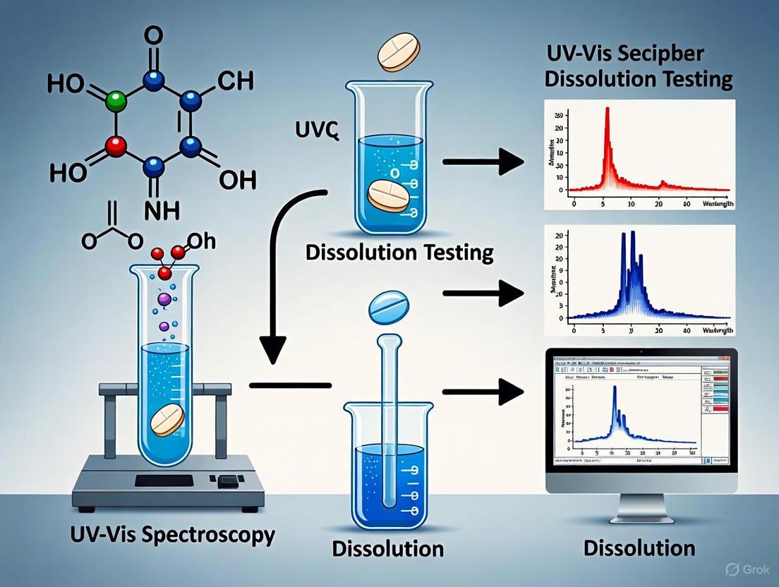
Diagram 1: Drug release quantification workflow.
Materials and Equipment:
- Dissolution apparatus (e.g., USP Type I or II)
- UV-Vis spectrophotometer
- Cuvettes (e.g., quartz with 1 cm path length)
- Volumetric flasks, pipettes
- Membrane filters (e.g., 0.45 μm)
- Dissolution medium (e.g., buffer at pH 1.2, 4.5, or 6.8)
- Standard reference of the API
Procedure:
- Calibration Curve Generation:
- Prepare a stock solution of the API with a known, high concentration.
- Dilute the stock solution serially to create at least five standard solutions covering a concentration range expected during dissolution.
- Measure the absorbance of each standard and the blank (dissolution medium) at the predetermined λ_max.
- Plot absorbance versus concentration and perform linear regression. The R² value should be >0.995.
Dissolution Testing:
- Place the dissolution medium into the apparatus and allow it to equilibrate to 37.0±0.5 °C.
- Introduce the tablet into the vessel and start the agitation (e.g., 50 rpm for paddles).
- Sampling: At predetermined time intervals (e.g., 5, 10, 15, 30, 45, 60 minutes), withdraw a small aliquot (e.g., 2-5 mL) from the vessel.
- Filtration: Immediately pass the sample through a syringe filter to remove any undissolved particles, which can scatter light and cause analytical errors [4].
- Analysis: Transfer the filtered sample to a cuvette and measure its absorbance at λ_max against a blank of fresh dissolution medium.
Data Analysis:
- Use the equation from the calibration curve to calculate the concentration of the API in each sample.
- Calculate the cumulative amount of drug released per volume, and then as a percentage of the tablet's label claim.
- Plot the cumulative drug release (%) versus time to generate the dissolution profile.
Advanced Application: Measuring Diffusion Coefficients
Understanding drug diffusion is critical for predicting in vivo performance. UV-Vis spectroscopy, coupled with the Beer-Lambert Law, can be adapted to measure the diffusion coefficients of small molecules and proteins [3].
Experimental Protocol: Diffusion Cell Method
Protocol Title: UV-Vis Based Measurement of Diffusion Coefficient.
Principle: A custom diffusion cell is created, often by modifying a standard cuvette with a physical barrier or a 3D-printed cover with a slit [3]. The drug diffuses from a high-concentration zone to a low-concentration zone. The changing concentration in the diffusion path is monitored via UV-Vis, and Fick's laws of diffusion are applied to calculate the diffusion coefficient.
Diagram 2: Diffusion coefficient measurement workflow.
Procedure:
- Cell Preparation: A cover with a defined horizontal slit is attached to a cuvette, restricting the light path to a specific height [3].
- Experiment Initiation: The cuvette is filled with a clear dissolution medium or polymer solution. A concentrated drug solution is carefully introduced at the bottom.
- Data Collection: The absorbance at the slit height is measured continuously or at frequent intervals as drug molecules diffuse upwards.
- Calculation: The resulting concentration-time data is fitted to mathematical models derived from Fick's second law of diffusion, using either analytical or numerical approaches, to determine the diffusion coefficient (D) [3]. This method has been shown to produce results with high reproducibility [3].
The Scientist's Toolkit: Essential Reagents and Materials
Table 3: Key Research Reagents and Materials for UV-Vis Based Dissolution Studies
| Item | Function / Purpose | Key Considerations |
|---|---|---|
| API Standard | Serves as the reference material for calibration curve generation. | Must be of high and known purity (e.g., pharmacopeial grade). |
| Dissolution Media Buffers | Mimic physiological pH conditions (e.g., gastric pH 1.2, intestinal pH 6.8). | Buffer concentration and ionic strength can affect diffusivity [3] [9]. |
| Quartz Cuvettes | Hold the sample for absorbance measurement. | Quartz is transparent to UV light; plastic cuvettes are not suitable for UV analysis [2]. |
| Membrane Filters | Remove undissolved particles from withdrawn samples to prevent light scattering [4]. | Pore size (e.g., 0.45 μm) must not adsorb the API. Material compatibility should be verified. |
| Polymer Solutions (e.g., HPMC, PVP) | Used to simulate viscous biological fluids or as formulation components in diffusion studies. | Viscosity can significantly impact diffusion coefficients [3]. |
Critical Considerations and Troubleshooting
While the Beer-Lambert Law is foundational, spectroscopists must be aware of its limitations to avoid analytical inaccuracies. Deviations from linearity can be categorized as follows:
Real Deviations (Fundamental Limitations)
- High Concentration: At high concentrations (>10 mM), electrostatic interactions between solute molecules can alter the molar absorptivity (ε). Additionally, high analyte levels can change the refractive index of the solution, leading to non-linearity [9].
- Optical Effects: The classical derivation of the Beer-Lambert law does not fully account for electromagnetic effects, such as changes in the local field, which can become significant, particularly in condensed phases or at high absorbances [10].
Chemical Deviations
- Equilibria: The analyte may undergo concentration-dependent chemical changes such as association, dissociation, dimerization, or reaction with the solvent, leading to species with different absorption spectra [9]. For example, the absorption spectrum of a molecule like phenol red is highly dependent on the pH of the solvent [9].
- Stray Light: Stray radiation outside the nominal wavelength band reaching the detector can cause deviations, especially at high absorbances where the signal-to-noise ratio is low [9].
- Instrumental Deviations
- Polychromatic Light: The law assumes a monochromatic light source. In practice, spectrophotometers use a band of wavelengths. If the molar absorptivity (ε) changes significantly across this bandwidth, non-linearity will result. This is a primary reason for performing measurements at λ_max, where the absorptivity is relatively flat [9].
- Mismatched Cuvettes: Using sample and reference cells with different path lengths or optical properties will introduce a constant systematic error [9].
Best Practices to Mitigate Deviations
- Ensure absorbance readings for quantification fall within the validated linear range of the instrument, typically below 1.0 [2].
- Always use high-quality, matched quartz cuvettes.
- Confirm the monochromaticity of the light and perform measurements at λ_max.
- Use appropriate blank solutions and ensure the sample is free of undissolved particles or air bubbles.
In the pharmaceutical sciences, dissolution testing stands as a critical analytical procedure for assessing drug release from solid oral dosage forms. Throughout the development of this essential quality control test, a natural bond has been established between dissolution and UV spectroscopy for the quantification of active pharmaceutical ingredients (APIs) [11]. This partnership remains fundamental to modern pharmaceutical analysis due to its practical advantages and analytical robustness.
UV spectroscopy has long been the pharmaceutical chemist's traditional method and first option for analyzing dissolution testing results [12]. The technique's fundamental principle—measuring the absorbance of ultraviolet light by dissolved API molecules at specific wavelengths—provides a direct means of quantifying concentration in dissolution media. This simple yet powerful relationship, governed by the Beer-Lambert law, enables researchers to accurately determine API release profiles under physiologically relevant conditions [13] [11].
This application note explores the technical foundations of this synergistic relationship, presents detailed experimental protocols for various dissolution testing scenarios, and examines emerging technologies that build upon this fundamental analytical bond.
Fundamental Advantages of UV Spectroscopy in Dissolution Testing
Practical and Economic Benefits
The enduring partnership between dissolution testing and UV spectroscopy is underpinned by significant practical and economic advantages that make it particularly suitable for pharmaceutical quality control and research settings.
Table 1: Comparative Analysis of UV Spectroscopy vs. HPLC for Dissolution Testing
| Parameter | UV Spectroscopy | HPLC with UV Detection |
|---|---|---|
| Cost per analysis | Low | High (nicknamed "high priced liquid chromatography") |
| Solvent consumption | Aqueous dissolution media only | Organic solvents for mobile phase + disposal costs |
| Equipment maintenance | Minimal | Columns, pumps, and detectors requiring maintenance |
| Sample preparation | Minimal, often just filtration | Transfer to vials, sometimes dilution |
| Analysis time | Seconds to minutes | Minutes to per sample |
| Method validation | Simpler parameters | Additional system suitability parameters (peak symmetry, column plate counts) |
| Data trending | Immediate | Requires data processing |
The economic argument for UV spectroscopy is compelling. As noted by industry experts, HPLC has earned the nickname "high priced liquid chromatography" in some circles due to costs associated with organic solvents, disposal, equipment acquisition, maintenance, and depreciation [12]. UV spectroscopy eliminates many of these expenses, providing significant cost savings for pharmaceutical manufacturers, particularly for routine quality control testing where large numbers of samples are analyzed daily [12].
The speed of analysis represents another significant advantage. A single absorbance value is used to determine concentration, unlike HPLC which requires separation time for each sample [12]. When coupled with sipper systems, UV spectroscopy allows for rapid analysis of samples immediately following dissolution experiments, increasing laboratory throughput and efficiency [12].
Technical and Workflow Advantages
Beyond economic considerations, UV spectroscopy offers substantial technical benefits that strengthen its position in dissolution testing protocols:
- Reduced Complexity: UV methods eliminate HPLC mobile phase preparation, reduce system suitability requirements, and minimize potential analyst errors associated with multiple transfer steps [12].
- Immediate Data Interpretation: Understanding data for trending or investigating potential sources of laboratory errors can be immediate, allowing issues to be resolved quickly under supervision [12].
- Real-time Monitoring Capability: Fiber-optic UV systems enable continuous in-situ measurement of the dissolution process, generating more frequent data points (up to 1/second) for more accurate real-time dissolution profiles [11].
- Regulatory Acceptance: Well-established UV methods are widely accepted by regulatory agencies with clearly defined validation pathways according to ICH Q2 guidelines [14].
Despite these advantages, situations exist where HPLC offers necessary capabilities beyond UV spectroscopy, particularly when dealing with complex formulations where excipients or degradation products absorb at similar wavelengths as the API, requiring chromatographic separation for accurate quantification [12].
Experimental Protocols
Standard UV Spectroscopy for Dissolution Testing
This protocol outlines the standard procedure for quantifying API release using offline UV spectroscopy analysis of dissolution samples.
Table 2: Research Reagent Solutions for Standard UV Dissolution Testing
| Reagent/Material | Specification | Function in Protocol |
|---|---|---|
| Dissolution Medium | USP-specified buffer (e.g., pH 1.2, 4.5, 6.8) | Simulates gastrointestinal conditions for drug release |
| API Reference Standard | Certified purity (>98%) | Calibration curve generation and method validation |
| Filter Membranes | 0.45 μm porosity, compatible with API | Clarification of withdrawn samples by removing particulate matter |
| UV Cuvettes | Quartz, pathlength 1 cm | Holder for liquid samples during spectrophotometric measurement |
| Degassing System | In-line or vacuum filtration | Removal of dissolved gases from dissolution medium to prevent bubble formation |
Workflow Overview
Step-by-Step Procedure
Dissolution Apparatus Setup
- Fill dissolution vessels with 500-900 mL of appropriately selected and degassed medium per USP requirements
- Equilibrate medium to 37.0°C ± 0.5°C
- Place one dosage unit in each vessel following USP Apparatus 1 (basket) or 2 (paddle) specifications
Sample Collection
- Withdraw appropriate aliquot (typically 5-10 mL) from each vessel at predetermined time points using automated sampler or manual syringe
- Immediately replace with equal volume of fresh medium maintained at 37°C to maintain constant volume
- Filter samples through 0.45 μm membrane filters to remove insoluble particulates
UV Spectrophotometric Analysis
- Measure absorbance of filtered samples at predetermined λmax for API using UV spectrophotometer
- Use appropriate blank (dissolution medium) to zero instrument
- Ensure absorbance values fall within linear range of calibration curve (typically 0.2-1.0 AU)
Data Analysis
- Calculate API concentration using pre-established calibration curve (A = εbc)
- Determine cumulative drug release at each time point, correcting for sample removal
- Plot dissolution profile (percentage released vs. time)
Method Validation Parameters
- Linearity: R² > 0.995 over specified concentration range
- Precision: RSD < 2% for repeatability
- Accuracy: 98-102% recovery of spiked samples
- Specificity: No interference from excipients or degradation products
Fiber-Optic UV Dissolution Testing
Fiber-optic dissolution testing (FODT) represents an advanced approach that enables real-time, in-situ monitoring of the dissolution process without manual sampling [14] [11].
Workflow Overview
Step-by-Step Procedure
System Configuration
- Install fiber-optic probes in each dissolution vessel positioned to monitor representative fluid region
- Connect probes to UV spectrophotometer with photodiode array (PDA) or charge-coupled device (CCD) detector
- Configure software for continuous spectral acquisition (e.g., every 10-30 seconds)
Calibration
- Develop multivariate calibration model using standard solutions covering expected concentration range
- Include potential interferents in model development for complex formulations
- Validate model with independent standard set (accuracy 98-102%)
Dissolution Testing
- Initiate dissolution test following standard USP procedures
- Begin continuous spectral acquisition throughout test duration
- Monitor system performance for consistent light transmission
Data Processing
- Process spectral data using appropriate algorithms to convert absorbance to concentration
- Apply background correction and pathlength normalization as needed
- Generate complete dissolution profile with high temporal resolution
Advantages of FODT
- Eliminates manual sampling and associated errors [14]
- Provides high-density data points for accurate profile generation [11]
- Enables real-time release testing with immediate results [14]
- Redances labor requirements and consumable costs [11]
UV Surface Dissolution Imaging
UV dissolution imaging is an emerging technology that provides visualization of dissolution phenomena at the solid-liquid interface with high spatial and temporal resolution [13].
Step-by-Step Procedure
Sample Preparation
- Compact API powder or formulation into pellet using sample cup
- Apply consistent compression force (e.g., 40 cNm torque) for reproducible surface characteristics
- For formulated products, core sample from tablet using appropriate tooling
Instrument Setup
- Mount sample cup at bottom of quartz flow cell with sample surface facing upward
- Set flow rate of dissolution medium using programmable syringe pump (typically 0.01-0.5 mL/min)
- Select appropriate UV wavelength using band pass filter based on API absorbance characteristics
- Focus UV imaging system on sample surface interface
Image Acquisition
- Initiate flow of dissolution medium across sample surface
- Begin time-resolved image acquisition using CMOS array detector
- Continue acquisition throughout dissolution experiment (typically 30-120 minutes)
Data Analysis
- Analyze sequence of UV images to determine drug concentration gradients near interface
- Calculate flux and intrinsic dissolution rate using appropriate mathematical models
- Correlate dissolution behavior with physical changes observed at surface
Application Notes
- Particularly valuable for studying API behavior including single crystal dissolution and intrinsic dissolution of different crystal forms [11]
- Useful for examining drug-excipient interactions and release mechanisms [13]
- Enables visualization of concentration gradients not apparent in bulk solution measurements [13]
Advanced Applications and Emerging Approaches
UV Spectroscopy in Quality by Design and Real-Time Release
The integration of UV spectroscopy with Quality by Design (QbD) principles and real-time release testing (RTRT) represents the cutting edge of pharmaceutical analysis [15] [14]. Implementation of Analytical Quality by Design (AQbD) approaches for UV-based methods involves establishing an Analytical Target Profile (ATP) that defines method performance requirements [15].
For continuous manufacturing platforms, UV spectroscopy serves as a vital process analytical technology (PAT) tool. The methodology has been successfully applied to monitor API content during hot melt extrusion processes, demonstrating that in-line UV-Vis spectroscopy is a robust and practical PAT tool for monitoring critical quality attributes [15]. These applications highlight the expanding role of UV spectroscopy beyond traditional quality control toward integrated process understanding and control.
Addressing Technical Challenges
Despite its widespread utility, UV spectroscopy faces challenges in complex analytical scenarios:
Multicomponent Formulations For formulations containing multiple APIs with overlapping UV spectra, several approaches can maintain methodology effectiveness:
- Fiber-optic systems with multivariate calibration capable of deconvoluting spectral signals [14]
- Mathematical modeling using partial least squares and peak area models [14]
- Implementation of multi-wavelength monitoring and derivative spectroscopy
Interfering Excipients When excipients interfere with API quantification:
- Employ chromatographic separation (HPLC) when specificity cannot be achieved [12]
- Utilize advanced spectral processing algorithms to account for background interference [14]
- Implement standard addition methods to verify accuracy in complex matrices
Table 3: Troubleshooting Guide for UV Dissolution Methods
| Issue | Potential Causes | Recommended Solutions |
|---|---|---|
| Poor reproducibility between vessels | Inadequate degassing, temperature gradients | Implement strict degassing protocols, verify temperature uniformity |
| Deviation from reference method | Spectral interferences, improper wavelength selection | Verify method specificity, confirm λmax with standard solutions |
| Non-linear calibration | Stray light effects, incorrect dilution scheme | Verify linear range, check instrument performance, prepare fresh standards |
| Fiber-optic signal drift | Probe fouling, source intensity variation | Implement reference channel, clean probes regularly |
The natural bond between dissolution testing and UV spectroscopy remains as relevant today as in the early development of pharmaceutical analysis. The technique's fundamental advantages of cost-effectiveness, speed, simplicity, and reliability ensure its continued prominence in pharmaceutical laboratories worldwide [12]. While HPLC remains necessary for specific applications requiring separation, UV spectroscopy provides an optimal balance of performance and practicality for the majority of dissolution testing scenarios.
Emerging technologies including fiber-optic UV systems, UV dissolution imaging, and advanced spectral processing are strengthening this natural bond by extending applications to more complex formulations and enabling real-time release testing [13] [14] [11]. These advancements, coupled with the established regulatory acceptance and straightforward validation pathways, position UV spectroscopy as the cornerstone technique for dissolution testing now and into the foreseeable future.
As the pharmaceutical industry continues to evolve with increased emphasis on continuous manufacturing and real-time quality assurance, the flexibility and adaptability of UV spectroscopic methods will ensure this natural bond grows even stronger, continuing to serve as the foundation for understanding and controlling drug product performance.
Traditional drug dissolution testing has predominantly relied on methods that measure the active pharmaceutical ingredient (API) in the bulk solution, offering limited insight into the underlying release mechanisms [13]. There is now a significant drive within pharmaceutical research and development towards real-time analysis and continuous monitoring methods that can provide a more profound understanding of drug release phenomena [13]. This shift is crucial for enhancing product quality, optimizing formulations, and accelerating drug development processes.
Advanced techniques such as UV dissolution imaging and UV-Vis spectroscopy with CIELAB color space transformation are emerging as powerful tools that transcend conventional bulk concentration measurements [16] [13]. These methodologies enable researchers to visualize dissolution events at the solid-liquid interface, monitor physical and chemical changes in dosage forms in real-time, and establish correlations between critical quality attributes and process parameters, ultimately providing unprecedented insights into drug release mechanisms.
Advanced UV-Vis Methodologies for Comprehensive Dissolution Analysis
UV Dissolution Imaging
UV dissolution imaging represents a significant advancement in dissolution testing technology, providing both visualization of dissolution phenomena at the solid-liquid interface and quantitative concentration measurements [13]. This technique utilizes light in the wavelength range of 190-800 nm, leveraging the inherent ability of drug substances to absorb light, where the absorption occurs when an electron is promoted to a higher energy state by the energy of an incident photon [13].
The technology has proven particularly valuable for intrinsic dissolution rate (IDR) determinations, form selection, and drug-excipient compatibility studies during early development phases [13]. More recently, with the advent of larger area imaging systems such as the USP type IV-like whole dose cell, UV imaging applications have expanded to include whole dosage forms like tablets and capsules, providing insights into dissolution phenomena not captured by offline measurements [13].
Table 1: Key Applications of UV Dissolution Imaging in Pharmaceutical Development
| Application Area | Specific Uses | Key Benefits |
|---|---|---|
| Form Selection | Comparison of different API solid forms | Enables visualization of dissolution behavior linked to crystal form |
| IDR Determination | Measurement of intrinsic dissolution rates from small quantities of material | Compound-sparing approach; requires as little as 14 μg of material [13] |
| Drug-Excipient Compatibility | Assessment of interactions between API and excipients | Provides real-time visualization of incompatibilities |
| Whole Dose Imaging | Study of tablets and capsules using larger imaging cells | Reveals heterogeneity in dissolution behavior within a dosage form |
| Non-Oral Formulations | Transdermal patches, implants, and other delivery systems | Enables monitoring of release mechanisms for non-oral routes |
CIELAB Color Space Transformation with UV/Vis Spectroscopy
The CIELAB color space, developed by the International Commission on Illumination (CIE), provides an innovative approach for simultaneous monitoring of chemical and physical tablet properties during compression [16]. This method transforms raw UV/Vis spectra (380-780 nm) into a three-dimensional Cartesian coordinate system defined by parameters L, a, and b, where L represents lightness (0-black to 100-white), a* represents the green-red ratio, and b* represents the yellow-blue ratio [16]. These parameters can be further converted to polar coordinates C* (chroma, color saturation) and h° (hue) [16].
The fundamental principle underlying this technique involves the relationship between tablet surface properties and light reflection behavior. On smooth surfaces, specular reflection predominates, where the angle of incidence equals the angle of reflection. In contrast, rough surfaces produce diffuse reflection, scattering radiation in all directions [16]. Additional factors such as volume scattering through fine particles and the cavity effect in surface cavities further influence reflection patterns [16]. These phenomena enable the correlation between color parameters and critical tablet properties such as porosity and tensile strength.
Table 2: CIELAB Color Space Parameters and Their Pharmaceutical Significance
| Parameter | Definition | Pharmaceutical Significance |
|---|---|---|
| L* | Lightness (0 = black, 100 = white) | Related to surface reflectance and overall appearance |
| a* | Green (-) to Red (+) ratio | Color characterization of formulation components |
| b* | Blue (-) to Yellow (+) ratio | Color characterization of formulation components |
| C* | Chroma (color saturation) | Correlates with porosity and tensile strength [16] |
| h° | Hue angle | Overall color characterization |
Experimental Protocols
Protocol: In-line Monitoring of Tablet Porosity and Tensile Strength Using CIELAB Color Space
Objective: To demonstrate the feasibility of UV/Vis diffuse reflectance spectroscopy combined with CIELAB color space transformation for real-time monitoring of tablet porosity and tensile strength during continuous direct compression.
Materials and Equipment:
- Rotary tablet press (e.g., Fette 102i) [16]
- UV/Vis probe with diffuse reflectance capability
- Powder blends with varied particle sizes and deformation properties
- Magnesium stearate as lubricant
- Data acquisition system for continuous monitoring
Methodology:
- Formulation Preparation: Prepare five different formulations varying in particle size and deformation behavior according to Table 3. Use α-lactose monohydrate (Foremost 310 and Tablettose 80) for particle size variations and microcrystalline cellulose (Emcocel 90M) for different deformation characteristics. Include theophylline monohydrate as a model API for absorption studies [16].
Blending Procedure: Blend all formulation components except lubricant for 12 minutes in a 3D shaker mixer at 32 rpm. Add magnesium stearate (0.5 wt%) and blend for an additional 1.5 minutes [16].
Tableting Parameters: Set the rotary tablet press turret speed to 13.9 rpm. Implement the UV/Vis probe at the ejection position of the tablet machine. Process powders at six different main compression forces (3, 6, 9, 12, 15, and 18 kN) to systematically alter physical properties [16].
In-line Measurement: Continuously collect UV/Vis diffuse reflectance spectra during tablet ejection. Transform the raw spectra into CIELAB color space parameters (L, a, b, C) using appropriate software algorithms.
Reference Measurements: Measure tablet porosity using established methods (e.g., terahertz spectroscopy) [16]. Determine tensile strength through diametrical compression testing.
Data Analysis: Establish correlation models between chroma value (C*) and both porosity and tensile strength using linear regression analysis. Validate models with verification runs.
Table 3: Example Formulations for CIELAB Color Space Monitoring [16]
| Formulation Name | API | Major Excipient | Lubricant | Deformation Behavior |
|---|---|---|---|---|
| Lfine | None | Foremost 310 (99.5%) | MgSt (0.5%) | Fragmentation |
| Lcoarse | None | Tablettose 80 (99.5%) | MgSt (0.5%) | Fragmentation |
| LT | Theophylline (10%) | Foremost 310 (89.5%) | MgSt (0.5%) | Plastic deformation |
| M | None | Emcocel 90M (99.5%) | MgSt (0.5%) | Plastic deformation |
| MT | Theophylline (10%) | Emcocel 90M (89.5%) | MgSt (0.5%) | Plastic deformation |
Protocol: Degassing Cyclic Flow UV-Vis Spectroscopy for Bilayer Tablet Dissolution
Objective: To evaluate the dissolution kinetics of bilayer tablets using degassing cyclic flow UV-Vis spectroscopy with chemometrics for simultaneous API quantification.
Materials and Equipment:
- Automatic tablet dissolution tester (e.g., NTR-VS6P) with paddle apparatus [17]
- Degassing tube (Poreflon TB-0201, 1 mm i.d.) [17]
- Peristaltic pump with PharMed tubing (0.5 mm i.d.)
- UV-Vis spectrophotometer with flow cell
- Nicotinamide (NA) and Pyridoxine Hydrochloride (PH) as model APIs
- Carnauba wax as sustained-release matrix
Methodology:
- Tablet Preparation: Prepare bilayer tablets using the dual compression method. For the slow-release layer, compress mixture containing API (e.g., pyridoxine HCl) and carnauba wax at 10 kg/cm². For the fast-diffusion layer, add mixture containing second API (e.g., nicotinamide), microcrystalline cellulose, lactose, and croscarmellose sodium, then compress at 30 kg/cm² [17].
Dissolution Test Setup: Assemble the degassing cyclic flow system as illustrated in Figure 1. Set dissolution parameters to 900 mL water, 37°C, and paddle rotation at 50 rpm. Implement a metal filter at the suction port to prevent clogging [17].
Degassing System: Connect a 5 cm Poreflon degassing tube after the metal filter to prevent air bubble formation in the flow cell, which can interfere with optical path consistency [17].
Spectral Acquisition: Circulate dissolution medium through the flow system at 1.25 mL/min. Acquire UV-Vis spectra in the range of 240-380 nm at 1-minute intervals for 60 minutes [17].
Multivariate Calibration: Develop Partial Least Squares (PLS) regression models using standard solutions of individual APIs. Use baseline optimization to prevent baseline shift of spectra. Validate models using root mean square error (RMSE) calculations [17].
Concentration Prediction: Apply PLS regression models to the collected spectral data to predict individual API concentrations throughout the dissolution process, enabling simultaneous quantification of both APIs despite spectral overlap.
Figure 1: Workflow for real-time monitoring of tablet properties using UV-Vis spectroscopy with CIELAB color space transformation.
The Scientist's Toolkit: Essential Research Reagents and Materials
Table 4: Key Research Reagent Solutions for Advanced UV-Vis Dissolution Studies
| Category | Specific Materials | Function & Application |
|---|---|---|
| Model APIs | Theophylline monohydrate [16], Nicotinamide (NA), Pyridoxine hydrochloride (PH) [17] | Model compounds with known UV absorption characteristics for method development |
| Excipients for Release Modulation | Carnauba wax [17], Microcrystalline cellulose (MCC) [16] [17], Lactose [16] [17], Croscarmellose sodium (CCS) [17] | Control drug release rates; MCC and lactose for fast release, carnauba wax for sustained release |
| Tableting Lubricants | Magnesium stearate (Ligamed MF-2-V) [16] | Prevent adhesion to tooling; critical for continuous manufacturing processes |
| Spectroscopic Accessories | Quartz cuvettes/cells [2], Flow cells with degassing systems [17], UV-Vis probes for in-line implementation [16] | Enable accurate UV measurements; quartz transparent to UV light, degassing prevents bubble interference |
| Chemometric Tools | Partial Least Squares (PLS) regression algorithms [17], CIELAB color space transformation algorithms [16] | Resolve overlapping spectral signals; extract physical property information from spectral data |
Data Analysis and Interpretation
Correlation of CIELAB Parameters with Tablet Properties
Research demonstrates that increasing the main compression force during tableting decreases tablet surface roughness and porosity while increasing tensile strength [16]. These physical changes significantly affect the radiation reflection behavior on the tablet surface, resulting in measurable changes in the chroma value (C) in the CIELAB color space [16]. Linear relationships between C values and both porosity and tensile strength have been observed across multiple formulations, enabling the development of predictive models for real-time quality monitoring [16].
The sensitivity of this technique depends on the formulation characteristics, with different excipients and API combinations exhibiting varying response patterns. For instance, formulations containing theophylline as a model API demonstrated distinct absorption characteristics that could be correlated with physical properties while simultaneously monitoring API content [16].
Chemometric Analysis of Dissolution Data
For bilayer tablet dissolution, PLS regression effectively resolves overlapping UV-Vis spectral peaks of multiple APIs, enabling accurate concentration prediction without traditional chromatographic separation [17]. The degassing flow system proves critical for maintaining measurement accuracy by preventing air bubble accumulation in the flow cell over extended measurement periods (up to 1800 minutes) [17].
The dissolution kinetics obtained through this methodology reveal distinctive release profiles for different layers of bilayer tablets, with the wax matrix layer exhibiting sustained release characteristics compared to the fast-diffusion layer [17]. This approach provides a comprehensive understanding of the dissolution mechanism, including the influence of matrix ingredients on release kinetics.
Figure 2: Schematic representation of the degassing cyclic flow UV-Vis spectroscopy system for dissolution testing.
The integration of advanced UV-Vis methodologies, including UV dissolution imaging and CIELAB color space transformation, represents a paradigm shift in dissolution testing that moves beyond simple bulk concentration measurements. These techniques provide comprehensive insights into drug release mechanisms, enable real-time monitoring of critical quality attributes, and facilitate the development of robust pharmaceutical products with enhanced therapeutic performance.
The protocols and applications detailed in this document demonstrate how these advanced spectroscopic methods can be implemented throughout drug development, from early formulation screening to final product quality control. By adopting these innovative approaches, pharmaceutical scientists can gain deeper understanding of product performance, accelerate development timelines, and ultimately deliver higher quality drug products to patients.
{ article }
Key Parameters: Defining critical measurements including λmax, linearity range, and correlation coefficient
Within the framework of research on UV-Vis spectroscopy for dissolution testing of tablets, the reliability of the analytical data is paramount. The accuracy of in vitro dissolution profiles, which are critical for predicting in vivo performance, hinges on the rigorous validation of the spectroscopic method used. This protocol details the application of UV-Vis spectroscopy for drug release studies, focusing on the definition and determination of three fundamental parameters: the wavelength of maximum absorption (λmax), the linearity range, and the correlation coefficient. These parameters form the cornerstone of a robust analytical method, ensuring that the generated dissolution data is accurate, precise, and fit for purpose in pharmaceutical development and quality control.
Theoretical Background and Key Parameter Definitions
The foundation of a reliable UV-Vis spectroscopic method for dissolution testing rests on a clear understanding of its critical parameters. These parameters are not isolated figures but are interconnected characteristics that collectively define the method's capability to produce accurate and precise concentration data from absorbance measurements.
λmax (Wavelength of Maximum Absorption): This is the specific wavelength at which a drug substance exhibits its highest absorbance. Selecting λmax for analysis is crucial as it provides the greatest sensitivity and minimizes the impact of minor instrumental fluctuations. For instance, in dissolution testing, where drug concentration in the medium increases over time, measuring at λmax ensures the highest signal-to-noise ratio throughout the experiment. As evidenced by studies on terbinafine hydrochloride, its λmax can vary with the solvent, such as 283 nm in water and 223 nm in 0.1 M HCl, underscoring the need for empirical determination in the chosen dissolution medium [18] [19].
Linearity Range: This defines the concentration interval over which a direct proportional relationship exists between the analyte's concentration and the instrument's absorbance response. It is empirically established by preparing and measuring a series of standard solutions across an anticipated concentration range. The range must adequately cover the expected concentrations encountered during the entire dissolution process, from the early time points to the final plateau, typically from 5% to 120% of the expected maximum release [20]. For example, a validated method for terbinafine hydrochloride demonstrated a linear range of 5–30 μg/mL [19], while another study confirmed linearity from 0.2–4.0 μg/mL [18].
Correlation Coefficient (r): The correlation coefficient is a statistical measure that quantifies the strength of the linear relationship between concentration and absorbance. A value close to 1.0 indicates a strong linear relationship. According to ICH guidelines, a correlation coefficient of >0.999 is typically required to demonstrate acceptable linearity for analytical methods [21] [19]. This high value confirms that the calibration curve is reliable for interpolating the concentration of unknown samples from their absorbance.
The following workflow outlines the logical process of method development and validation discussed in this article:
Experimental Protocols
Determination of λmax
Principle: This procedure aims to empirically identify the wavelength at which the drug substance shows maximum absorbance in a specific dissolution medium. This ensures optimal analytical sensitivity.
Materials:
- Drug standard (e.g., Terbinafine hydrochloride)
- Dissolution medium or appropriate solvent (e.g., distilled water, 0.1 M HCl)
- Volumetric flasks (10 mL, 100 mL)
- UV-Vis Spectrophotometer (e.g., Shimadzu 2450) with scanning software
Procedure:
- Standard Stock Solution: Accurately weigh approximately 10 mg of the drug standard. Transfer it to a 100 mL volumetric flask, dissolve, and dilute to volume with the dissolution medium to obtain a stock solution of 100 μg/mL [19].
- Working Solution: Pipette 0.5 mL of the standard stock solution into a 10 mL volumetric flask. Dilute to the mark with the dissolution medium to achieve a concentration of 5 μg/mL [19].
- Spectrum Scanning: Fill a cuvette with the dissolution medium to serve as the blank. Place the working solution in another cuvette. Scan both the blank and the sample solution across the UV range, typically from 200 nm to 400 nm [19].
- Identification of λmax: From the resulting spectrum, identify the wavelength corresponding to the highest peak of absorbance. Record this value as the λmax for all subsequent measurements. An example is shown in the visualization of the analytical workflow.
Establishment of Linearity Range and Correlation Coefficient
Principle: This protocol establishes the concentration range over which the Beer-Lambert law holds and quantifies the linearity of the response. This calibration curve is used to determine unknown sample concentrations.
Materials:
- Standard stock solution (100 μg/mL)
- Series of volumetric flasks (e.g., 10 mL)
- UV-Vis Spectrophotometer
Procedure:
- Preparation of Calibration Standards: Into a series of 10 mL volumetric flasks, pipette varying volumes of the standard stock solution. For example, aliquots of 0.5, 1.0, 1.5, 2.0, 2.5, and 3.0 mL can be used. Dilute each to the mark with the dissolution medium to create a calibration series (e.g., 5, 10, 15, 20, 25, and 30 μg/mL) [19].
- Absorbance Measurement: At the predetermined λmax, measure the absorbance of each standard solution against a blank of the dissolution medium.
- Calibration Curve: Plot the measured absorbance against the corresponding concentration for each standard.
- Linear Regression Analysis: Perform a linear regression analysis on the data. The output will provide the equation of the line (y = mx + c, where y is absorbance, m is the slope, x is concentration, and c is the intercept) and the correlation coefficient (r). The method is considered linear if r > 0.999 [21] [19].
- Range Verification: Confirm that the entire range of concentrations expected in dissolution samples (from 5% to 120% of the label claim) falls within the established linear range [20].
The following diagram illustrates the logical steps involved in the calibration and analysis process:
Data Analysis and Acceptance Criteria
The data collected from the experimental protocols must be evaluated against pre-defined acceptance criteria to ensure the method is suitable for dissolution testing. The following table summarizes key validation parameters and their typical targets based on research data.
Table 1: Summary of Key Analytical Parameters from Literature with Acceptance Criteria
| Drug Substance | λmax (Solvent) | Linearity Range (μg/mL) | Correlation Coefficient (r) | LOD/LOQ (μg/mL) | Application |
|---|---|---|---|---|---|
| Terbinafine HCl | 283 nm (Water) [19] | 5–30 [19] | 0.999 [19] | LOD: 0.42, LOQ: 1.30 [19] | Bulk & Formulation |
| Terbinafine HCl | 222 nm (0.1 M HCl) [18] | 0.2–4.0 [18] | - | - | Bulk & Tablets (SIAM*) |
| Terbinafine HCl | 282 nm (0.1 M Acetic Acid) [18] | 2.0–50 [18] | - | - | Bulk & Tablets (SIAM*) |
| Olmesartan Medoxomil | 248.6 nm (0.1 N NaOH) [22] | 10–30 [22] | 0.9999 [22] | LOD: 0.41, LOQ: 1.25 [22] | Combined Tablet |
| Hydrochlorothiazide | 272.8 nm (0.1 N NaOH) [22] | 10–30 [22] | 0.9991 [22] | LOD: 0.44, LOQ: 1.33 [22] | Combined Tablet |
| *SIAM: Stability-Indicating Analytical Method |
Acceptance Criteria:
- Linearity and Correlation: The correlation coefficient (r) for the calibration curve should be greater than 0.999 [21] [19]. The calibration curve is typically constructed from a minimum of six concentration levels [20].
- Precision: The precision of the method, expressed as the percentage relative standard deviation (%RSD) of replicate measurements, should generally be less than 2% [19].
- Accuracy: Recovery studies, where a known amount of standard is added to a pre-analyzed sample, should yield results in the range of 98–102% [19] [22]. This confirms that the method does not suffer from significant interference from the matrix.
The Scientist's Toolkit: Essential Research Reagents and Materials
The development and application of a UV-Vis method for dissolution testing require specific high-quality materials. The following table lists key reagent solutions and their critical functions in the analytical process.
Table 2: Essential Research Reagent Solutions for UV-Vis Dissolution Analysis
| Reagent/Material | Function in Analysis | Exemplary Specification |
|---|---|---|
| Drug Standard | Serves as the primary reference for preparing calibration standards and determining key parameters like λmax. | High-purity certified reference material (CRM) or pharmacopoeial grade [19]. |
| Dissolution Medium | The liquid environment simulating physiological conditions in which tablet dissolution occurs. Acts as the solvent for standards and samples. | Appropriately buffered solutions (e.g., pH 1.2 HCl, pH 6.8 phosphate) as per pharmacopoeia or biorelevant media [23]. |
| HPLC Grade Solvents | Used for preparing mobile phases (in supportive HPLC methods) or for dissolving drugs insoluble in aqueous media. | Low UV absorbance, high purity to prevent interference [21]. |
| Buffer Salts | Used to prepare the dissolution medium and mobile phases to maintain a constant pH, which is critical for drug stability and method robustness. | Analytical Reagent (AR) grade, e.g., Potassium dihydrogen phosphate, disodium hydrogen phosphate [21] [23]. |
The rigorous definition and determination of λmax, linearity range, and correlation coefficient are non-negotiable prerequisites for employing UV-Vis spectroscopy in dissolution testing. As demonstrated through the experimental protocols and literature data, these parameters are interdependent and form the basis of a validated analytical method. Adherence to strict acceptance criteria—such as a correlation coefficient >0.999, a linear range covering 5-120% of the expected release, and precision with an RSD <2%—ensures that the dissolution profile generated is accurate, reliable, and meaningful. This rigorous approach provides drug development professionals and scientists with the confidence needed to make critical decisions regarding formulation performance and quality, ultimately supporting the development of safe and effective pharmaceutical products.
{ /article }
Modern Methodologies: From Fiber Optics to UV Dissolution Imaging
Within pharmaceutical development, dissolution testing serves as a critical analytical procedure to determine the rate and extent of drug release from solid oral dosage forms, such as tablets. This testing provides a vital link between in-vitro product performance and in-vivo bioavailability [24] [25]. UV-Vis spectroscopy is a cornerstone technique for quantifying dissolved analytes in these tests due to its reliability, ease of use, and high precision [26] [2]. The implementation of this spectroscopy primarily follows two distinct pathways: traditional offline (manual) sampling using cuvettes and online (automated) sampling utilizing flow cells.
This application note details the protocols, equipment, and data handling procedures for both methods, providing a structured framework for their application in dissolution testing for drug development.
The Scientist's Toolkit: Essential Research Reagent Solutions
The following table catalogues the essential materials and reagents required for conducting UV-Vis spectroscopy in the context of dissolution testing.
Table 1: Key Research Reagent Solutions for UV-Vis Dissolution Testing
| Item | Function & Application in Dissolution Testing |
|---|---|
| UV-Vis Spectrophotometer | The core instrument for measuring light absorbance by analytes; used for concentration quantification in dissolution samples [26] [2]. |
| Quartz Cuvettes | Sample holders for offline analysis; quartz is essential for UV light transmission, unlike plastic or glass which absorb UV wavelengths [2]. |
| Flow Cell | An in-line cell, typically with quartz windows, connected to the HPLC column or dissolution vessel outlet; enables real-time, online monitoring of the eluent [26]. |
| Deuterium & Tungsten Lamps | Standard light sources in UV-Vis instruments; a deuterium lamp provides UV light, while a tungsten/halogen lamp covers the visible range [2]. |
| Dissolution Media | Aqueous buffers (e.g., pH 1.2, 4.5, 6.8) or other physiologically relevant fluids that simulate the gastrointestinal environment for the dissolution test [27]. |
| Reference Standards (USP RS) | Certified materials, such as USP Prednisone RS Tablets, used for performance verification (PVT) of the dissolution apparatus and method [24]. |
| Syringe Filters | Used for clarifying manually drawn dissolution samples by removing undissolved particles prior to analysis, preventing interference and instrument damage [24]. |
| Degassed Solvents | Dissolution media from which dissolved gases have been removed (e.g., via vacuum filtration) to prevent bubble formation that can interfere with dissolution or detection [24] [25]. |
Offline (Manual) Sampling with Cuvettes
Principle and Workflow
The offline method involves manually withdrawing aliquots from the dissolution vessel at predetermined time points. These samples are then filtered, often diluted, and transferred to a cuvette for subsequent absorbance measurement in a UV-Vis spectrophotometer [24] [28]. This approach is characterized by its flexibility and the use of standard, widely available laboratory equipment.
The step-by-step workflow for the offline manual sampling method is summarized in the diagram below:
Detailed Experimental Protocol
Materials and Equipment:
- Dissolution apparatus (USP Apparatus 1 or 2) [24]
- Thermostated bath maintaining 37.0 ± 0.5 °C [27]
- UV-Vis spectrophotometer with deuterium and/or tungsten lamps [2]
- Quartz cuvettes (e.g., 1 cm path length) [2]
- Syringe filters (e.g., 0.45 µm pore size, validated for non-adsorption) [24]
- Volumetric flasks and pipettes for dilution
- Dissolution media (e.g., deaerated water or buffer) [24]
Step-by-Step Procedure:
- Apparatus Preparation: Calibrate the dissolution apparatus mechanically and with USP Performance Verification Test (PVT) tablets, such as Prednisone RS, to ensure proper operation [24] [25]. Fill each vessel with the specified volume of dissolution medium, typically 500-1000 mL, and equilibrate to 37.0 ± 0.5 °C [24] [27].
- Test Initiation: Begin the test by placing one dosage unit (e.g., tablet) into each vessel and starting the agitation (e.g., paddle at 50 rpm) simultaneously. Consider this time point as t=0.
- Sample Withdrawal: At predetermined intervals (e.g., 5, 10, 15, 30, 45, 60 minutes), manually withdraw a specified volume (e.g., 10-20 mL) from each vessel. The sampling probe should be positioned at a defined location away from the dissolving tablet to avoid interference [24] [27].
- Sample Filtration: Immediately filter the withdrawn samples using a suitable syringe filter. It is standard practice to discard the first 5 mL of the filtrate to account for adsorption losses on the filter membrane [24].
- Sample Preparation: If necessary, dilute the filtrate with fresh dissolution medium to ensure the absorbance reading falls within the ideal range of the spectrophotometer (typically 0.2-1.0 AU) to maintain linearity according to the Beer-Lambert law [2].
- UV-Vis Analysis: a. Blank Measurement: Use the dissolution medium as the blank reference to zero the instrument [2]. b. Sample Measurement: Transfer the prepared sample to a clean quartz cuvette and measure its absorbance at the validated wavelength (e.g., 242 nm for prednisone) [24] [26].
- Data Recording: Record the absorbance value for each sample at each time point.
Data Processing and Analysis
- Concentration Calculation: Convert absorbance values to concentration using a pre-established calibration curve or the analyte's known molar absorptivity (ε) based on the Beer-Lambert law (A = ε * b * c) [2].
- Cumulative Release: Calculate the cumulative percentage of drug dissolved at each time point, accounting for volume replacements and dilutions [29].
- Profile Generation: Plot the mean percentage dissolved versus time to generate the dissolution profile for the batch. Include error bars (e.g., ±SD) from multiple vessel measurements (n=6-12) to indicate variability [24] [27].
Online (Automated) Sampling with Flow Cells
Principle and Workflow
Online methods employ flow-through cells integrated directly into the fluidic path after the dissolution vessel or HPLC column. This setup allows for real-time, in-situ monitoring of the drug concentration without the need for manual sample handling [25] [26]. This approach is highly advantageous for extended-release formulations and supports Process Analytical Technology (PAT) initiatives for real-time release testing (RTRT) [16] [25].
The following diagram illustrates the logical flow and components of an online system with a flow cell:
Detailed Experimental Protocol
Materials and Equipment:
- Dissolution apparatus with integrated fluidics
- UV-Vis spectrophotometer equipped with a flow cell (e.g., Diode Array Detector - DAD) [26]
- Peristaltic pump or automated sampling system
- In-line filters
- Tubing (chemically inert, e.g., PTFE)
Step-by-Step Procedure:
- System Setup and Prime: Connect the flow cell to the fluidic path. Prime the entire system with the dissolution medium to remove air bubbles, which can cause significant signal noise and erroneous absorbance readings [25] [2].
- Baseline Establishment: With the dissolution medium circulating through the flow cell, establish a stable baseline on the UV-Vis detector. This baseline signal will serve as the reference (I₀) for all subsequent measurements [2].
- Test Initiation: Begin the dissolution test as described in the offline protocol (Step 3.2, point 2).
- Continuous Monitoring: Initiate continuous pumping of the medium from the dissolution vessel through the in-line filter and into the flow cell. The detector records the absorbance at set intervals (e.g., every few seconds), building a real-time profile of the drug concentration in the vessel [25].
- System Suitability: Prior to critical tests, validate the online system's performance by circulating a standard solution of known concentration and verifying that the measured absorbance aligns with the expected value.
Data Processing and Analysis
- Real-Time Data Stream: The data system directly collects a continuous stream of absorbance data.
- Conversion to Profile: Software automatically converts the absorbance values to concentration and percentage dissolved, using pre-defined parameters, and generates the dissolution profile in real-time [16]. This facilitates immediate data interpretation and decision-making.
Comparative Analysis: Offline vs. Online Methods
Table 2: Quantitative and Qualitative Comparison of Offline and Online Sampling Methods
| Parameter | Offline (Cuvette) Sampling | Online (Flow Cell) Sampling |
|---|---|---|
| Automation Level | Manual or semi-automated [24] | Fully automated [25] |
| Sampling Frequency | Discrete time points [27] | Continuous, real-time [25] |
| Typical Flow Cell Volume | N/A (Cuvette-based) | 8–18 µL (HPLC), 0.5–1 µL (UHPLC) [26] |
| Risk of Sample Alteration | Higher (filtration, dilution, handling) [24] | Lower (closed system, minimal handling) |
| Suitability for Extended Release | Possible, but labor-intensive for long durations | Ideal for prolonged tests (e.g., 24 hours) [25] |
| PAT / RTRT Suitability | Low | High, enables real-time release testing [16] [25] |
| Key Advantage | Flexibility, uses standard equipment [28] | Real-time data, minimal manual intervention [25] |
| Primary Limitation | Labor-intensive; potential for high variability [24] | Higher initial setup cost and complexity [25] |
Both traditional offline sampling with cuvettes and modern online sampling with flow cells are indispensable methods within the pharmaceutical laboratory. The choice between them depends on the specific application requirements, such as the need for high-throughput quality control, real-time process monitoring, or testing of complex modified-release formulations. Offline methods offer a robust, accessible, and flexible approach, while online flow cell techniques provide the automation, speed, and continuous data acquisition essential for advanced PAT and RTRT strategies. A thorough understanding of both protocols ensures the selection of the most appropriate and informative methodology for dissolution testing in drug development.
Within pharmaceutical development, the dissolution test is a cornerstone for assessing the performance of solid oral dosage forms. Traditional methods, which rely on manual sampling and offline analysis, are labor-intensive and provide only limited data points. This application note details the implementation of real-time dissolution profiling using in-situ fiber-optic UV-Vis spectroscopy, a methodology that aligns with the principles of Process Analytical Technology (PAT) [30] [11]. By enabling continuous, in-situ measurement, this technique provides a rich, detailed dataset that is invaluable for formulation development, troubleshooting, and quality control, ultimately supporting a more efficient and science-based drug development process [31] [12].
Theoretical Background and Principles
Fiber-optic dissolution testing is grounded in the Beer-Lambert Law, which states that the absorbance of light by a solution is directly proportional to the concentration of the absorbing species and the pathlength of the light through the solution [31]. A typical system consists of a UV-Vis light source, a spectrometer, and fiber-optic cables connected to probes immersed directly in the dissolution vessels.
The key innovation is the probe design, which allows for the transmission of light to and from the vessel without the need for fluid removal. Different probe geometries (e.g., with overlapping or non-overlapping illumination and collection areas) can be optimized to be sensitive to specific measurement depths or to minimize hydrodynamic interference [32]. The signal captured by the probe is transmitted back to the spectrometer, where the resulting spectra are processed to quantify the concentration of the dissolved Active Pharmaceutical Ingredient (API) in real-time [33].
Key Advantages Over Traditional Methods
The adoption of fiber-optic probes for dissolution testing offers several distinct advantages that enhance both operational efficiency and data quality.
Table 1: Comparison of Dissolution Testing Methods
| Feature | Traditional Manual Sampling & HPLC | In-Situ Fiber-Optic UV |
|---|---|---|
| Data Density | Limited data points (e.g., 5-7 time points) | High-density, continuous data (points as frequent as every 5 seconds) [33] |
| Analysis Speed | Slow; includes sampling, filtration, and often lengthy HPLC run times | Real-time; immediate data and trending [12] |
| Labor & Cost | High labor; cost of solvents, HPLC vials, and disposal [12] | Reduced labor; eliminates consumables like filters, tubing, and syringes [33] |
| Process Understanding | Provides a basic release profile | Enables observation of complex release dynamics as they occur [11] [33] |
| Automation Potential | Complex, often requiring automated sampling systems | Truly automated from start of test to final report [33] |
Furthermore, with the application of multicomponent analysis (MCA) algorithms, fiber-optic UV systems can simultaneously quantify two APIs in a combination product or account for spectral interference from excipients, coatings, or capsules without the need for chromatographic separation [33].
Experimental Protocols
Protocol 1: Establishing a Real-Time Dissolution Profile for an Immediate-Release Tablet
This protocol describes the steps to monitor the dissolution of a single-API immediate-release tablet using a fiber-optic dissolution system.
Research Reagent Solutions & Essential Materials
Table 2: Essential Materials for Fiber-Optic Dissolution Testing
| Item | Function | Example/Note |
|---|---|---|
| Fiber-Optic Dissolution System | Performs in-situ UV measurement. | E.g., Opt-Diss 410 or equivalent [33]. |
| Dissolution Apparatus | Provides controlled test environment. | USP Apparatus 1 (baskets) or 2 (paddles). |
| Dissolution Medium | Simulates the gastrointestinal environment. | e.g., 0.1N HCl or pH-buffered solutions, degassed [34]. |
| Fiber-Optic Probe | Transmits and collects light in the vessel. | ARCH probe or adjustable pathlength dip probe (e.g., 2-20 mm) [33]. |
| API Reference Standard | For system calibration and validation. | High-purity material for preparing standard solutions. |
Procedure:
- Instrument Setup: Power on the dissolution bath and allow it to reach the specified temperature (typically 37°C ± 0.5°C). Ensure the fiber-optic probes are clean and securely connected to the spectrometer.
- Pathlength Selection: Select an appropriate optical pathlength for the probe based on the expected API concentration and its absorptivity to ensure absorbance values remain within the instrument's linear range (e.g., 0.2-1.0 AU) [33].
- System Calibration:
- Prepare a series of standard solutions of the API in the dissolution medium across a range of known concentrations.
- Immerse the probe in each standard and collect the UV spectrum.
- Using the instrument's software, build a univariate calibration model (absorbance at λmax vs. concentration) or a multivariate model using full-spectrum data.
- Baseline Measurement: Fill the dissolution vessel with the specified volume of dissolution medium. With the paddles rotating at the specified speed (e.g., 50 rpm), immerse the probe and collect a baseline spectrum.
- Initiate Test: Introduce one tablet into each vessel and start the data acquisition software simultaneously.
- Data Acquisition: The system will automatically collect spectra at pre-defined intervals (e.g., every 5-10 seconds initially) [33]. The software will convert the spectral data into concentration values in real-time using the established calibration model.
- Profile Generation: The software plots the cumulative percentage of drug released versus time, generating a continuous dissolution profile.
Protocol 2: Multicomponent Analysis for a Fixed-Dose Combination Product
This protocol extends the capability to products containing two APIs with overlapping UV spectra.
Procedure:
- Follow Steps 1-2 from Protocol 1.
- Multicomponent Calibration:
- Prepare a calibration set of standard solutions that contains varying concentrations of both API A and API B, designed to span the expected concentration ranges.
- Collect full UV spectra for all standard mixtures.
- Use the instrument's software to build a multivariate calibration model (e.g., Partial Least Squares, or PLS) that correlates the spectral features with the known concentrations of both APIs [35] [33].
- Validation: Validate the model using an independent set of standard solutions not used in the calibration.
- Dissolution Test: Perform the dissolution test as described in Steps 4-6 of Protocol 1.
- Concentration Deconvolution: The software will apply the multicomponent model to each collected spectrum, simultaneously calculating the concentrations of both API A and API B, and generating two individual dissolution profiles from a single test [33].
Data Analysis and Chemometrics
The large volume of spectral data generated requires robust chemometric tools for interpretation.
- Univariate Analysis: For single-component analysis, the absorbance at the wavelength of maximum absorption (λmax) is plotted against time. This data can be directly converted to a dissolution profile using the Beer-Lambert law [34].
- Multivariate Analysis: For complex systems, techniques such as Principal Component Analysis (PCA) and Partial Least Squares (PLS) regression are employed. These methods use the entire spectral region to build models that can predict API concentration even in the presence of interfering species or for multi-API products [31] [35].
- Self-Modeling Curve Resolution (SMCR): In some cases, advanced algorithms like SMCR can resolve the concentration profiles of reacting components without the need for pre-defined standards, which is particularly useful for monitoring chemical reactions or complex release mechanisms [31].
Table 3: Quantitative Data from a Representative Study (Drotaverine Extended-Release Tablets)
| Formulation Variable | Level 1 | Level 2 | Level 3 | Key Finding from Dissolution Prediction |
|---|---|---|---|---|
| DR Content (w/w %) | 6% | 8% | 10% | Prediction models using NIR/Raman spectra and compression force accurately predicted dissolution profiles (f2 > 50) [35]. |
| HPMC Content (w/w %) | 10% | 20% | 30% | HPMC content was a critical factor controlling release rate, successfully captured by the model [35]. |
| Compression Force (MPa) | 63.8 | 95.7 | 127.6 | Higher compression force slightly slowed drug release, and the model accounted for this effect [35]. |
Application in Pharmaceutical Development
The rich, real-time data provided by fiber-optic dissolution is instrumental in several key areas of drug development:
- Formulation Screening and Optimization: The ability to capture detailed release dynamics, especially at early time points, allows formulators to quickly discriminate between different prototype formulations [11]. For instance, the technology has been used to screen co-processed API formulations to identify carriers that provide the desired drug release profile [11].
- Troubleshooting and Root Cause Analysis: Continuous profiles can reveal subtle anomalies in drug release that might be missed by traditional sampling. This is critical for investigating batch-to-batch variability or issues observed in stability studies, such as identifying the cross-linking effect on the dissolution of gelatin capsules [11].
- Support for Real-Time Release Testing (RTRT): As a robust PAT tool, fiber-optic dissolution can form the basis of an RTRT strategy, where the dissolution profile is predicted based on in-process data, eliminating the need for end-product testing and reducing batch release times [30] [35].
Fiber-optic UV probes represent a significant advancement in dissolution testing methodology. By enabling continuous, in-situ monitoring, they provide a comprehensive and accurate view of the drug release process, far surpassing the detail offered by traditional methods. The integration of this technology with advanced chemometric analysis empowers researchers and scientists to develop better formulations more efficiently, resolve complex manufacturing issues, and move toward modern, risk-based quality control paradigms like RTRT. Adopting this technology is a decisive step toward deepening the understanding of drug product performance throughout the development lifecycle.
UV Surface Dissolution Imaging (SDI) represents a technological breakthrough in dissolution testing, enabling researchers to directly observe the solid-liquid interface in real-time as a drug substance dissolves [36]. This advanced analytical technique provides a two-dimensional movie of UV absorbance, offering a detailed view of dissolution processes that occur microns from the drug surface [37]. Unlike traditional dissolution methods that only measure bulk concentration, UV SDI captures spatially resolved concentration data, allowing for visualization of the concentration gradient that forms near the surface of a dissolving substance—a central element in dissolution theory that has been difficult to verify experimentally until now [37].
The technology is particularly valuable in pharmaceutical development because most drug substances contain UV chromophores, making UV absorbance a sensitive and robust measurement approach [37]. By combining an imaging detector with specialized flow cells and analysis software, UV SDI provides unique insights into the kinetics and mechanisms of drug release, helping to shift the dissolution paradigm from a data-driven approach toward a knowledge-driven perspective [37]. This mechanistic performance knowledge contributes to a deeper understanding of critical product quality attributes and process parameters, aligning perfectly with Quality by Design (QbD) initiatives in pharmaceutical development [37].
Core Components of UV SDI Systems
The UV SDI system comprises several integrated components designed to provide controlled hydrodynamic conditions and high-resolution imaging:
- Sample Flow Cell: A specially designed cell that provides laminar flow across the surface of compacted drug material. The quartz flow cell is pressed against the imager face, providing a complete side view of the powder surface including areas upstream and downstream [37].
- UV Light Source and Detection: A broad-spectrum pulsed xenon lamp provides flashes of light that are synchronized with a complementary metal oxide semiconductor (CMOS) image sensor (7 mm × 9 mm made up of 1.3 million 7 × 7 μm pixels) for recording light transmission through the flow cell [37].
- Fluid Delivery System: An accurate, stable syringe pump typically using a 20-mL syringe enables controlled volumetric flow across the sample. Multiple flow rate steps can be programmed and synchronized with UV image acquisition [37].
- Data Analysis Software: Proprietary software tools allow extraction and analysis of dissolution data from the captured image sequences, including calculation of intrinsic dissolution rates and visualization of concentration gradients [37].
Fundamental Operating Principles
UV SDI operates on the principle that most pharmaceutical substances absorb UV light, and this absorbance follows the Beer-Lambert law, which relates absorption to concentration [37]. The system converts intensity measurements at each pixel into absolute absorbance values by first subtracting dark values and then applying the standard logarithmic equation comparing initial transmission (I0) and sample transmission (I) [37]. The resulting absorbance values for each pixel in the selected viewing area create a 2-D image, and sequences of these images form a movie that visually represents the dissolution process [37].
The flow cell creates laminar parabolic flow parallel to the image sensor, with flow passing across the drug compact with a surface velocity near zero [37]. This creates steady-state conditions that enable reliable imaging at each moment of flow, with the parabolic flow profile accounting for faster flow at the center of the flow stream compared to the surface wall [37]. The viewing area and binning level can be selected by the operator, with imaging rates typically around 2 Hz for dissolution experiments [37].
Figure 1: UV SDI Technology Workflow - This diagram illustrates the core process of UV Surface Dissolution Imaging, from illumination to data analysis.
Key Research Applications
Intrinsic Dissolution Rate (IDR) Determination
UV SDI provides a compound-sparing approach for determining Intrinsic Dissolution Rates, requiring only 2mg of sample and approximately 20mL of dissolution medium for a typical 30-minute experiment [38]. The system calculates standard IDR values (mass/time/area) from volumetric flow rate and absorbance intensities in specific measurement zones [37]. After entering parameters for molecular weight and extinction coefficient, mass is calculated by applying Beer's law to obtain mass per volume. The known volumetric flow rate is multiplied by the concentration to yield mass/min, which is then divided by the known sample surface area to give mass/min/area (mg/min/cm²) [37]. The laminar flow regime in the apparatus necessitates correction for the parabolic flow profile, where each row of pixels in the measurement zone is adjusted for transit rate based on the known volumetric flow rate [37].
Formulation Selection and Characterization
UV SDI has proven particularly valuable for characterizing the dissolution behavior of different solid forms, including crystalline and amorphous materials. The technology enables visual representation and quantitative assessment of dissolution properties under physiologically relevant conditions, making it ideal for form selection studies [39]. For poorly soluble compounds, UV SDI can capture supersaturation and precipitation events that are critical for predicting in vivo performance [39]. The ability to observe solution-mediated transformation of amorphous to crystalline state when solids are exposed to solvent provides crucial information for stabilizing amorphous formulations [39].
Drug-Excipient Compatibility Studies
During early formulation development, UV SDI helps identify interactions between active pharmaceutical ingredients and excipients. The technology can visualize how excipients affect dissolution behavior, including phenomena such as gelling layer formation and matrix effects that influence drug release [39]. For example, studies with Sporanox pellets containing itraconazole demonstrated how polyethylene glycol (PEG) gelling layers and hydroxypropyl methylcellulose (HPMC) matrices affect dissolution patterns [39].
Whole Dosage Form Imaging
With the introduction of USP type IV-like whole dose cells in dissolution imaging, UV SDI can now be applied to study tablets and capsules [13]. This advancement enables drug release studies from complete dosage forms, bridging preformulation and compatibility studies with dosage form evaluation [13]. The visualization of whole tablet dissolution provides insights into disintegration behavior and release mechanisms that are not apparent from traditional dissolution testing.
Table 1: Summary of Key UV SDI Applications in Pharmaceutical Development
| Application Area | Key Information Obtained | Typical Experiment Duration | Sample Requirement |
|---|---|---|---|
| Intrinsic Dissolution Rate (IDR) Determination | IDR values, concentration gradients, flow rate effects | 20-30 minutes | 2-4 mg [38] |
| Form Selection | Dissolution mechanisms of different solid forms, precipitation tendencies | 30 minutes | 2-4 mg [39] |
| Drug-Excipient Compatibility | Excipient effects on dissolution, gel layer formation, matrix performance | 30-60 minutes | 2-4 mg of formulation [39] |
| Whole Dosage Form Imaging | Tablet disintegration, drug release mechanisms from complete dosage forms | Varies by formulation | Whole tablet/capsule [13] |
Experimental Protocols
Protocol 1: Determination of Intrinsic Dissolution Rate
Objective: To determine the intrinsic dissolution rate of a pure drug substance under controlled hydrodynamic conditions.
Materials and Equipment:
- UV SDI system (e.g., ActiPix SDI 300 or Sirius SDI)
- Pure drug substance (2-4 mg)
- Appropriate dissolution medium (20 mL)
- Miniature press and torque screwdriver for compact preparation
- Stainless steel sample tubes (2.0 mm i.d.)
Procedure:
Sample Preparation:
- Place the drug substance (2-4 mg) in a stainless steel sample tube.
- Compact the powder using a miniature press and torque screwdriver. Typical torque settings range from 20-80 cNm, depending on the material properties [37].
- Ensure a uniform, flat surface on the compact.
System Setup:
- Place the compact in the flow cell assembly, positioning it exactly under the fiber optic in the center of the quartz tube.
- Select appropriate UV filter based on the drug's absorbance characteristics (e.g., 254 nm for atenolol, 280 nm for furosemide) [37].
- Set imaging parameters: typical imaging rates of 2 Hz with binning level selected to balance spatial resolution and sensitivity [37].
Background Measurement:
- Fill the flow cell with dissolution medium.
- Collect dark values over a 10-second period to account for electronic noise.
- Collect background intensities from the buffer contained within the flow cell over a subsequent 10-second period [37].
Dissolution Experiment:
- Initiate flow of dissolution medium using the syringe pump. Typical flow rates range from 0.6-2.0 mL/min, depending on the drug solubility [37].
- Begin image acquisition synchronized with flow initiation.
- Continue the experiment for sufficient time to establish steady-state dissolution (typically 20-30 minutes).
Data Analysis:
- Convert intensity values to absorbance using the Beer-Lambert law.
- Extract concentration profiles from selected measurement zones.
- Calculate intrinsic dissolution rate using the formula: IDR = (C × Q) / A, where C is concentration (determined from absorbance), Q is volumetric flow rate, and A is surface area of the compact [37].
- Apply parabolic flow correction to account for laminar flow conditions [37].
Protocol 2: Biorelevant Dissolution with Media Transition
Objective: To investigate dissolution behavior under conditions simulating the gastrointestinal transition from gastric to intestinal environment.
Materials and Equipment:
- UV SDI system with media switching capability
- Drug substance or formulation (4 mg)
- Simulated gastric fluid (SGF) or fasted state simulated gastric fluid (FaSSGF)
- Simulated intestinal fluid (SIF) or fasted state simulated intestinal fluid (FaSSIF-V1)
Procedure:
Sample Preparation:
- Prepare compacts as described in Protocol 1, using 4 mg of drug substance or formulation [39].
Initial Gastric Phase:
- Begin dissolution with gastric medium (SGF or FaSSGF) at an appropriate flow rate.
- Monitor dissolution for 10-15 minutes to establish baseline behavior in gastric conditions.
Media Transition:
- Switch to intestinal medium (SIF or FaSSIF-V1) while maintaining flow.
- Observe any changes in dissolution behavior, including potential precipitation events.
- Continue monitoring for 15-30 minutes to capture complete transition effects.
Flow Rate Variations:
- Implement step changes in flow rate to simulate different hydrodynamic conditions in the GI tract.
- Typical flow rates range from static (0 mL/min) to 4 mL/min [39].
Data Analysis:
- Compare dissolution behavior in different media.
- Identify precipitation events by visualizing the formation and dissipation of high-concentration zones.
- Calculate dissolution rates in each media condition.
Table 2: Typical Experimental Conditions for UV SDI Studies of Model Compounds
| Parameter | Atenolol (Highly Soluble Base) | Furosemide (Poorly Soluble Acid) | Cefuroxime Axetil (Poorly Soluble) | Itraconazole (Poorly Soluble) |
|---|---|---|---|---|
| Medium pH | pH 4.5 phosphate buffer | pH 2.0 phosphate buffer | Sequential: FaSSGF → FaSSIF-V1 | Sequential: FaSSGF → FaSSIF-V1 |
| Flow Rate | 0.6 mL/min | 2.0 mL/min | Multiple steps including static | Multiple steps including static |
| Wavelength | 254 nm | 280 nm | Compound-specific | Compound-specific |
| Torque for Compaction | 20 cNm | 80 cNm | Not specified | Not specified |
| Key Observations | Large plume of concentrated solution | Limited concentration zone near surface | Swelling in SGF/FaSSGF, convective flow in FaSSIF-V1 | Upward diffusion in biorelevant media |
Representative Research Findings
Case Study 1: Dissolution of Highly Soluble vs. Poorly Soluble Drugs
UV SDI effectively differentiates dissolution behaviors between highly soluble and poorly soluble compounds. In studies with atenolol (highly soluble base) and furosemide (poorly soluble acid), marked differences in dissolution patterns were observed [37]. For atenolol, a large plume of concentrated solution was visible, transported away by the flowing buffer, with a pale blue area representing dilute solution diffusing into the bulk buffer [37]. In contrast, furosemide showed a region of high concentration limited to the area very close to the sample surface and immediately downstream of the sample cup, reflecting its much lower solubility [37].
Analysis of the solution absorbance profile perpendicular to the flow direction for furosemide demonstrated that absorbance (hence concentration) decreases rapidly when moving into the bulk solution, in accordance with convective-diffusion theory [37]. As flow rate decreased, the impact of diffusion became more significant, allowing furosemide to spread further into the bulk solution [37].
Case Study 2: Amorphous Formulation Analysis
Studies with amorphous cefuroxime axetil and itraconazole formulations demonstrated the value of UV SDI in characterizing complex dissolution behavior. For cefuroxime axetil in simulated gastric fluid (SGF) and fasted state simulated gastric fluid (FaSSGF), the dissolution mechanism was predominantly swelling, contrasted with convective flow observed in fasted state simulated intestinal fluid (FaSSIF-V1) [39]. This difference was attributed to the effect of mixed micelles in the biorelevant media.
For itraconazole compacts in biorelevant media, clear upward diffusion of the dissolved drug into the bulk buffer solution was observed [39]. When studying the commercial formulation Sporanox, dissolution was affected by the polyethylene glycol (PEG) gelling layer and hydroxypropyl methylcellulose (HPMC) matrix, revealing a steady diffusional dissolution pattern [39]. These observations provide crucial insights into the performance of amorphous formulations that cannot be obtained through traditional dissolution testing.
Figure 2: UV SDI Experimental Protocol - This workflow outlines the key steps in conducting UV Surface Dissolution Imaging experiments, from sample preparation to data analysis.
The Scientist's Toolkit: Essential Research Reagents and Materials
Table 3: Essential Research Reagents and Materials for UV SDI Experiments
| Item | Function/Purpose | Examples/Specifications |
|---|---|---|
| UV SDI Instrument | Core imaging system for dissolution visualization | ActiPix SDI 300, Sirius SDI [37] [38] |
| Sample Compaction Equipment | Preparation of consistent drug compacts | Miniature press, torque screwdriver (20-80 cNm), stainless steel sample tubes (2.0 mm i.d.) [37] |
| Biorelevant Dissolution Media | Simulate gastrointestinal conditions for physiologically relevant data | Simulated Gastric Fluid (SGF), Fasted State Simulated Gastric Fluid (FaSSGF), Simulated Intestinal Fluid (SIF), Fasted State Simulated Intestinal Fluid (FaSSIF-V1) [39] |
| Buffer Components | Create controlled pH environments for dissolution testing | Phosphate buffers, pH-specific media components [37] |
| UV-Absorbing Drug Standards | System calibration and method validation | Atenolol, furosemide, cefuroxime axetil, itraconazole [37] [39] |
| Syringe Pump and Fluidics | Controlled flow delivery for consistent hydrodynamic conditions | 20-mL syringe, programmable flow rates (0-4 mL/min) [37] |
| Data Analysis Software | Processing and interpretation of imaging data | Proprietary software with concentration calculation, IDR determination, and visualization tools [37] |
Advantages and Methodological Considerations
Key Advantages of UV SDI
UV Surface Dissolution Imaging offers several significant advantages over traditional dissolution methods:
- Visualization Capability: Provides direct observation of dissolution phenomena at the solid-liquid interface, revealing processes that are not detectable with traditional methods [37] [38].
- Compound Sparing: Requires only 2mg of sample, making it ideal for early development when API is limited [38] [36].
- Rapid Analysis: Enables IDR determination in 20-30 minutes compared to 24-hour equilibrium IDR using traditional dissolution systems [39].
- Biorelevant Conditions: Facilitates testing under physiologically relevant conditions with easy media transitions and flow rate changes [39].
- Mechanistic Insights: Reveals dissolution mechanisms, including swelling, convection, diffusion, and precipitation events [39].
Methodological Considerations and Limitations
While powerful, UV SDI has certain limitations that researchers should consider:
- UV Chromophore Requirement: The drug substance must contain a UV chromophore for detection [37].
- Throughput Considerations: May have lower throughput compared to some small-scale dissolution methods that run multiple samples in parallel [13].
- Hydrodynamic Modeling: Quantification relies on the suitability of the hydrodynamic model of the prevailing flow conditions and image analysis [13].
- Variability Potential: May be associated with higher variability in IDR values compared to some traditional methods due to reliance on image analysis and flow modeling [13].
UV Surface Dissolution Imaging represents a significant advancement in dissolution testing technology, providing unprecedented visualization of the dissolution process at the solid-liquid interface. By enabling real-time observation of concentration gradients and dissolution phenomena, SDI moves beyond traditional concentration measurements to offer mechanistic insights into drug release behavior. The technology's minimal sample requirements, rapid analysis times, and ability to simulate physiologically relevant conditions make it particularly valuable for early formulation development, form selection, and biopharmaceutical assessment.
As pharmaceutical development continues to embrace Quality by Design principles and seeks more predictive in vitro tools, UV SDI offers a powerful approach to bridge the gap between traditional dissolution testing and in vivo performance. The continuous evolution of UV SDI applications, including whole dosage form imaging and non-oral formulation assessment, promises to expand its utility across the pharmaceutical development continuum.
In the pharmaceutical development of solid oral dosage forms, dissolution testing serves as a critical analytical tool for assessing drug release behavior, guiding formulation design, and ensuring product quality and performance. UV-Vis spectroscopy has long been an indispensable technique for dissolution analysis due to its cost-effectiveness, speed, and simplicity [11] [12]. Recent technological advancements, particularly the development of UV dissolution imaging, have transformed this methodology from a simple bulk concentration measurement into a powerful tool for visualizing and quantifying API release phenomena with high spatial and temporal resolution [11] [13]. This application note details specific case studies and protocols demonstrating the value of UV-Vis spectroscopy and imaging in formulation development, with emphasis on co-processed API screening and investigation of extended-release mechanisms, providing researchers with practical frameworks for implementation.
Theoretical Background and Technological Advantages
Principles of UV-Vis Spectroscopy and Imaging in Dissolution
UV-Vis spectrophotometry for dissolution testing operates on the fundamental principle that drug substances absorb light in the ultraviolet and visible regions (190-800 nm) [13]. When an electron is promoted to a higher energy state by an incident photon, the resulting absorption can be quantified and correlated to API concentration through the Beer-Lambert Law, enabling straightforward quantification of drug release [11] [13]. This relationship provides a direct means to measure the concentration of API dissolved in the medium over time, generating a dissolution profile.
UV surface dissolution imaging (SDI), a more recent innovation, extends this capability by combining UV spectroscopy with spatial resolution. In a typical SDI system, a sample is compacted into a pellet or a solid sample is cored and placed in a sample cup at the bottom of a quartz flow cell [11] [13]. Dissolution medium flows through the cell under controlled conditions, while a selected wavelength of UV light illuminates the interface between the sample and dissolution medium. A CMOS array detector captures images of the drug concentration gradient at or near this interface, enabling visualization and quantification of the dissolution process in real-time [11].
Comparative Advantages of UV-Based Techniques
UV-based dissolution methods offer distinct advantages for formulation scientists. Traditional UV spectroscopy provides a cost-effective and efficient alternative to HPLC, eliminating needs for organic solvents, reducing equipment costs, and simplifying validation procedures [12]. The technique's speed enables immediate data trending and rapid decision-making during formulation development.
UV dissolution imaging adds significant value through its ability to visualize dissolution phenomena at the solid-liquid interface, providing insights into release mechanisms not captured by traditional bulk concentration measurements [11] [13]. This technique enables high-temporal-resolution data collection (up to 1 measurement per second) compared to limited data points from discrete sampling [11]. Additionally, UV imaging requires only small sample quantities, a particular advantage when working with potent compounds or during early development stages when API availability is limited [11] [13].
Figure 1: Decision workflow for implementing UV-based techniques in pharmaceutical formulation development, highlighting application areas for traditional UV spectroscopy and advanced UV dissolution imaging.
Application Case Study: Co-Processed API Screening
Background and Rationale
The development of formulations for potent BCS Class II drugs presents multiple challenges, including poor processability, pH-dependent solubility, and high toxicity [11]. Co-processing of API with functional excipients has emerged as a valuable strategy to address these issues, particularly for low-dose products where content uniformity is critical [11]. This approach involves creating a co-precipitated or co-processed composite of the API with solubilizing agents and carriers to improve powder properties, enhance dissolution, and reduce handling risks [11].
UV dissolution imaging provides an efficient platform for screening co-processed API formulations during early development, enabling rapid assessment of drug release characteristics with minimal material consumption.
Experimental Protocol
Materials and Equipment:
- UV Surface Dissolution Imager (e.g., ActiPix SDI 300)
- Sample cups (stainless steel)
- Powder compaction equipment with torque wrench
- Co-processed API formulations to be screened
- Dissolution medium (e.g., 0.1 N HCl or other physiologically relevant media)
- Programmable syringe pump for flow control
- UV-transparent flow cell
Method:
- Sample Preparation: Compact 3-5 mg of each co-processed formulation into individual sample cups using a fixed compaction force (e.g., 40 cNm torque) [11].
- Instrument Setup: Mount sample cups at the bottom of the quartz flow cell, ensuring the compacted surface is flush with the cell bottom. Set appropriate UV wavelength based on the API's absorption characteristics using a bandpass filter.
- Flow Conditions: Prime the system with dissolution medium and set flow rate using the syringe pump. Typical flow rates range from 0.01 to 0.5 mL/min, depending on the desired hydrodynamic conditions.
- Image Acquisition: Initiate dissolution medium flow and simultaneously begin image acquisition. Collect images at regular intervals (e.g., 1-10 seconds) throughout the experiment.
- Data Analysis: Analyze acquired images to determine API concentration gradients near the sample surface. Calculate intrinsic dissolution rates from the flux of API determined from the concentration gradients and flow conditions.
Representative Data and Interpretation
Table 1: Comparison of co-processed API formulations screened by UV dissolution imaging for a BCS Class II drug [11].
| Carrier System | Drug Release Performance | Remarks | Recommended Application |
|---|---|---|---|
| MCC/HPC Blend | Moderate release rate | Suitable processability | Standard release formulations |
| Neusilin US2 | Rapid initial release | Enhanced solubilization | Rapid dissolution enhancement |
| Calcium Silicate | Sustained release over time | Potential for extended release | Modified release formulations |
The data generated through this screening approach enables formulators to select optimal carrier systems based on the target dissolution profile. For the BCS Class II drug referenced in the case study, calcium silicate demonstrated potential for extended release applications, while Neusilin US2 provided more rapid dissolution [11]. This methodology facilitates efficient carrier selection while consuming minimal API, a significant advantage during early development stages.
Application Case Study: Studying Extended-Release Mechanisms
Background and Rationale
Understanding the release mechanisms of extended-release formulations is essential for developing robust dosage forms with predictable in vivo performance. Traditional dissolution testing provides information on bulk drug release over time but offers limited insight into the underlying physical processes controlling release, such as diffusion, erosion, or swelling [11] [13]. UV dissolution imaging enables direct observation and quantification of API release at the dosage form surface, providing unique insights into these mechanisms.
Experimental Protocol for Extended-Release Formulation Analysis
Materials and Equipment:
- UV Dissolution Imager with whole dose capability (e.g., SDI2 system)
- Extended-release tablet formulations or compacted samples
- Physiologically relevant dissolution media (pH gradient if appropriate)
- Temperature-controlled flow cell
- Calibration standards for quantitative imaging
Method:
- Sample Preparation: For intrinsic dissolution studies, compact formulation powder into sample cups. For whole tablet imaging, use appropriate holder or cell designed for intact dosage forms.
- System Calibration: Establish correlation between UV absorbance and API concentration using standard solutions across the expected concentration range.
- Experimental Conditions: Set dissolution medium temperature to 37±0.5°C. For extended-release formulations, consider implementing pH gradients to simulate gastrointestinal transit.
- Image Sequence Acquisition: Program extended image acquisition sequences (up to 24 hours for some extended-release formulations). Set appropriate sampling frequency based on expected release kinetics.
- Multi-wavelength Imaging: If available, utilize multiple wavelengths to monitor both API and functional excipient behavior where spectral discrimination is possible.
- Data Processing: Analyze time-sequence images to determine spatial and temporal distribution of dissolved API. Generate concentration maps and release rate profiles.
Data Interpretation and Mechanism Elucidation
UV dissolution imaging provides several quantitative metrics for understanding extended-release mechanisms:
- Drug Release Kinetics: Direct measurement of API release rate from the formulation surface under controlled hydrodynamic conditions.
- Concentration Gradients: Visualization of the API concentration gradient extending from the dosage form surface into the bulk medium, providing information on diffusion-controlled release.
- Surface Phenomena: Detection of gel layer formation, erosion processes, or other surface modifications that modulate drug release.
- Formulation Comparison: Quantitative comparison of release mechanisms between different formulation approaches.
Table 2: Key parameters measurable by UV dissolution imaging for extended-release mechanism analysis.
| Parameter | Description | Significance for Extended Release |
|---|---|---|
| Intrinsic Dissolution Rate (IDR) | Rate of drug release per unit surface area | Fundamental property independent of dosage form design |
| Concentration Gradient Profile | Spatial distribution of dissolved drug adjacent to formulation | Indicates diffusion-controlled release mechanisms |
| Release Front Velocity | Rate of drug release front movement through matrix | Important for swelling-controlled systems |
| Surface Area Changes | Temporal changes in effective dissolution surface area | Relevant for eroding systems |
| Lag Time | Time until initial drug release detected | Critical for delayed-release formulations |
For extended-release formulations, UV imaging has been successfully applied to study the effects of various functional excipients on drug release rates, including polymers for controlled release and the rheological properties of gel-forming systems [11]. The technology enables researchers to discriminate between diffusion-controlled, erosion-controlled, and swelling-controlled release mechanisms based on the observed concentration gradients and surface phenomena.
The Scientist's Toolkit: Essential Research Reagents and Materials
Table 3: Essential materials and reagents for UV-based dissolution studies in formulation development.
| Item | Function/Application | Examples/Specifications |
|---|---|---|
| UV Dissolution Imager | Core instrumentation for dissolution imaging | ActiPix SDI 300; SDI2 system for whole tablets |
| Flow Cells | Contain dissolution medium and sample during imaging | Quartz flow cells with sample holder; USP type IV-like whole dose cell |
| Sample Preparation Tools | Standardized sample preparation | Stainless steel sample cups; powder compaction dies; torque wrenches |
| Dissolution Media | Simulate physiological conditions | 0.1 N HCl; phosphate buffers; biorelevant media |
| Syringe Pump System | Control dissolution medium flow | Programmable pumps with precise flow control (0.01-1 mL/min) |
| UV Calibration Standards | Quantitative concentration measurements | API reference standards in dissolution medium |
| Co-processed Carriers | Formulation screening excipients | Neusilin US2; calcium silicate; MCC/HPC blends |
| Controlled-Release Excipients | Extended-release mechanism studies | Polymers (HPMC, etc.); lipid matrices (Compritol 888 ATO) |
UV-Vis spectroscopy and imaging technologies provide powerful approaches for addressing critical challenges in pharmaceutical formulation development. The case studies presented demonstrate specific applications in co-processed API screening and extended-release mechanism investigation, where these methodologies deliver unique insights beyond conventional dissolution testing. The detailed protocols offer researchers practical frameworks for implementation, enabling more efficient formulation development and enhanced understanding of drug release mechanisms. As UV imaging technology continues to evolve, with advancements in multi-wavelength capabilities and data analysis algorithms, its value in pharmaceutical development is expected to grow further, potentially becoming a standard tool for formulators seeking to develop robust, predictable dosage forms.
Within the framework of a broader thesis on the advancement of UV-Vis spectroscopy for dissolution testing, this application note details two significant innovative methodologies. The first involves the use of UV dissolution imaging for measuring diffusion coefficients and intrinsic dissolution rates (IDRs), providing a spatially and temporally resolved understanding of API release. The second application leverages the CIELAB color space, derived from UV-Vis reflectance spectra, for the real-time monitoring of critical physical attributes of tablets, such as density and tensile strength. These techniques represent a move towards more mechanistic understanding and real-time release testing (RTRT) in pharmaceutical development, aligning with the principles of Quality by Design (QbD) and Process Analytical Technology (PAT) [40] [13].
Application Note 1: UV Dissolution Imaging for Diffusion Coefficients
Principle and Significance
Traditional dissolution testing measures the concentration of an Active Pharmaceutical Ingredient (API) in the bulk solution, offering limited insight into the underlying release mechanisms. UV dissolution imaging is an emerging technology that visualizes the dissolution process at the solid-liquid interface in real time [13]. By capturing the concentration gradients of the dissolving API, this technique allows for the direct calculation of diffusion coefficients (D) and intrinsic dissolution rates (IDR). This is crucial for understanding fundamental API properties, predicting in vivo performance, and guiding form selection during early development [13].
The technology is based on the ability of drug substances to absorb UV light, following the Lambert-Beer law. A UV-sensitive camera maps the absorbance across a flow-through cell, generating a video of the dissolution event where each pixel contains quantitative concentration information [13].
Quantitative Data and Correlations
Table 1: Key performance and application data for UV dissolution imaging.
| Aspect | Typical Value / Application | Context / Significance |
|---|---|---|
| Measurement Range | 190 nm to 800 nm | Covers UV and Vis light, suitable for most APIs [13]. |
| Sample Mass | As low as 14 µg | Enables compound-sparing approaches in early development [13]. |
| Key Measurables | IDR, Diffusion Coefficient (D), Solubility | Provides fundamental physicochemical properties [13]. |
| Primary Application | Form selection, drug-excipient compatibility, IDR determination | Establishes a bridge between preformulation and dosage form evaluation [13]. |
Experimental Protocol
Protocol 1: Determining Diffusion Coefficient and IDR using UV Imaging
Objective: To spatially and temporally resolve the concentration gradient of a dissolving API for the calculation of its diffusion coefficient and intrinsic dissolution rate.
Materials & Equipment:
- UV dissolution imaging instrument (e.g., with a flow-through cell)
- Standard or customized compaction device to form a compact of the pure API
- Dissolution medium (e.g., buffer solutions)
- UV-transparent windows
- Data acquisition and analysis software
Procedure:
- Sample Preparation: A small amount of the API (e.g., 1-5 mg) is compressed into a compact using a dedicated compaction device to create a flat, uniform surface for dissolution.
- Instrument Setup: The compact is placed in the flow-through cell, ensuring a tight seal so that dissolution occurs only from the exposed surface. The cell is then assembled with UV-transparent windows.
- Medium Perfusion: A dissolution medium is perfused through the cell at a controlled, known flow rate (e.g., 0.1 to 1 mL/min) to establish a consistent hydrodynamic environment.
- Image Acquisition: The UV camera begins recording as soon as the medium contacts the compact. Data is collected at a high frequency (e.g., 1-10 Hz) for a duration sufficient to capture the establishment of a steady-state concentration gradient.
- Data Analysis: a. Conversion to Concentration: The recorded absorbance (A) at each pixel and time point is converted to concentration (C) using the Lambert-Beer law: A = ε * C * l, where ε is the molar absorptivity of the API and l is the pathlength. b. Gradient Analysis: The steady-state concentration gradient extending from the solid surface into the medium is analyzed. c. Calculation of IDR: The IDR is calculated from the concentration profile and the flow conditions, often using a mass transport model. d. Calculation of Diffusion Coefficient (D): Fick's first law of diffusion is applied. The flux (J), which is equivalent to the IDR, is related to the diffusion coefficient and the concentration gradient (dC/dx) by J = -D (dC/dx). By measuring J and the concentration gradient, D can be determined [13].
Workflow and Data Analysis Visualization
The following diagram illustrates the core workflow and the underlying physical principles for determining the diffusion coefficient using UV imaging:
Application Note 2: CIELAB Color Space for Real-Time Physical Attribute Monitoring
Principle and Significance
Shifting from end-product testing to real-time release testing requires rapid, non-destructive tools to monitor Critical Quality Attributes (CQAs). UV-Vis spectroscopy can be deployed in-line not only for chemical composition but also for physical attribute monitoring through transformation of the visible spectrum into the CIELAB color space [16] [41].
The CIELAB color space, defined by the International Commission on Illumination (CIE), is a three-dimensional model that describes all colors visible to the human eye [16] [41]. The key parameters are:
- L*: Lightness (0 = black, 100 = white)
- a*: Green (-a) to Red (+a) ratio
- b*: Blue (-b) to Yellow (+b) ratio
- C*: Chroma (saturation), calculated from a* and b*.
The core principle is that changes in a tablet's physical structure, such as surface roughness and porosity induced by varying compression force, alter its reflection behavior [16]. A smoother, less porous surface results in more specular reflection, while a rougher, more porous surface causes diffuse reflection and light trapping (cavity effect) [16]. These changes in reflectance are captured by the CIELAB parameters, most notably the chroma value (C*), which has been shown to linearly correlate with tablet density and tensile strength [16] [41].
Quantitative Data and Correlations
Research has demonstrated strong correlations between the C* value and key physical attributes across multiple formulations.
Table 2: Correlation of CIELAB C value with tablet physical attributes.*
| Physical Attribute | Formulation | Correlation with C* | Coefficient of Determination (R²) |
|---|---|---|---|
| Density | Microcelac 100 | Strong negative linear correlation | > 0.96 [41] |
| Tensile Strength | Microcelac 100 | Strong negative linear correlation | > 0.94 [41] |
| Porosity | Various (Lactose, MCC) | Linear relation for all tested formulations | Sufficient for monitoring [16] |
| Tensile Strength | Various (Lactose, MCC) | Linear relation for all tested formulations | Sufficient for monitoring [16] |
Experimental Protocol
Protocol 2: In-line Monitoring of Tablet Density and Tensile Strength using CIELAB Color Space
Objective: To utilize in-line UV-Vis spectroscopy and CIELAB transformation for the real-time prediction of tablet density and tensile strength during the tableting process.
Materials & Equipment:
- Rotary tablet press
- In-line UV-Vis reflectance probe with diffuse illumination
- CIELAB-capable spectrophotometer or software for data transformation
- Calibration set of tablets with known density and tensile strength
Procedure:
- Calibration Model Development: a. Tablet Production: Produce a calibration set of tablets over a wide range of main compression forces (e.g., 3 to 18 kN) to generate variability in density and tensile strength [16]. b. Reference Measurement: Precisely measure the density (from weight and geometry) and tensile strength (using a hardness tester) of each tablet in the calibration set. c. Spectral Acquisition: Measure the UV-Vis reflectance spectrum (380-780 nm) of each tablet using the in-line probe or a benchtop instrument. d. CIELAB Transformation: Convert each recorded spectrum into the CIELAB color space (L, a, b, C) using the instrument's software or external data processing. e. Regression Analysis: Establish a univariate linear regression model between the measured C* value and the reference density/tensile strength values.
- In-line Process Monitoring: a. Probe Integration: Implement the UV-Vis probe in-line at the ejection position of the rotary tablet press [16]. b. Real-time Measurement: During production, collect the UV-Vis reflectance spectrum of each tablet. c. CIELAB Calculation & Prediction: Automatically transform each spectrum into the CIELAB color space in real-time. Use the pre-established calibration model to convert the C* value into a prediction for density and tensile strength. d. Process Control: These real-time predictions can be used for monitoring and active process control to ensure CQAs are maintained within specified limits.
Reflection and Color Relationship Visualization
The diagram below illustrates how tablet surface properties affect light reflection and how this is captured by the CIELAB color space for monitoring:
The Scientist's Toolkit: Essential Research Reagents and Materials
The following table lists key materials and reagents essential for implementing the protocols described in this application note.
Table 3: Essential research reagents and materials for UV-Vis dissolution and CIELAB monitoring.
| Item | Function / Application | Example from Literature |
|---|---|---|
| Theophylline Monohydrate | Model Active Pharmaceutical Ingredient (API) for method development and validation. | Used as a model drug in UV-Vis content uniformity and CIELAB studies due to its suitable UV absorption and compression behavior [16] [42]. |
| Lactose Monohydrate | Common filler and binder in tablet formulations. | Used in various grades (e.g., Foremost 310, Tablettose 80) to study the effect of particle size on CIELAB signals [16] [42]. |
| Microcrystalline Cellulose (MCC) | Common excipient with plastic deformation behavior. | Used in formulations (e.g., Emcocel 90M) to study the effect of deformation properties on tablet physical attributes [16]. |
| Magnesium Stearate | Lubricant to prevent sticking during compression. | Used in low concentrations (e.g., 0.5 wt%) in tableting blends [16] [42]. |
| Phosphate Buffers & HCl | To prepare dissolution media mimicking gastrointestinal fluids. | Used as dissolution media in spectrophotometric dissolution testing [43]. |
| UV/Vis Spectrophotometer | Instrument for measuring absorbance and reflectance spectra. | Instruments from manufacturers like Shimadzu or Agilent are used for both off-line and in-line measurements [44] [43]. |
| CIELAB-Capable Software | Software for transforming spectral data into L, a, b, and C values. | Direct output from modern spectrophotometers or via add-ins for data analysis software [44] [41]. |
Solving Common Problems: A Practical Guide to Reliable UV-Vis Dissolution Data
In the context of dissolution testing for pharmaceutical tablet development, UV-Vis spectroscopy serves as a critical analytical technique for quantifying drug release profiles. However, three significant instrumental limitations—wavelength range constraints, baseline shifts, and stray light—can compromise data integrity and regulatory submissions. These factors directly impact the accuracy, precision, and sensitivity of dissolution measurements, potentially leading to incorrect conclusions about drug product performance and bioequivalence. Understanding these limitations and implementing robust mitigation protocols is essential for researchers, scientists, and drug development professionals who rely on dissolution testing for formulation optimization and quality control.
Wavelength Range Constraints
Definition and Impact on Dissolution Testing
UV-Vis spectrophotometers operate within a characteristic wavelength range, typically 190–1100 nm for most commercial instruments [45]. This inherent design constraint excludes measurements in the far-UV (<190 nm) and near-infrared regions, potentially limiting the technique's applicability for certain analytes. In dissolution testing, this becomes problematic when the analyte of interest exhibits maximum absorbance outside the available range or when excipients in complex tablet formulations interfere at the desired wavelength. The fundamental principle underlying this limitation stems from the energy requirements for electronic transitions; wavelengths shorter than approximately 200 nm are absorbed by molecular oxygen in the air, requiring specialized instrumentation with argon-purged optics for measurement [2].
Detection and Troubleshooting Protocols
Detection Method: Regularly verify instrument wavelength accuracy using certified reference materials. Observe whether your analyte's maximum absorbance (λmax) approaches the instrument's specified limits, particularly below 220 nm where many organic compounds with isolated chromophores absorb [46].
Experimental Protocol for Wavelength Accuracy Verification:
- Prepare a holmium oxide filter or solution according to manufacturer specifications.
- Scan the reference material across the relevant wavelength range (e.g., 240-350 nm).
- Record the observed peak maxima and compare against certified values (e.g., 241.0 nm, 287.5 nm).
- Calculate the wavelength accuracy: Δλ = λobserved - λcertified.
- Acceptable performance: Δλ ≤ ±1 nm across the measurement range [45].
Mitigation Strategies for Dissolution Testing
- Alternative Chromophores: For analytes absorbing outside the usable range, employ derivatization techniques to introduce chromophores with absorbance maxima within the instrument's range.
- Mathematical Corrections: Utilize second-derivative spectroscopy to resolve overlapping absorption bands in complex dissolution media, effectively enhancing spectral resolution [45].
- Method Transfer: When wavelength constraints are insurmountable, consider alternative analytical techniques such as HPLC with UV detection for method development, where the monochromator can be set to an optimal wavelength before the detection path.
Baseline Shifts and Drift
Understanding Baseline Instability
Baseline shifts refer to unintended deviations in the instrument's zero absorbance reference, manifesting as upward or downward drift during dissolution profiling experiments. These instabilities originate from multiple factors: changes in source lamp intensity, temperature fluctuations affecting optical components or detector sensitivity, and inadequate blank correction [45]. In prolonged dissolution testing, baseline drift can significantly impact quantification accuracy, particularly for low-dose formulations where small absorbance changes represent critical concentration differences. The stability of the baseline is equally crucial for achieving satisfactory signal-to-noise ratios in automated dissolution systems requiring continuous monitoring.
Detection and Troubleshooting Protocols
Detection Method: Perform an extended baseline scan with dissolution medium in both sample and reference compartments. Monitor for any progressive upward or downward trend over a time period equivalent to your dissolution test duration (typically 30-120 minutes).
Experimental Protocol for Baseline Stability Assessment:
- Fill matched quartz cuvettes with filtered dissolution medium.
- Position in both sample and reference holders.
- Set instrument to the analytical wavelength.
- Record absorbance every minute for 120 minutes.
- Plot absorbance versus time and calculate the slope.
- Acceptable performance: Baseline drift < 0.001 AU/hour at fixed wavelength [45].
Mitigation Strategies for Dissolution Testing
- Instrument Conditioning: Power on the UV-Vis spectrophotometer for at least 30 minutes prior to measurements to allow components to thermally stabilize.
- Double-Beam Advantage: Utilize double-beam instrumentation that simultaneously measures sample and reference paths, automatically compensating for source intensity fluctuations and electronic drift [2] [45].
- Regular Maintenance: Establish a preventive maintenance schedule for source lamp replacement before end-of-life failure, as aging lamps exhibit decreasing intensity and increasing noise.
- Blank Correction: Implement automated blank subtraction at regular intervals during extended dissolution runs to correct for gradual baseline shifts.
Stray Light
The Critical Impact of Stray Light
Stray light represents one of the most significant sources of error in UV-Vis spectroscopy, defined as detected light outside the nominal wavelength band selected by the monochromator [2]. This unwanted radiation, stemming from scattering, reflection, or higher-order diffraction, causes non-linearity in the Beer-Lambert relationship, particularly at high absorbance values. For dissolution testing, this translates to compressed calibration curves and underestimated concentrations, with errors becoming substantial at absorbances above 1.2 AU [45]. The problem intensifies when measuring low drug concentrations in complex dissolution media containing multiple light-scattering components.
Detection and Troubleshooting Protocols
Detection Method: Measure the absorbance of solutions with known high absorbance at specific wavelengths, typically potassium iodide or sodium nitrite for UV regions.
Experimental Protocol for Stray Light Verification:
- Prepare a 1.2% w/v potassium iodide solution in water.
- Fill a quartz cuvette and measure absorbance at 240 nm using water as blank.
- The absorbance should exceed 2.0 AU. Record the measured value.
- Calculate percent stray light: %Stray Light = 10^(-A) × 100%, where A is measured absorbance.
- Acceptable performance: %Stray Light < 0.1% at 240 nm [45].
Mitigation Strategies for Dissolution Testing
- Optimal Absorbance Range: Dilute samples to maintain absorbance readings between 0.2-1.0 AU, where Beer-Lambert law linearity holds and stray light effects are minimized [2] [45].
- High-Quality Optics: Specify instruments with blazed holographic diffraction gratings (≥1200 grooves/mm) that provide better stray light rejection than ruled gratings [2].
- Spectral Bandwidth Selection: Use the smallest possible spectral bandwidth that maintains adequate light throughput, typically 1-2 nm, to improve wavelength purity.
- Blocking Filters: Incorporate cutoff or bandpass filters in conjunction with monochromators to eliminate out-of-band radiation, particularly for measurements near solvent cutoff wavelengths [2].
Integrated Experimental Protocols for Dissolution Testing
Comprehensive Instrument Qualification Protocol
For reliable dissolution testing results, implement this weekly qualification procedure:
Wavelength Accuracy:
- Using holmium oxide reference standard, verify peak positions at 241.0 nm, 287.5 nm, and 361.5 nm.
- Acceptance criterion: ±1.0 nm from certified values.
Stray Light Assessment:
- Measure 1.2% potassium iodide at 240 nm versus water blank.
- Acceptance criterion: Absorbance >2.0 AU (%Stray Light <0.1%).
Baseline Stability:
- Scan air-air baseline from 200-400 nm.
- Acceptance criterion: Absorbance fluctuation <0.001 AU.
Photometric Accuracy:
- Measure neutral density filters at specified wavelengths.
- Acceptance criterion: ±1.0% of certified value.
Dissolution Method Development Considerations
When developing UV-Vis methods for dissolution testing:
- Path Length Selection: For high-concentration samples, consider shorter path length flow-through cells (0.1-1.0 mm) to maintain absorbance within optimal range.
- Media Compatibility: Verify that dissolution medium components don't absorb significantly at the analytical wavelength, particularly for surfactant-containing media.
- Reference Standard: Always use filtered dissolution medium as blank to correct for any inherent absorbance from media components.
Table 1: Quantitative Specifications for Addressing UV-Vis Limitations
| Parameter | Target Specification | Verification Method | Frequency |
|---|---|---|---|
| Wavelength Accuracy | ±1.0 nm | Holmium oxide solution peak verification | Weekly |
| Stray Light | <0.1% @ 240 nm | Potassium iodide (1.2%) absorbance >2.0 AU | Monthly |
| Baseline Stability | <0.001 AU/hr | Extended measurement with matched cuvettes | Weekly |
| Photometric Accuracy | ±1.0% | Neutral density filter certification | Quarterly |
| Resolution | <1.5 nm | Toluene in hexane peak separation | Quarterly |
Table 2: Research Reagent Solutions for Method Validation
| Reagent | Function | Application in Dissolution Testing |
|---|---|---|
| Holmium Oxide | Wavelength calibration | Verifies analytical wavelength accuracy for quantification |
| Potassium Iodide | Stray light verification | Ensures linearity at high absorbances for concentrated samples |
| Neutral Density Filters | Photometric accuracy | Validates absorbance measurement accuracy across working range |
| Nicotinic Acid | Linearity verification | Confirms Beer-Lambert law compliance for calibration standards |
| Quartz Cuvettes | UV-transparent sample holder | Ensures full spectral range access for method development |
Visual Workflows for Troubleshooting
Systematic Diagnostic Approach
Instrument Qualification Workflow
In the field of pharmaceutical development, UV-Vis spectroscopy is a cornerstone technique for dissolution testing of solid dosage forms, providing critical data on drug release profiles and bioavailability. However, the analytical pathway from sample to result is often obstructed by significant sample-related challenges that can compromise data integrity. For researchers and drug development professionals, addressing these hurdles is essential for generating reliable, reproducible results that accurately reflect product performance.
This application note details the three predominant sample-related challenges in UV-Vis spectroscopy—matrix effects, solvent absorption interference, and light scattering from turbid samples—within the context of dissolution testing for tablets. We provide a comprehensive examination of their underlying mechanisms, quantitative impacts on analytical results, and systematically validated protocols for their mitigation, ensuring analytical accuracy throughout the drug development pipeline.
Understanding the Challenges
Matrix Effects
The sample matrix is defined as the portion of the sample other than the analyte, which in dissolution testing includes excipients, dissolution medium components, and drug degradation products [47]. Matrix effects occur when these components alter the detector response to the target analyte. The fundamental problem is that matrix components can either enhance or suppress the apparent analyte signal, leading to inaccurate concentration measurements [47]. In complex dissolution samples, matrix components with retention properties similar to the analyte can co-elute and interfere with detection.
Solvent Absorption
Solvent absorption interference arises when the dissolution medium itself absorbs light in the same spectral region as the analyte. Common dissolution media components and certain solvents like ethanol exhibit strong absorption below 210 nm, which can obscure the target analyte's signal [45]. This phenomenon directly violates the fundamental requirement that the solvent should be transparent in the wavelength region of interest for the analyte, leading to compromised baseline stability and reduced signal-to-noise ratios.
Light Scattering from Cloudy Samples
Light scattering represents a particularly pervasive challenge in dissolution testing, where partially dissolved particles or precipitated drug creates a turbid sample that scatters incident light rather than absorbing it. This scattering causes deviation from the Beer-Lambert law, which forms the theoretical foundation of UV-Vis spectroscopy [45]. In traditional UV-Vis systems, this scattering is recorded as additional, false absorbance, leading to overestimation of analyte concentration [48]. For example, as demonstrated in Table 1, a sample with a true RNA concentration of 20μg/ml could be reported as 48μg/ml—a 140% overestimation—when measured using traditional UV-Vis on a turbid sample [48].
Quantitative Impact Assessment
Table 1: Quantitative Impact of Sample-Related Challenges on Analytical Results
| Challenge Type | Impact on Absorbance | Error in Concentration Determination | Primary Mechanism |
|---|---|---|---|
| Matrix Effects | Signal suppression or enhancement | Variable; highly dependent on specific matrix-analyte interaction | Alteration of analyte's absorptivity or quantum yield [47] |
| Solvent Absorption | Elevated baseline, reduced linear dynamic range | Overestimation at low concentrations; non-linearity at high concentrations | Solvent molecules competing for photons in UV range [45] |
| Light Scattering | Apparent increase in absorbance | Significant overestimation (up to 140% documented) [48] | Light deflection away from detector recorded as absorption [49] |
| Combined Effects | Complex non-additive interference | Unpredictable bias, method ruggedness compromised | Synergistic interactions between multiple factors |
Table 2: Technological Solutions for Sample-Related Challenges
| Solution Approach | Principle of Operation | Applicable Challenge(s) | Limitations/Considerations |
|---|---|---|---|
| Integrating Cavity Spectroscopy (e.g., CLARiTY) | Measures only absorbed light in a highly scattered environment [49] | Light scattering, turbid samples | Requires specific instrumentation; different from cuvette systems |
| Dual-Path Technology (e.g., CloudSpec) | Simultaneously measures extinction and scatter-free absorption [48] | Light scattering, matrix effects | Specialized equipment; 1mL sample volume requirement [50] |
| Internal Standard Method | Uses isotope-labelled analog to correct for signal variation [47] | Matrix effects, sample preparation variability | Requires separate detection channel (e.g., MS); analyte-specific |
| Multi-Energy Calibration (MEC) | Calibration strategy that circumvents matrix effects [51] | Matrix effects in complex matrices | Emerging technique; requires method development |
| Matrix-Matched Calibration | Calibrants prepared in similar matrix as samples [52] | Matrix effects | Requires characterization of sample matrix |
Methodologies and Experimental Protocols
Protocol 1: Assessment of Matrix Effects via Post-Column Infusion
Purpose: To qualitatively identify regions of ion suppression/enhancement in chromatographic methods coupled with UV-Vis detection [53].
Equipment and Reagents:
- LC-UV system with post-column T-piece connector
- Syringe pump for standard infusion
- Blank dissolution medium
- Analytical standard of target compound
Procedure:
- Connect the syringe pump containing the analyte standard solution (at typical working concentration) to the T-piece installed between the chromatographic column outlet and the UV detector.
- Initiate a constant flow of the standard solution via the syringe pump.
- Inject a blank sample (dissolution medium without analyte) onto the LC column and run the chromatographic method as developed.
- Monitor the UV detector signal throughout the chromatographic run.
- Identify regions of signal suppression (decreased absorbance) or enhancement (increased absorbance) in the otherwise stable baseline [53].
Interpretation: Zones of signal suppression indicate where matrix components co-eluting from the column are interfering with the detection of the analyte, necessitating method adjustments to improve separation or detection parameters.
Protocol 2: Integrating Cavity Spectroscopy for Turbid Samples
Purpose: To obtain accurate absorbance measurements from turbid dissolution samples without interference from light scattering [49].
Equipment and Reagents:
- Integrating cavity spectrophotometer (e.g., CLARiTY series)
- Appropriate sample cuvettes
- Dissolution samples
- Reference standard
Procedure:
- Ensure the integrating cavity is clean according to manufacturer protocols (pipette out previous sample, rinse with water/solvent, then with fresh solvent) [49].
- Pipette 1 mL of dissolution sample into the appropriate cuvette or cavity.
- Place the sample into the instrument's measurement chamber.
- Initiate spectral measurement (typically 10-15 seconds acquisition time).
- Record the scatter-free absorption spectrum provided by the instrument software.
- Quantify analyte concentration using a calibration curve developed under similar conditions.
Interpretation: The system effectively differentiates between absorbed and scattered light, providing a true absorption spectrum even for highly turbid samples like milk, enabling accurate quantification without sample filtration or extensive pretreatment [49].
Protocol 3: Multi-Energy Calibration for Complex Matrices
Purpose: To circumvent matrix effects in complex dissolution samples using a novel calibration approach [51].
Equipment and Reagents:
- UV-Vis spectrophotometer
- Analytical standard of target compound
- Dissolution samples
- Appropriate solvents
Procedure:
- Prepare a series of standards at multiple concentration levels covering the expected sample concentration range.
- For each standard, measure absorbance at multiple wavelengths (energies) across the absorption spectrum of the analyte.
- Construct a multi-energy calibration model using specialized software or algorithms.
- Measure dissolution samples at the same multiple wavelengths.
- Calculate analyte concentration using the multi-energy calibration model.
Interpretation: MEC has demonstrated superior accuracy compared to both external standard calibration and standard addition methods in complex matrices like biodiesel, with significantly lower root mean square error of prediction [51].
Experimental Workflow and Signaling Pathways
Diagram 1: Decision workflow for addressing sample-related challenges in dissolution testing
Research Reagent Solutions
Table 3: Essential Materials and Reagents for Mitigating Sample Challenges
| Item | Function/Purpose | Application Notes |
|---|---|---|
| Isotope-Labeled Internal Standards (e.g., 13C, 2H analogs) | Corrects for analyte recovery and matrix effects during ionization/ detection [47] | Ideal for MS detection; should be added to every sample prior to preparation |
| High-Purity Solvents (HPLC/UV-Vis grade) | Minimizes solvent absorption interference in UV range | Essential for measurements <250 nm; use as blank/reference |
| Certified Reference Materials (NIST-traceable) | Instrument calibration and verification of method accuracy [45] | Required for regulatory compliance; validate wavelength and absorbance accuracy |
| Integrating Cavity Cells | Enables accurate absorbance measurement in turbid samples [49] | Various volumes available (8 mL to microliters); pathlength affects sensitivity |
| Solid-Phase Extraction Cartridges | Selective removal of matrix components prior to analysis [52] | Improves method selectivity; reduces matrix effects |
| Stabilizing Agents (e.g., antioxidants) | Prevents photodegradation of light-sensitive analytes [52] | Added to dissolution medium to maintain analyte integrity |
| Buffer Components (high-purity salts) | Controls pH of dissolution medium without UV absorption | Avoid buffers with significant UV absorption (e.g., acetate <210 nm) |
The challenges of matrix effects, solvent absorption, and light scattering in UV-Vis spectroscopy present significant hurdles in dissolution testing of pharmaceutical tablets, but not insurmountable ones. Through careful method development incorporating the protocols and technologies outlined in this application note, researchers can overcome these obstacles to generate reliable, accurate dissolution data. The key lies in recognizing the presence of these interferents early in method development and implementing appropriate assessment and mitigation strategies tailored to the specific challenge. As spectroscopic technologies continue to advance, particularly in the realm of scattering correction, the capacity to obtain accurate results from even the most challenging dissolution samples will continue to improve, strengthening the role of UV-Vis spectroscopy in pharmaceutical development and quality control.
In the field of pharmaceutical research, particularly in dissolution testing for tablet analysis, the reliability of UV-Vis spectroscopy data is paramount. This analytical technique is widely used for its cost-effectiveness, speed, and versatility in quantifying active pharmaceutical ingredients (APIs) during dissolution studies [12] [54]. However, the accuracy of these measurements is fundamentally dependent on proper sample preparation techniques. Inadequate attention to cuvette cleanliness, appropriate path length selection, and contamination control can lead to significant errors in concentration determination, potentially compromising drug development and quality control decisions [28] [55]. This application note details essential protocols to ensure sample integrity from preparation through measurement, specifically contextualized for dissolution testing of solid oral dosage forms.
Essential Materials and Reagents
The following table lists key reagents and materials required for the sample preparation protocols described in this note, with a focus on dissolution testing applications.
Table 1: Research Reagent Solutions and Essential Materials
| Item | Function/Application | Key Specifications |
|---|---|---|
| Quartz Cuvettes | Sample holder for UV-Vis measurements [28] [56]. | Fused silica; 10 mm standard path length; 2 or 4 polished windows depending on application (absorbance/fluorescence) [56]. |
| Sodium Carbonate Solution | Alkaline extraction solvent for certain APIs (e.g., meloxicam, nimesulide) from equipment surfaces during cleaning validation [57]. | ~10% (w/v) in deionized water [57]. |
| High-Purity Solvents | Dissolution medium and for sample dilution/cuvette cleaning [28] [55]. | UV-Vis grade; minimal absorbance in the spectral region of interest (e.g., 190-400 nm) [55]. |
| Potassium Dichromate | Standard reference material for instrument calibration [55]. | Known concentration and purity for verifying spectrophotometer performance. |
| Lint-Free Wipes | For drying and handling cuvettes without introducing scratches or fibers [55]. | Non-abrasive material to prevent scratching optical surfaces. |
Core Principles and Quantitative Parameters
Adherence to fundamental spectroscopic principles and optimal operational parameters is critical for generating valid data.
Beer-Lambert Law and Path Length
The Beer-Lambert law (A = εcl) forms the quantitative basis for UV-Vis spectroscopy, stating that absorbance (A) is proportional to the concentration (c) of the analyte and the path length (l) of the light through the sample [2] [54]. The standard path length for cuvettes is 10 mm, which serves as the global calibration standard [56]. Any deviation from this standard path length must be accounted for in all concentration calculations [55].
Optimal Absorbance Range and Sample Concentration
To maintain detector response within the linear dynamic range and minimize noise, absorbance readings should ideally be kept between 0.1 and 1.0 absorbance units [55]. The following table provides a troubleshooting guide for sample concentration issues.
Table 2: Guidelines for Managing Sample Concentration and Path Length
| Situation | Problem | Solution | Application Note |
|---|---|---|---|
| Absorbance > 1.0 | Sample is too concentrated; light transmission is too low for reliable detection [28] [55]. | Dilute the sample or use a cuvette with a shorter path length [28] [2]. | For dissolution testing, plan for a suitable dilution series during method development. |
| Absorbance < 0.1 | Sample is too dilute; light passes through without sufficient interaction [28] [55]. | Concentrate the sample or use a cuvette with a longer path length [28]. | A cuvette with a larger path length can increase sensitivity without altering the sample. |
| Limited Sample Volume | Standard 3.5 mL cuvette requires too much precious sample [56]. | Use semi-micro or micro-volume cuvettes that maintain a 10 mm path length with smaller chamber volumes [56]. | Essential for experiments where sample volume is restricted. |
Experimental Protocols
Protocol 1: Cuvette Cleaning and Handling
Proper cuvette care is non-negotiable for accurate results, as dirt or scratches can scatter light and cause significant measurement errors [55].
- Cleaning: After use, immediately rinse the cuvette with a high-purity solvent that is compatible with both the sample and the cuvette material. This is often the same solvent used to prepare the sample [28]. For more thorough cleaning, use a series of rinses with solvents like acetone, deionized water, or isopropanol (IPA) [28].
- Drying: Invert the cuvette on a lint-free tissue or cloth and allow it to air-dry. Avoid wiping the optical windows to prevent scratching [55].
- Storage: Store cleaned cuvettes in a closed container to prevent dust accumulation.
- Inspection: Before each use, visually inspect cuvettes against a light background for any signs of scratches, chips, or residual contamination. Replace damaged cuvettes immediately [55].
- Pre-Measurement Rinse: Just before loading your sample, rinse the cuvette with the solvent your sample is dissolved in to remove any residual solvents from cleaning [28].
Protocol 2: Preparation of Samples and Blank Reference
This protocol is essential for dissolution testing samples to ensure the measurement accurately reflects the analyte concentration.
- Sample Preparation: Ensure the sample is completely dissolved or uniformly suspended in the chosen solvent [28]. For dissolution testing, this involves collecting aliquots from the dissolution vessel at specified time points. Filter solutions if necessary to remove any undissolved particulates or contaminants that could cause light scattering [28].
- Blank Preparation: Prepare a blank reference that contains all components except the analyte. For dissolution testing, this is typically the pure dissolution medium (e.g., aqueous buffer at physiological pH) [12] [2].
- Instrument Zeroing: Place the blank in a cuvette identical to the one used for the sample and use it to zero (or baseline) the spectrophotometer. This critical step accounts for the absorbance of the solvent and the cuvette itself [2] [55].
- Sample Measurement: Load the prepared sample into a clean cuvette and measure its absorbance against the blanked instrument.
Protocol 3: Alkaline Extraction for Cleaning Validation
This specific method is applicable for the analysis of residual APIs like meloxicam and nimesulide on manufacturing equipment surfaces, which is a key part of ensuring cross-contamination control in a production environment [57].
- Reagent Preparation: Prepare a 10% (w/v) solution of sodium carbonate in deionized water. For a 2000 mL solution, dissolve 200.00 g of sodium carbonate in approximately 1900 mL of water with heating. Cool and adjust the volume to 2000 mL [57].
- Stock Solution Preparation: Weigh 0.0125 g of the API (e.g., nimesulide) and dissolve it in approximately 200 mL of the 10% sodium carbonate solution. Transfer this to a 250 mL volumetric flask and adjust to volume with the sodium carbonate solution to obtain a 50 mg/L stock solution [57].
- Swab Extraction:
- Moisten a cotton swab with the 10% sodium carbonate solution.
- Thoroughly swab the equipment surface (e.g., a stainless-steel plate) for 2 minutes.
- Immerse the used swab into a test tube containing 10.0 mL of 10% sodium carbonate solution.
- Mix thoroughly for 5 minutes to extract the residual API [57].
- Analysis: Transfer the resulting solution to a volumetric flask, adjust the volume with sodium carbonate solution if needed, and measure the absorbance at the predetermined wavelength (e.g., 397 nm for nimesulide) [57].
Robust sample preparation is the foundation of reliable UV-Vis spectroscopy in pharmaceutical dissolution testing. Meticulous attention to cuvette cleanliness, verification of path length, and diligent practices to prevent contamination are not merely procedural steps but critical scientific controls. By implementing the detailed protocols for cuvette handling, sample and blank preparation, and specialized techniques like alkaline extraction outlined in this document, researchers can ensure the generation of high-quality, reproducible, and accurate data. This, in turn, strengthens the integrity of dissolution testing results, which are crucial for formulating effective dosage forms and ensuring patient safety.
In the field of pharmaceutical development, UV-Vis spectroscopy is a cornerstone technique for dissolution testing, providing critical data on drug release profiles. The reliability of this data is paramount, hinging on the careful optimization of fundamental measurement conditions. This document details application notes and protocols for controlling temperature, pH, and concentration to ensure the integrity of spectroscopic measurements, particularly linearity, within the broader context of UV-Vis spectroscopy for dissolution testing of tablets. Proper control of these parameters is essential for generating data that is accurate, reproducible, and compliant with regulatory standards for method validation.
The Impact of Key Variables on Measurement Linearity
The Critical Role of Temperature
Temperature exerts a profound influence on both the dissolution process and the stability of the analytical measurement. For active pharmaceutical ingredients (APIs) formulated as amorphous solid dispersions (ASDs), temperature control is critical to prevent recrystallization during dissolution, which can drastically alter the release profile and violate the assumptions of the analytical method [58]. Furthermore, for derivatization reactions required to analyze certain drugs, the reaction temperature must be optimized and controlled to ensure consistent chromophore formation, as demonstrated in the analysis of memantine where the derivatization reaction was effectively carried out at room temperature (~21 °C) [59].
The Influence of pH
The pH of the dissolution medium can significantly affect an API's solubility and diffusivity. Research has shown that different dissolution media can alter the diffusion coefficients of small molecules by less than 10% and proteins by less than 15% [3]. This variation can impact the concentration gradient and the kinetics of drug release. In method development, pH is also a key factor in derivatization protocols. For memantine analysis, a borate buffer with a pH greater than 9 was necessary for quantitative derivatization with FMOC reagent [59]. Maintaining the specified pH is therefore crucial for both achieving complete reaction conversion and ensuring consistent detector response.
Establishing the Linear Concentration Range
A validated linear concentration range is a foundational requirement for any quantitative analytical method. The relationship between absorbance and concentration must be linear across the intended working range to accurately determine the amount of API dissolved. Method validation requires defining this range with a correlation coefficient (R²) > 0.9990 and a quality coefficient < 1.00% [60]. An example of well-established linearity is the method for paracetamol and diclofenac sodium, which was linear from 1.00–30.00 mg/L and 0.50–3.50 mg/L, respectively [60]. Operating within the validated range is essential for maintaining accuracy and precision.
Experimental Protocols for Parameter Optimization
Protocol for Temperature Optimization in Derivatization Reactions
This protocol is adapted from methods used for the analysis of memantine hydrochloride [59].
- Objective: To determine the optimal temperature for the pre-column derivatization reaction of an API with a chromophore.
- Materials:
- API standard solution
- Derivatization reagent (e.g., 9-fluorenylmethyl chloroformate - FMOC)
- Appropriate buffer (e.g., Borate buffer, pH 9)
- Thermostatic water bath or heating block
- HPLC system with UV-Vis detector
- Procedure:
- Prepare a series of identical reaction mixtures containing the API and derivatization reagent in buffer.
- Incubate each mixture at a different temperature (e.g., 4°C, 21°C, 37°C, 50°C) for a fixed duration.
- Quench the reactions and analyze each sample via HPLC.
- Measure the peak area of the derivatized product.
- Data Analysis: The optimal temperature is one that yields a consistent, sharp peak with the maximum peak area, indicating complete and efficient reaction. Statistical analysis (e.g., ANOVA) can confirm no significant differences (p > 0.05) between suitable temperatures.
Protocol for pH Optimization of the Dissolution/Analytical Medium
- Objective: To establish the impact of medium pH on the linearity of the UV-Vis measurement for an API.
- Materials:
- API standard stock solution
- Dissolution media or buffers spanning a relevant pH range (e.g., pH 1.2, 4.5, 6.8, 7.4)
- UV-Vis spectrophotometer
- Thermostatically controlled cuvette holder
- Procedure:
- Prepare a series of standard solutions of the API at multiple concentration levels within the expected range using each pH-adjusted medium.
- Measure the absorbance of each standard solution in triplicate.
- Plot absorbance versus concentration for each pH level.
- Data Analysis: Calculate the correlation coefficient (R²) and quality coefficient for the calibration curve at each pH. The optimal pH is the one that provides the best linear fit (R² > 0.999) and a quality coefficient below 1.00% across the desired range [60].
Application in Dissolution Testing: A Practical Workflow
The following diagram illustrates a generalized workflow for integrating these optimized conditions into a dissolution testing method development process.
Table 1: Exemplary Method Validation Data for UV-Vis Spectrophotometry
Data adapted from a study validating methods for paracetamol (PA) and diclofenac sodium (DS) [60].
| Validation Parameter | Paracetamol (PA) | Diclofenac Sodium (DS) |
|---|---|---|
| Linearity Range | 1.00 – 30.00 mg/L | 0.50 – 3.50 mg/L |
| Correlation Coefficient (R²) | > 0.9990 | > 0.9990 |
| Quality Coefficient | < 1.00% | < 1.00% |
| Limit of Detection (LOD) | < 0.01 mg/L | < 0.01 mg/L |
| Limit of Quantification (LOQ) | < 0.01 mg/L | < 0.01 mg/L |
| Accuracy (Average Recovery) | 99.81% | 101.43% |
| Precision (Relative Standard Deviation) | 0.13% | 0.38% |
Table 2: Key Research Reagent Solutions for Measurement Optimization
Compiled from protocols for dissolution testing and analytical method development [60] [59].
| Reagent/Material | Function in Experiment | Exemplary Application & Specification |
|---|---|---|
| Buffer Solutions (e.g., Borate, Phosphate) | Controls the pH of the dissolution medium or derivatization reaction. | Borate buffer, pH 9, used for derivatization of memantine [59]. |
| Derivatization Reagent (e.g., FMOC) | Reacts with non-chromophoric APIs to enable UV-Vis detection. | FMOC in a molar ratio of 8:1 (reagent:memantine) for complete derivatization [59]. |
| Washing Medium (e.g., Tap Water) | Cleans automated dissolution systems to prevent carry-over between measurements. | Tap water used in automated dissolution system (dissoBOT); volume optimized to reduce carry-over to <0.20% [60]. |
| Polymeric Carriers (e.g., PVP) | Enhances solubility and inhibits precipitation of poorly soluble APIs in dissolution media. | Polyvinylpyrrolidone (PVP) used in amorphous solid dispersions to maintain supersaturation [58]. |
The rigorous optimization of temperature, pH, and concentration is not merely a procedural step but a fundamental requirement for ensuring linearity and reliability in UV-Vis spectroscopic methods for dissolution testing. By systematically establishing and controlling these parameters, as detailed in the provided protocols, researchers can develop robust analytical methods. These methods are capable of generating high-quality, regulatory-compliant data that accurately reflects the dissolution performance of tablet formulations, thereby forming a solid foundation for successful drug development.
Within the framework of research on UV-Vis spectroscopy for the dissolution testing of tablets, the reliability of the data generated is paramount. Dissolution testing is a critical quality control measure that dictates the release characteristics and bioavailability of an active pharmaceutical ingredient (API) from a solid dosage form [61]. The analytical results from UV-Vis spectroscopy directly inform decisions on product quality, formulation optimization, and regulatory compliance. Consequently, proper instrument setup and alignment are not merely procedural steps but foundational practices that maximize signal integrity and ensure the reproducibility of dissolution results. This application note details a standardized protocol to achieve these objectives, providing researchers and drug development professionals with a rigorous methodology to enhance data credibility.
Systematic Setup and Alignment Protocol
A methodical approach to instrument preparation is essential for obtaining reliable absorbance measurements. The following procedure outlines the critical steps for initial setup, alignment, and performance verification.
Instrument Preparation and Initialization
- Power and Warm-up: Switch on the UV-Vis spectrophotometer and allow the light source and electronics to stabilize for a minimum of 30 minutes [2]. This step is crucial for achieving a stable baseline and consistent output from the lamp, particularly deuterium lamps used for UV wavelengths.
- Source Selection: For instruments with multiple lamps, ensure a seamless transition between the UV source (e.g., deuterium lamp) and the visible source (e.g., tungsten or halogen lamp). The switchover typically occurs automatically between 300 and 350 nm [2].
- Wavelength Selection: Utilize the monochromator, which contains a diffraction grating, to isolate specific wavelengths. A diffraction grating with a groove frequency of at least 1200 grooves per mm is recommended to achieve a suitable optical resolution for dissolution testing [2].
Cuvette and Sampling Alignment
- Cuvette Selection: Use high-quality, matched quartz cuvettes for measurements in the UV range (e.g., below 350 nm), as quartz is transparent to UV light. Plastic or glass cuvettes are unsuitable as they absorb UV radiation [2].
- Path length Verification: Standardize measurements using a 1 cm path length. For highly concentrated samples, consider shorter path lengths (e.g., 1 mm) to maintain absorbance within the ideal range [2].
- Cuvette Orientation: Always place the cuvette in the holder with the same orientation, using any alignment marks. This practice minimizes variations due to inherent differences in the cuvette's optical surfaces.
- Sampling Site Adherence: Position the cuvette such that the sampling site conforms to pharmacopeial specifications (e.g., USP) to ensure consistent hydrodynamic conditions within the dissolution vessel [62].
Baseline Correction and Blank Measurement
- Baseline Recording: Perform a baseline correction (or "blank scan") using the dissolution medium without the analyte. This critical step stores the background absorbance profile of the medium, which is then automatically subtracted from subsequent sample measurements [2].
- Blank Cuvette: The blank solution should be contained in a cuvette identical to that used for samples to compensate for any potential light scattering or absorbance from the cuvette itself.
Performance Qualification and System Suitability
Before analyzing experimental samples, verify that the instrument is performing within specified parameters.
Table 1: Key Instrument Performance Parameters and Verification Criteria
| Parameter | Verification Method | Acceptance Criteria |
|---|---|---|
| Wavelength Accuracy | Scan a holmium oxide or didymium glass filter. | Peak maxima must be within ±1 nm of certified values [62]. |
| Photometric Accuracy | Measure absorbance of neutral density filters or potassium dichromate solutions. | Absorbance readings must be within ±0.01 A of known values [62]. |
| Stray Light | Measure a solution that cuts off all light at a specific wavelength (e.g., KCl solution at 200 nm). | Absorbance reading should be >2.0 A, indicating minimal stray light [2]. |
| Resolution | Scan a toluene or cyclohexane solution in hexane and measure the peak-to-valley ratio. | The ratio for specific peaks should meet or exceed manufacturer specifications. |
| Noise (Stability) | Observe the baseline signal at a specific wavelength (e.g., 500 nm) over a short period. | The peak-to-peak noise should be < ±0.001 A [63]. |
Quantitative Parameters for Maximized Signal
Optimizing measurement parameters is key to obtaining a strong, quantifiable signal while maintaining linearity.
Table 2: Quantitative Parameters for Signal Optimization in Dissolution Testing
| Parameter | Optimal Range / Setting | Rationale & Impact on Signal |
|---|---|---|
| Analytical Wavelength (λmax) | Wavelength of maximum absorbance for the API, determined from a spectrum [64]. | Maximizes signal-to-noise ratio and analytical sensitivity. |
| Absorbance Range | 0.1 to 1.0 (for most instruments) [64] [2]. | Ensures operation within the linear range of Beer-Lambert's Law; values >1 can lead to non-linearity and high noise. |
| Sample Concentration | Dilute or concentrate sample to fall within the optimal absorbance range. | Directly proportional to absorbance (A=εcl); prevents signal saturation or weak detection. |
| Scanning Speed | Medium or Slow (e.g., <1000 nm/min) for quantitative analysis. | Faster speeds can reduce spectral resolution and increase noise [64]. |
| Slit Width / Bandwidth | Use the smallest practical bandwidth (e.g., 1-2 nm) [64]. | Smaller bandwidths improve resolution but reduce light throughput; a balance must be struck for the application. |
| Path Length (l) | Typically 1 cm (standard) [2]. | Absorbance is directly proportional to path length; can be adjusted to bring absorbance into the optimal range. |
Experimental Protocol for Dissolution Sample Analysis
The following detailed methodology ensures consistent and accurate analysis of samples collected from a dissolution apparatus.
Step 1: Sample Withdrawal and Filtration
- At predetermined time points, withdraw a specified volume (e.g., 5-10 mL) from each dissolution vessel using a syringe.
- Immediately filter the sample through a 0.45 µm membrane filter (or smaller pore size if necessary) to remove any undissolved drug particles or insoluble excipients that could cause light scattering [62].
- Retain the first few mL of filtrate to saturate the filter, and use the subsequent filtrate for analysis.
Step 2: Sample Preparation and Dilution
- If the expected concentration of the API would yield an absorbance outside the 0.1-1.0 range, prepare a dilution using the dissolution medium as the diluent [2].
- Ensure all dilutions are performed with volumetric accuracy.
Step 3: Spectrophotometric Analysis
- Fill a clean quartz cuvette with the filtered (and diluted, if necessary) sample.
- Wipe the external surfaces of the cuvette with a lint-free tissue to remove fingerprints or droplets.
- Place the cuvette in the spectrophotometer, ensuring proper alignment.
- Measure the absorbance at the predetermined λmax for the API.
Step 4: Data Recording and Calculation
- Record the absorbance value.
- Using a pre-established calibration curve (Absorbance vs. Concentration), calculate the concentration of the API in the sample.
- Account for any dilution factors in the final calculation to determine the cumulative amount of drug dissolved.
Step 5: System Clean-up
- Rinse the cuvette thoroughly with the dissolution medium or an appropriate solvent between samples to prevent carryover.
- After the dissolution run, clean all components according to standard operating procedures.
Workflow Diagram
The following diagram illustrates the logical workflow for the entire process, from instrument preparation to data analysis.
Diagram Title: UV-Vis Workflow for Dissolution Testing
The Scientist's Toolkit: Essential Research Reagents and Materials
A selection of key materials and reagents is critical for executing the protocols described in this application note.
Table 3: Essential Research Reagent Solutions and Materials
| Item | Function / Purpose | Application Notes |
|---|---|---|
| Quartz Cuvettes (1 cm) | Holds sample for analysis; quartz is transparent to UV and visible light. | Use matched cuvettes for sample and blank to minimize errors. Always handle by the frosted sides [2]. |
| Dissolution Medium | Aqueous solvent (e.g., buffer, SGF, SIF) mimicking physiological conditions for drug release [61]. | Must be deaerated prior to use to prevent bubble formation that can scatter light [62]. Used for blank measurement and sample dilution. |
| Membrane Filters (0.45 µm) | Removes undissolved particles from dissolution samples to prevent light scattering in the spectrophotometer [62]. | Ensure filter material is compatible with the API and does not adsorb the drug. |
| API Reference Standard | Highly pure compound used to prepare calibration standards for quantitative analysis. | Essential for constructing a Beer-Lambert calibration curve to convert sample absorbance to concentration. |
| Performance Verification Filters | Holmium oxide filter for wavelength accuracy; neutral density filters for photometric accuracy [62]. | Used for routine instrument qualification to ensure data integrity and regulatory compliance. |
| Potassium Dichromate Solutions | Stable, certified materials for verifying photometric accuracy and linearity of the spectrophotometer. | Provides a traceable standard for absorbance measurements [62]. |
Ensuring Accuracy: Method Validation and Comparative Analysis with Other Techniques
Within pharmaceutical development, validating analytical methods is a critical component of ensuring reliable, reproducible, and scientifically sound data, particularly for techniques like UV-Vis spectroscopy employed in tablet dissolution testing [65]. The International Council for Harmonisation (ICH) guidelines provide a harmonized international framework for this validation, defining how methods should be evaluated and documented to align with global regulatory expectations from bodies like the U.S. Food and Drug Administration (FDA) [66]. For a thesis investigating UV-Vis spectroscopy for dissolution testing of tablets, a deep understanding and application of these guidelines are fundamental to generating defensible research outcomes. This document outlines the core principles and practical protocols for establishing key validation parameters—linearity, precision, accuracy, specificity, and robustness—within the context of UV-Vis spectroscopic analysis of dissolution samples.
The recent updates to the ICH guidelines, through Q2(R2) on validation and the complementary Q14 on analytical procedure development, emphasize a modern, science- and risk-based approach [65] [66]. This shift moves from a prescriptive, "check-the-box" process to a more holistic, lifecycle-based model. Central to this is the Analytical Target Profile (ATP), a prospective summary of the method's intended purpose and desired performance characteristics, which should be defined at the outset of any research project [66].
Core Validation Parameters and Experimental Protocols
The following sections detail the core validation parameters as defined by ICH Q2(R2), with specific application notes and experimental protocols tailored for UV-Vis spectroscopy in dissolution testing.
Specificity
Principle: Specificity is the ability of the analytical procedure to unequivocally assess the analyte in the presence of components that may be expected to be present, such as impurities, degradation products, or excipients [65] [67]. For UV-Vis spectroscopy in dissolution testing, this ensures that the absorbance signal originates solely from the active pharmaceutical ingredient (API) and is not influenced by the dissolution medium or tablet excipients.
Experimental Protocol:
- Prepare Solutions:
- Standard Solution: Prepare a solution of the API reference standard in the dissolution medium at a concentration within the expected range.
- Placebo Solution: Prepare a solution containing all excipients (from a placebo tablet) in the dissolution medium at their expected concentrations.
- Blank Solution: Use the dissolution medium alone.
- Spectral Analysis: Scan the absorbance of all three solutions across a relevant wavelength range (e.g., 200-400 nm) using a UV-Vis spectrophotometer.
- Evaluation: The method is considered specific if the absorbance of the placebo solution and the blank solution at the chosen analytical wavelength is negligible (e.g., not more than 1-2% of the absorbance of the standard solution) [68]. There should be no overlapping absorption peaks that would interfere with the quantification of the API.
Linearity and Range
Principle: Linearity is the ability of the method to obtain test results that are directly proportional to the concentration of the analyte [67]. The range is the interval between the upper and lower concentrations for which linearity, accuracy, and precision have been demonstrated [66].
Experimental Protocol:
- Preparation of Standard Solutions: Prepare a series of at least five standard solutions of the API covering the entire expected concentration range from dissolution testing (e.g., from 5% to 120% of the target concentration) [67].
- Measurement: Measure the absorbance of each standard solution at the analytical wavelength.
- Data Analysis: Plot the absorbance (y-axis) against the corresponding concentration (x-axis). Perform linear regression analysis to calculate the correlation coefficient (r), slope, and y-intercept.
- Evaluation: The method is considered linear if the correlation coefficient (r) is ≥ 0.995 [67]. The y-intercept should not be significantly different from zero.
Table 1: Example Linear Range Data for Mesalazine Dissolution Testing via UV-Vis [68]
| Dissolution Medium | Linear Concentration Range (µg/mL) | Detection Wavelength | Path Length |
|---|---|---|---|
| pH 1.2, 4.5, 5.5, 6.0 | 5 – 30 µg/mL | 303 nm / 332 nm | 1 cm |
| pH 6.8 Media | 90 – 660 µg/mL | 332 nm | 1 mm |
Accuracy
Principle: Accuracy expresses the closeness of agreement between the test result and the true value, often demonstrated as percent recovery [65] [67].
Experimental Protocol (Recovery Study):
- Spiking: Spike the dissolution medium with known quantities of the API reference standard at three concentration levels (e.g., 80%, 100%, and 120% of the target concentration) in triplicate. It is crucial to incorporate a placebo matrix to account for potential matrix effects.
- Analysis: Measure the absorbance of each solution and calculate the measured concentration using the calibration curve.
- Calculation: Calculate the percent recovery for each level.
- Recovery (%) = (Measured Concentration / Theoretical Concentration) × 100%
- Evaluation: The method is accurate if the mean recovery at each level is within 98-102% [69].
Table 2: Example Accuracy Data for a Validated UV-Vis Method [68]
| Spike Level | Average Recovery (%) |
|---|---|
| 5% | 105.8% |
| 50% | 102.8% |
| 100% | 100.9% |
| 120% | 101.2% |
Precision
Principle: Precision is the degree of agreement among individual test results when the procedure is applied repeatedly to multiple samplings of a homogeneous sample. It is typically investigated at three levels: repeatability, intermediate precision, and reproducibility [65] [66].
Experimental Protocol:
- Repeatability (Intra-assay Precision):
- Analyze six independent samples of the same dissolution sample (or a spiked solution at 100% of the target concentration) under the same operating conditions (same analyst, same instrument, same day).
- Calculate the mean concentration and the relative standard deviation (%RSD).
- Evaluation: The %RSD should typically be ≤ 2% for assay methods [69] [67].
- Intermediate Precision:
- Demonstrate the precision of the method under normal operational variations within the same laboratory (e.g., different analysts, different days, different instruments).
- A second analyst repeats the repeatability study on a different day.
- Evaluation: The results from both analysts should be statistically comparable, with a combined %RSD meeting the predefined criteria (e.g., ≤ 2%).
Table 3: Example Precision Data for UV-Vis In-Line Monitoring of Theophylline Tablets [42]
| Precision Level | Condition | Result (%RSD) |
|---|---|---|
| Repeatability | Same conditions, multiple tablets | < 2% |
| Intermediate Precision | Different days, different analysts | Differences in dissolution data ≤ 2% [68] |
Robustness
Principle: Robustness is a measure of a method's capacity to remain unaffected by small, deliberate variations in method parameters, indicating its reliability during normal usage [66] [67].
Experimental Protocol:
- Identify Critical Parameters: For UV-Vis dissolution methods, critical parameters may include:
- Wavelength: Variation of ± 2 nm from the analytical wavelength.
- pH of Dissolution Medium: Small, deliberate changes (e.g., ± 0.2 pH units).
- Source of Reagents/Solvents: Using different lots or suppliers.
- Stability of Analytical Solutions: Measuring absorbance over a defined period (e.g., 0, 6, 12, 24 hours).
- Experimental Design: Analyze a standard solution at 100% concentration while introducing one variation at a time.
- Evaluation: Compare the results (absorbance, calculated concentration) to those obtained under standard conditions. The method is robust if the variations do not significantly affect the analytical results, as defined by pre-set acceptance criteria (e.g., %RSD < 2%).
The Scientist's Toolkit: Research Reagent Solutions
The following table details essential materials and reagents commonly used in UV-Vis dissolution method development and validation.
Table 4: Key Reagents and Materials for UV-Vis Dissolution Testing
| Item | Function & Importance | Example from Literature |
|---|---|---|
| API Reference Standard | Certified material with known purity and identity; serves as the benchmark for all quantitative measurements. | Theophylline monohydrate [42]; Mesalazine USP standard [68]. |
| Placebo Mixture | A blend of all inactive ingredients (excipients) in the tablet; critical for demonstrating method specificity and accuracy. | Lactose monohydrate (filler), Magnesium stearate (lubricant) [42]. |
| Dissolution Media Reagents | Chemicals to prepare physiologically relevant media (e.g., HCl for gastric fluid, phosphate salts for intestinal fluid). | 0.1 N Hydrochloric acid; Phosphate buffer salts [68] [43]. |
| High-Purity Solvents | Required for preparing standard and sample solutions; impurities can cause significant baseline noise or interference. | HPLC-grade water, spectroscopic grade methanol [43]. |
Workflow Diagram for Method Validation
The following diagram illustrates the logical workflow for validating a UV-Vis method for dissolution testing, from definition to ongoing control, as per a modern, lifecycle-informed approach.
The rigorous validation of analytical methods per ICH Q2(R2) guidelines is non-negotiable for generating reliable and regulatory-compliant dissolution data using UV-Vis spectroscopy. By systematically establishing specificity, linearity, accuracy, precision, and robustness, researchers can build a strong foundation of quality and scientific rigor for their thesis work. This structured approach not only ensures the integrity of research findings but also aligns with the pharmaceutical industry's best practices, facilitating the development of robust quality control methods for tablet formulations.
Within pharmaceutical development, understanding the dissolution behavior of solid dosage forms is critical for predicting in vivo performance, guiding formulation design, and ensuring product quality. While traditional dissolution testing provides bulk concentration data, it offers limited insight into the underlying mechanisms of drug release. Advanced chemical imaging techniques have emerged as powerful tools for visualizing these processes in situ, providing both spatial and temporal resolution. This application note presents a comparative analysis of five key imaging modalities—UV, Raman, MRI, FT-IR, and NIR—within the specific context of dissolution testing for pharmaceutical tablets. By evaluating the relative advantages, limitations, and optimal applications of each technique, this document aims to equip researchers and drug development professionals with the knowledge needed to select the most appropriate methodology for their specific investigative requirements.
The selection of an appropriate imaging technique depends on the specific information required, the nature of the sample, and the experimental constraints. The following table provides a high-level comparison of the five techniques focused on their application in dissolution studies.
Table 1: Technical Comparison of Imaging Techniques for Pharmaceutical Dissolution Studies
| Technique | Primary Information Obtained | Spatial Resolution | Sample Preparation | Key Advantage in Dissolution | Principal Limitation in Dissolution |
|---|---|---|---|---|---|
| UV Imaging | Drug concentration gradient, IDR [13] [11] | ~μm range [11] | Powder compact or cored tablet [11] | Direct API quantification via Beer's Law [11] | Broad spectral features limit multi-component analysis [11] |
| Raman Imaging | API solid-state form, distribution, crystallinity [13] [11] | ~μm range | Mounted tablet in flow cell [11] | Molecular specificity; identification of polymorphic transitions [11] | Fluorescence interference; non-linear quantitation (CARS) [70] [11] |
| MRI | Water ingress, swelling, erosion, diffusion fronts [13] [11] | 10-100 μm range [11] | Whole tablet in USP apparatus 4 flow cell [11] | Volumetric information on hydration kinetics [11] | Generally probes water signal, not API (except with special nuclei) [11] |
| FT-IR Imaging | Hydration, API/excipient distribution and chemical state [11] | ~μm range | Tablet on ATR crystal in flow cell [11] | High chemical specificity for functional groups [11] | Strong water absorption can interfere with measurements [71] |
| NIR Imaging | Water penetration, component concentration variation [11] | ~μm range | Tablet in cell with barium fluoride window [11] | Deep penetration for bulk heterogeneity analysis [72] | Complex spectra requiring advanced chemometrics [72] [11] |
Quantitative Performance Metrics
Beyond the qualitative characteristics, key performance metrics such as detection limits, acquisition speed, and cost are critical for technique selection.
Table 2: Quantitative Performance and Practical Considerations
| Technique | Approximate Detection Limit | Acquisition Speed | Relative Instrument Cost | Regulatory Readiness |
|---|---|---|---|---|
| UV Imaging | ng (for IDR) [13] | Real-time (1/image per second) [11] | Low [11] | High (based on UV spectroscopy) |
| Raman Imaging | 0.1% (for contaminants) [73] | Minutes to hours | High [70] [73] | Medium (growing PAT adoption) [73] |
| MRI | N/A (primarily structural) | 30 minutes to hours [74] | Very High [74] | Low |
| FT-IR Imaging | Low-% range | Minutes | High | Medium |
| NIR Imaging | Low-% range | Fast (seconds) [72] | Medium | High (established in PAT) [73] |
Experimental Protocols for Dissolution Imaging
Protocol: UV Surface Dissolution Imaging (SDI) for Intrinsic Dissolution Rate (IDR)
Principle: UV imaging visualizes the concentration gradient of a dissolving API at the solid-liquid interface by measuring the absorption of UV light, which obeys the Beer-Lambert law [13] [2] [11].
Applications: Form selection, determination of intrinsic dissolution rates (IDR), drug-excipient compatibility screening, and study of release from small specimens of dosage forms [13] [11].
Materials:
- UV Surface Dissolution Imager: Equipped with a pulsed Xenon lamp, band-pass filters, a quartz flow cell, and a CMOS array detector [11].
- Sample Cup: Stainless steel cup for holding the compacted powder [11].
- Syringe Pump: Programmable pump for controlling the flow rate of the dissolution medium [11].
- Dissolution Medium: Aqueous buffer or biorelevant medium, filtered and degassed.
- API: Drug substance powder.
Methodology:
- Sample Preparation: Compact 3-5 mg of the API or formulation powder into the sample cup using a fixed torque (e.g., 40 cNm) to ensure a uniform surface [11].
- Instrument Setup: Mount the sample cup at the bottom of the quartz flow cell. Set the syringe pump to deliver the dissolution medium at a defined, physiologically relevant flow rate. Select a single appropriate UV wavelength using a band-pass filter (e.g., λ~max of the API) [11].
- Data Acquisition: Initiate the flow of dissolution medium and start image acquisition. The CMOS detector captures sequential images of the UV light intensity passing through the area just above the sample surface [11].
- Data Analysis:
- The software converts the recorded light intensity maps into absorbance maps using the relationship A = log10(I0/I) [2].
- The concentration (C) of the dissolved API is calculated from absorbance (A) using Beer's Law: A = ε * C * L, where ε is the molar absorptivity and L is the path length [2] [11].
- The IDR is calculated from the concentration gradient and the flow conditions using an appropriate hydrodynamic model (e.g., Convective Diffusion Model) [13].
UV-SDI Experimental Workflow
Protocol: Raman Imaging for Solid-State Form Transformation During Dissolution
Principle: Raman spectroscopy detects inelastically scattered light from molecular vibrations, providing a fingerprint of the chemical structure and solid-state form of the API [11] [73]. Imaging allows this to be mapped spatially.
Applications: Monitoring API crystal form changes during dissolution (e.g., anhydrate to hydrate conversion, amorphous to crystalline) and assessing component distribution in formulations [11].
Materials:
- Confocal Raman Microscope or CARS Microscope: Equipped with a laser source (e.g., 532 nm or 785 nm) and a CCD detector [70] [11].
- Laboratory-Made Flow Cell: To hold the tablet while allowing dissolution medium to pass over the sample surface [11].
- Microscope Slides or ATR Crystal.
Methodology:
- Sample Preparation: A tablet or a compact is mounted securely in the flow cell, ensuring the surface of interest is exposed and flat [11].
- Instrument Setup: Place the flow cell on the microscope stage. Focus the laser on the sample surface. Set the Raman spectral acquisition parameters (laser power, integration time, spectral range).
- Data Acquisition: Initiate the flow of dissolution medium. Collect Raman spectra at predefined spatial points (mapping) or over a defined area (imaging) at regular time intervals.
- Data Analysis:
- Pre-process spectra (cosmic ray removal, baseline correction, normalization).
- Use multivariate analysis (e.g., Principal Component Analysis - PCA) or univariate analysis (peak height/area of key vibrational bands) to generate chemical images.
- Correlate the spatial distribution of different solid-state forms with the dissolution time to understand transformation kinetics [11].
The Scientist's Toolkit: Essential Research Reagents and Materials
Successful execution of dissolution imaging experiments requires specific materials and reagents. The following table details key items and their functions.
Table 3: Essential Research Reagents and Materials for Dissolution Imaging
| Item | Function/Application | Notes |
|---|---|---|
| Quartz Flow Cell | Holds sample during analysis for UV imaging. | Transparent to UV light; required for UV-SDI [2] [11]. |
| Stainless Steel Sample Cups | Holds compacted powder for intrinsic dissolution studies in UV-SDI. | Provides a standardized surface for dissolution [11]. |
| Band-pass Filter | Selects a single wavelength for illumination in UV-SDI. | Manually changed to monitor different analytes [11]. |
| ATR Crystal | Enables surface-sensitive measurement for FT-IR imaging. | Sample is placed in contact with the crystal [11]. |
| Biorelevant Dissolution Media | Simulates gastrointestinal fluids (e.g., FaSSGF, FaSSIF). | Enhances in vivo predictive power of in vitro tests. |
| Contrast Agents / Tracers | Enhances signal or allows tracking in MRI and PET-CT. | e.g., Gadolinium-based agents for MRI; F-18 tracers for PET [75]. |
The choice of imaging technique for dissolution studies is not one of finding a single superior technology, but of selecting the most appropriate tool for the specific research question. UV imaging excels in providing direct, quantifiable data on API dissolution rates and concentration gradients in a cost-effective and relatively simple setup, making it ideal for form selection and pre-formulation studies [13] [11]. Raman and FT-IR imaging offer unparalleled molecular specificity for investigating solid-state transformations and component interactions [11]. MRI provides unique insights into the volumetric hydration and swelling processes of a whole dosage form [13] [11], while NIR imaging is well-suited for monitoring water penetration and bulk heterogeneity [11].
The future of dissolution imaging lies in the complementary use of these techniques. Combining UV-SDI with Raman imaging, for instance, can correlate dissolution rate changes with specific solid-state transformations [11] [73]. Furthermore, technological advancements such as the development of multi-wavelength UV imaging and the increased use of handheld spectroscopic devices for rapid screening will continue to expand the capabilities and applications of these powerful tools in pharmaceutical development [73]. By leveraging their complementary strengths, researchers can build a more comprehensive and mechanistic understanding of drug dissolution, ultimately leading to more robust and effective pharmaceutical products.
The pharmaceutical industry is undergoing a significant paradigm shift, moving from traditional end-product testing toward Real-Time Release Testing (RTRT). This approach enhances product quality while simultaneously reducing operational costs by ensuring that critical quality attributes (CQAs) are continuously monitored throughout the manufacturing process [76]. UV-Vis spectroscopy has emerged as a cornerstone technology for RTRT implementation due to its simplicity, sensitivity, and cost-effectiveness [76]. This analytical technique provides a non-destructive means to quantitatively assess both chemical and physical product attributes, serving as a robust surrogate model for comprehensive quality control.
For solid oral dosage forms like tablets, RTRT strategies typically focus on CQAs such as Active Pharmaceutical Ingredient (API) content, porosity, and tensile strength [16]. UV-Vis spectroscopy offers a unique advantage by enabling in-line monitoring of these parameters with remarkably short acquisition times and without the need for sample destruction or extensive preparation [16]. The technology has evolved beyond traditional concentration measurement to include advanced applications such as UV dissolution imaging and CIELAB color space analysis, providing unprecedented insights into product performance and quality during manufacturing.
Theoretical Foundations and Methodological Principles
Fundamental Spectroscopy and Penetration Depth
The application of UV-Vis spectroscopy to pharmaceutical tablets is governed by the fundamental interaction between light and matter. When radiation contacts a tablet surface, multiple reflection phenomena occur simultaneously, including specular reflection (angle of incidence equals angle of reflection) and diffuse reflection (radiation scattered in all directions) [16]. The effective penetration depth of UV-Vis radiation into tablet surfaces is a critical parameter that determines the representativeness of the measurement for RTRT.
Experimental studies with bilayer tablets have demonstrated that the experimental penetration depth of UV-Vis spectroscopy reaches up to 0.4 mm, while theoretical models based on the Kubelka-Munk theory suggest a maximum penetration depth of 1.38 mm [76]. When considering a parabolic penetration profile, this corresponds to a maximum sampling volume of 2.01 mm³, which has been proven sufficient for representative API quantification when confirmed through complementary techniques like micro-CT analysis [76]. This penetration depth exhibits wavelength and particle size dependency, factors that must be considered during method development [76].
CIELAB Color Space for Physical Properties
A novel application of UV-Vis spectroscopy in RTRT involves transforming spectral data into the CIELAB color space, developed by the International Commission on Illumination [16]. This approach converts the visible range (380-780 nm) into a three-dimensional Cartesian coordinate system defined by parameters L, a, and b*:
- L* value: Represents lightness on a scale from 0 (black) to 100 (white)
- a* value: Represents the green-red color ratio
- b* value: Represents the yellow-blue color ratio [16]
These Cartesian coordinates can be further transformed to polar coordinates, where the chroma value (C) describes color saturation and correlates with tablet physical properties. As the main compression force during tableting increases, tablet surface roughness and porosity decrease while tensile strength increases. These physical changes directly affect the radiation reflection behavior, resulting in measurable changes in the chroma value C [16]. This relationship enables simultaneous monitoring of chemical composition and physical attributes through a single UV-Vis measurement.
Application Notes: Implementation Strategies
API Content Monitoring
UV-Vis spectroscopy enables in-line API content determination in tablets during continuous manufacturing processes. The implementation typically involves mounting a UV-Vis probe at the ejection position of a rotary tablet press, allowing for non-destructive measurement of each tablet as it is manufactured [16]. For binary and ternary drug mixtures, advanced spectrophotometric methods including derivative spectrophotometry, ratio difference technique, and dual wavelength methods can resolve overlapping spectral features without chromatographic separation [43].
These approaches have been successfully validated for simultaneous determination of complex drug combinations such as amlodipine besylate, perindopril arginine, and indapamide in Triplixam tablets [43]. The methods demonstrated excellent selectivity in different dissolution media (0.01 M HCl and phosphate buffer pH 6.8) without interference from excipients, making them suitable for both content uniformity testing and dissolution monitoring [43].
Physical Property Assessment
The relationship between tablet physical properties and UV-Vis measurements enables surrogate modeling of critical quality attributes:
Table 1: UV-Vis Correlations with Tablet Physical Properties
| Physical Property | Measurement Principle | UV-Vis Correlation | Application Example |
|---|---|---|---|
| Porosity | Surface roughness affects diffuse reflection | Linear relationship with chroma value C* | Formulations with varying particle sizes [16] |
| Tensile Strength | Related to tablet density and surface properties | Inverse relationship with surface reflection | Monitoring at different compression forces (3-18 kN) [16] |
| Surface Roughness | Specular vs. diffuse reflection ratio | Direct impact on L* value | Comparison of different excipient particle sizes [16] |
Dissolution Behavior Imaging
UV dissolution imaging represents an advanced application that provides visualization of dissolution phenomena at the solid-liquid interface [13]. Also referred to as UV/Vis imaging or surface dissolution imaging, this technology employs a flow cell system where a tablet or compacted sample is exposed to dissolution medium while being monitored with a CMOS array detector that captures UV images of the concentration gradient near the sample surface [11].
This system enables quantification of intrinsic dissolution rates (IDRs) and provides insights into dissolution mechanisms not captured by traditional offline measurements [13]. Applications include studying API crystal form changes, drug-excipient interactions, and release mechanisms from various dosage forms [11]. The technology is particularly valuable for formulation development, as it allows direct observation of dissolution phenomena with minimal sample preparation and small API quantities.
Experimental Protocols
Protocol 1: In-Line API Content and Physical Properties
Objective: To simultaneously monitor API content, porosity, and tensile strength during tablet manufacturing using UV-Vis spectroscopy with CIELAB transformation.
Materials and Equipment:
- Rotary tablet press (e.g., Fette 102i) with UV/Vis probe implementation at ejection position
- Double-beam UV-visible spectrophotometer (e.g., SHIMADZU UV-1650)
- Powder blends with known API concentration
- Magnesium stearate as lubricant
Procedure:
- Spectrometer Configuration: Set spectral range from 224 to 820 nm with bandwidth of 2 nm and scanning speed of 2800 nm/min [76] [43].
- Tablet Press Setup: Implement UV-Vis probe at ejection position. Set main compression forces from 3 to 18 kN in equidistant levels (3, 6, 9, 12, 15, 18 kN) with turret speed of 13.9 rpm [16].
- Sample Preparation: Blend all formulation components except lubricant for 12 minutes in 3D shaker mixer at 32 rpm. Add magnesium stearate lubricant (0.5% w/w) and blend for additional 1.5 minutes [16].
- Data Acquisition: Collect UV-Vis spectra for each tablet during ejection. Transform visible range (380-780 nm) to CIELAB color space using spectrometer software.
- Model Calibration: Establish correlation between chroma value C* and tablet porosity using off-line reference methods. Establish correlation between C* and tensile strength using hardness testing.
- Data Analysis: Calculate API content using univariate analysis at API-specific wavelength with previously established calibration curve. Determine porosity and tensile strength from C* value using calibration models.
Protocol 2: UV Dissolution Imaging for Formulation Screening
Objective: To evaluate dissolution behavior of co-processed API formulations using UV surface dissolution imaging.
Materials and Equipment:
- UV Surface Dissolution Imager (e.g., ActiPix SDI 300)
- Sample cups and compaction tool
- Programmable syringe pump
- Dissolution media relevant to API (e.g., 0.1 N HCl, phosphate buffers)
- Co-processed API formulations with different carriers
Procedure:
- Sample Preparation: Compact 3-5 mg of co-processed API formulation into sample cup using fixed torque of 40 cNm [11].
- Flow Cell Assembly: Mount sample cup at bottom of quartz flow cell ensuring sample surface is flush with cell bottom.
- System Configuration: Set appropriate UV wavelength using band pass filter based on API absorption characteristics. Set dissolution medium flow rate using programmable syringe pump (typically 0.2-1.0 mL/min) [11].
- Image Acquisition: Initiate dissolution medium flow and begin capturing UV images at 1-10 second intervals using CMOS array detector. Continue experiment until complete dissolution or for predetermined time period.
- Data Analysis: Quantify drug concentration gradient near solid-liquid interface using Beer-Lambert law. Calculate intrinsic dissolution rate from concentration gradient and flow conditions. Compare dissolution behavior between different formulations.
Essential Research Tools and Reagents
Table 2: Key Research Reagent Solutions and Materials
| Item | Function/Application | Example Specifications |
|---|---|---|
| UV-Vis Spectrophotometer | Spectral acquisition for API quantification | Double-beam, spectral range 190-820 nm, bandwidth 2 nm [43] |
| CIELAB Color Space | Transformation of spectral data for physical property assessment | L, a, b* coordinates; chroma value C* [16] |
| Rotary Tablet Press | Simulate production conditions for method development | UV/Vis probe implementation capability, adjustable compression force (3-18 kN) [16] |
| UV Dissolution Imager | Visualization of dissolution phenomena at solid-liquid interface | Flow cell system, CMOS array detector, programmable syringe pump [11] |
| Phosphate Buffer (pH 6.8) | Dissolution medium for neutral pH conditions | Prepared with potassium dihydrogen phosphate and disodium hydrogen phosphate [43] |
| 0.01 M HCl | Dissolution medium simulating gastric conditions | Prepared from analytical grade HCl in ultra-pure water [43] |
| Microcrystalline Cellulose | Excipient for formulation studies | Various particle sizes (e.g., Emcocel 90M, Foremost 310) [16] |
| Theophylline Monohydrate | Model API for method development | Plastic compression behavior, UV/Vis absorption characteristics [16] |
Data Analysis and Interpretation
Quantitative Data Presentation
The following table summarizes key quantitative parameters established through UV-Vis spectroscopy research for pharmaceutical applications:
Table 3: Quantitative Parameters for UV-Vis RTRT Applications
| Parameter | Value/Range | Experimental Context | Significance |
|---|---|---|---|
| Penetration Depth | 0.4 mm (experimental), 1.38 mm (theoretical maximum) | Bilayer tablets with MCC and titanium dioxide [76] | Determines effective sample size and representativeness |
| Effective Sample Size | 2.01 mm³ maximum volume | Parabolic penetration profile calculation [76] | Confirms sampling volume sufficiency for API quantification |
| Compression Force Range | 3-18 kN | CIELAB monitoring of porosity and tensile strength [16] | Covers typical pharmaceutical tablet compression range |
| API Concentration Range | 2.00-40.00 µg/mL (AM), 5.00-100.00 µg/mL (PE), 1.00-20.00 µg/mL (ID) | Simultaneous determination in ternary mixture [43] | Demonstrates method linearity for quality control |
| Spectral Parameters | Bandwidth: 2 nm, Interval: 0.1 nm, Scan Speed: 2800 nm/min | Method validation for pharmaceutical analysis [43] | Optimizes spectral resolution and acquisition time |
Interpretation of Results
The implementation of UV-Vis spectroscopy for RTRT requires careful interpretation of multiple data streams. For API content determination, the direct absorbance measurement at specific wavelengths where other components show no interference provides the most straightforward quantification approach [43]. For complex mixtures, mathematical processing techniques such as derivative spectroscopy or ratio difference methods effectively resolve overlapping signals [43].
The correlation between CIELAB parameters and physical properties requires understanding of surface reflection phenomena. As tablet porosity decreases with higher compression forces, the surface becomes smoother, increasing specular reflection and altering the chroma value C* in a predictable manner [16]. This relationship must be established for each formulation type, as different excipient properties and deformation behaviors affect the correlation coefficients.
For dissolution imaging, the concentration gradient near the solid-liquid interface provides information about intrinsic dissolution rates, while the evolution of this gradient over time reveals formulation-specific release mechanisms [11]. Comparison of gradient profiles between different formulations enables rapid screening of performance characteristics without the need for complete dissolution studies.
UV-Vis spectroscopy has evolved into a multifaceted analytical tool that serves as an effective surrogate model for comprehensive quality assessment in pharmaceutical tablet manufacturing. The technology supports RTRT implementation through simultaneous chemical and physical property monitoring with minimal sample preparation and no product destruction. From fundamental API quantification to advanced dissolution imaging and CIELAB-based physical characterization, UV-Vis methodologies provide the speed, reliability, and cost-effectiveness required for modern pharmaceutical quality systems.
The experimental protocols and application notes presented herein demonstrate the practical implementation of these techniques, supported by established correlations between spectral data and critical quality attributes. As the pharmaceutical industry continues its transition toward continuous manufacturing and real-time quality assurance, UV-Vis spectroscopy stands as a versatile and indispensable tool for ensuring product quality while enhancing manufacturing efficiency.
In vitro dissolution testing serves as a critical quality control tool in pharmaceutical development and regulation, providing vital insights into the performance of solid oral dosage forms [77] [62]. For decades, the comparison of dissolution profiles has relied heavily on model-independent approaches, particularly the similarity factor (f₂), championed by regulatory bodies for assessing product sameness after scale-up and post-approval changes (SUPAC) [78]. While this metric offers simplicity, its limitations—including sensitivity to the number of test points and inability to elucidate the underlying release mechanisms—are increasingly apparent in the face of complex drug products and advanced analytical technologies [78]. This application note, framed within a broader thesis on UV-Vis spectroscopy for dissolution testing, delineates the constraints of traditional metrics and presents a structured framework incorporating advanced model-independent parameters, model-dependent kinetic analyses, and modern in-situ fiber-optic methods to achieve a more comprehensive dissolution profile evaluation for researchers and drug development professionals.
Limitations of the Traditional f₂ Factor
The similarity factor (f₂) is a point-to-point comparison metric calculated using the following equation, where n is the number of time points, R_t is the reference profile dissolution value at time t, and T_t is the test profile dissolution value at time t [79]:
Profiles are considered similar if the f₂ value is greater than or equal to 50 [77]. Despite its widespread regulatory acceptance, this metric presents significant constraints for modern pharmaceutical development:
- Sensitivity to Variance and Data Points: The f₂ value is highly sensitive to the number of dissolution time points selected and data variability, potentially leading to inconsistent conclusions based solely on experimental design choices rather than true product performance [78].
- Lack of Mechanistic Insight: As a purely comparative metric, f₂ provides no information about the drug release mechanism (e.g., diffusion, erosion, dissolution) or the formulation's inherent performance characteristics [77].
- Profile-Dependent Performance: The discriminatory power of f₂ diminishes with rapidly dissolving products (over 85% in 15 minutes) and is less effective for comparing profiles with different shapes, even when mean dissolution times are equivalent [78].
- Potential for False Equivalence: Studies have demonstrated that f₂ alone may indicate profile similarity even when clinically relevant differences exist, as evidenced by research on albendazole boluses where f₂ suggested comparability despite failure to meet dissolution specifications [77].
Table 1: Summary of Traditional and Advanced Model-Independent Parameters
| Parameter | Calculation | Interpretation | Advantages over f₂ |
|---|---|---|---|
| Similarity Factor (f₂) | f₂ = 50 × log[(1 + 1/n Σ(R_t - T_t)²)⁻⁰·⁵ × 100] |
f₂ ≥ 50: profiles similar | Regulatory acceptance; simple calculation |
| Difference Factor (f₁) | f₁ = [Σ|R_t - T_t| / Σ R_t] × 100 |
f₁ ≤ 15: profiles similar | Measures absolute difference |
| Mean Dissolution Time (MDT) | MDT = (Σ t_mid × ΔM) / Σ ΔM where t_mid = midpoint time, ΔM = amount dissolved |
Higher MDT = slower release rate | Provides kinetic information; discriminates release rates |
| Dissolution Efficiency (D.E.) | D.E. = (∫₀^t y × dt / y₁₀₀ × t) × 100 where y = % dissolved at time t |
Single value expressing total dissolution | Comprehensive profile evaluation; independent of model |
Advanced Model-Independent Approaches
Beyond the f₂ factor, several robust model-independent parameters provide enhanced discriminatory power and additional insights into dissolution performance.
Difference Factor (f₁) and Similarity Factor (f₂) in Tandem
While f₂ measures profile similarity, the difference factor (f₁) provides a complementary measure of absolute difference between profiles [79]. The United States Pharmacopeia (USP) recommends using these factors in conjunction, with f₁ values between 0-15 and f₂ values ≥ 50 indicating similar dissolution profiles [77]. This tandem approach offers greater reliability than f₂ alone, as demonstrated in albendazole bolus studies where only one of six brands met the f₁ criterion while five met the f₂ criterion [77].
Mean Dissolution Time (MDT) and Dissolution Efficiency (D.E.)
Mean Dissolution Time (MDT) quantifies the average time for a drug molecule to dissolve, calculated from the mean release time of the dissolved amount, providing a direct indicator of release rate that effectively discriminates between formulations with different onset of action [77]. Dissolution Efficiency (D.E.) represents the area under the dissolution curve up to a certain time t, expressed as a percentage of the rectangle described by 100% dissolution in the same time, offering a single-value expression of dissolution process efficiency that enables direct comparison between formulations without assuming a specific release model [77].
Model-Dependent Kinetic Analysis
Model-dependent approaches fit dissolution data to mathematical models describing drug release kinetics, providing critical insights into the underlying release mechanisms essential for formulation development and optimization [77].
Table 2: Model-Dependent Kinetic Equations and Interpretation
| Model | Equation | Graphical Plot | Release Mechanism |
|---|---|---|---|
| Zero Order | Q_t = Q₀ + K₀t |
Q_t vs t | Constant release independent of concentration |
| First Order | log Q_t = log Q₀ + K₁t/2.303 |
log % remaining vs t | Concentration-dependent release |
| Higuchi | Q_t = K_H√t |
Q_t vs √t | Diffusion-controlled release from matrix |
| Korsmeyer-Peppas | Q_t / Q_∞ = K_K t^n |
log % released vs log t | n ≤ 0.45: Fickian diffusion; 0.45 < n < 0.89: anomalous transport; n ≥ 0.89: Case-II transport |
| Weibull | log[-ln(1 - Q_t/Q_∞)] = b log(t - T₀) - log a |
log[-ln(1 - Qt/Q∞)] vs log t | Empirical model often best fit for complex systems |
Research on albendazole boluses identified the Weibull and Korsmeyer-Peppas models as providing the best fit for drug substance release, highlighting their utility in describing complex release mechanisms from veterinary dosage forms [77]. The Weibull model is particularly valuable for characterizing dissolution curves with a sigmoid shape, while the Korsmeyer-Peppas model effectively distinguishes between different drug release mechanisms in polymeric systems.
Modern Analytical Approaches: UV Fiber-Optic Dissolution Testing
Recent technological advancements have transformed dissolution testing methodologies, with in-situ UV fiber-optic systems (FODS) emerging as powerful alternatives to traditional manual sampling [80].
Diagram 1: UV Fiber-Optic Dissolution Testing Workflow (63 characters)
FODS offers significant advantages over conventional approaches, including full real-time spectral availability (200-400 nm), elimination of manual sampling errors, wide pathlength selection (0.25 mm to 10 mm), and detailed dissolution profile generation with data points collected as frequently as every 5 seconds [80]. This technology is particularly valuable for immediate-release formulations of moderate to high-dose drugs like atenolol, ibuprofen, and metformin HCl, which often exhibit UV signal saturation at their absorbance maxima when using traditional methods [80].
Addressing UV Signal Saturation with Multivariate Modeling
A primary challenge in FODS—UV signal saturation at high concentrations—can be effectively addressed through multivariate chemometric approaches that leverage entire spectral datasets rather than single wavelengths [80].
Table 3: Research Reagent Solutions for Dissolution Testing
| Reagent/Equipment | Specification | Function in Experiment |
|---|---|---|
| Fiber-Optic Dissolution System | Opt-Diss 410 with CCD detector and arch probes | Real-time UV spectral data collection without manual sampling |
| Dissolution Media | 0.1N HCl, phosphate buffers (pH 1.2-7.5), simulated gastric/intestinal fluid | Maintain sink conditions and physiological relevance |
| Surfactants | Polysorbate 80, sodium lauryl sulfate, bile salts | Enhance solubility of poorly soluble drugs |
| HPLC System | With UV/Vis or PDA detector | Reference method for validation of fiber-optic data |
| Multivariate Software | PLS, PCR algorithms (linear and quadratic) | Model spectral data to overcome saturation limitations |
Principal Component Regression (PCR) and Partial Least Squares (PLS) regression, including quadratic models that handle non-linear Beer-Lamart law deviations at high absorbance regions, have demonstrated superior predictive performance for dissolution profiles compared to built-in instrument models, accurately quantifying percentage drug dissolved despite saturation artifacts [80]. This approach enables researchers to extract meaningful dissolution data without sample dilution or specialized low-pathlength probes, significantly enhancing analytical efficiency.
Diagram 2: Multivariate Model Decision Pathway (41 characters)
Integrated Protocol for Comprehensive Dissolution Profile Evaluation
This protocol outlines a systematic approach for comparing dissolution profiles that addresses f₂ factor limitations through a multi-faceted strategy.
Materials and Equipment
- Dissolution apparatus (USP Apparatus 1 [basket] or 2 [paddle])
- UV fiber-optic dissolution system (e.g., Opt-Diss 410) or HPLC system with autosampler
- Dissolution media: 900 mL of 0.1N HCl or physiologically relevant buffer (pH 1.2-7.5)
- Water bath maintaining 37°C ± 0.5°C
- Deaerator system for dissolution media
- Chemometric software capable of PCR and PLS regression
Experimental Procedure
Apparatus Qualification: Qualify the dissolution system using USP prednisone or salicylic acid calibrator tablets to verify proper hydrodynamics and temperature control [62].
Media Preparation: Prepare 900 mL of appropriate dissolution medium, deaerated by heating or vacuum filtration to prevent bubble formation on dosage form or probe surfaces [62].
Dissolution Testing:
- For traditional sampling: Withdraw aliquots at appropriate time intervals (e.g., 5, 10, 15, 20, 30, 45, 60 minutes for immediate-release formulations)
- For fiber-optic systems: Collect full UV spectra (200-400 nm) at 5-second intervals throughout the test duration
- Maintain sink conditions (volume ≥ 3× saturation solubility) throughout the test
Sample Analysis:
- Traditional method: Filter samples, dilute if necessary, and analyze by HPLC or UV-Vis spectrophotometry
- Fiber-optic method: Process spectral data using multivariate models to determine concentration at each time point
Data Analysis and Interpretation
Calculate Model-Independent Parameters:
- Compute f₁ and f₂ factors using all test time points
- Determine Mean Dissolution Time (MDT) to compare release rates
- Calculate Dissolution Efficiency (D.E.) for overall profile comparison
Perform Model-Dependent Kinetic Analysis:
- Fit dissolution data to zero-order, first-order, Higuchi, Korsmeyer-Peppas, and Weibull models
- Select the best-fit model based on highest correlation coefficient (r²) and lowest Akaike information criterion (AIC)
- Interpret release mechanisms based on model parameters (e.g., diffusion exponent 'n' in Korsmeyer-Peppas model)
Apply Multivariate Analysis for FODS Data:
- For saturated UV signals, implement PCR or PLS models using multiple wavelength regions
- Validate model predictions against reference HPLC data when available
- Use quadratic models if non-linear concentration-absorbance relationships are detected
Decision Framework for Profile Comparison
- Similarity Decision: Profiles are considered similar if f₁ ≤ 15 AND f₂ ≥ 50 AND MDT values are statistically equivalent (p > 0.05)
- Mechanistic Interpretation: Use model-dependent parameters to explain formulation differences when detected
- Reporting: Include all model-independent parameters, best-fit kinetic models with parameters, and appropriate graphical representations of dissolution profiles
Moving beyond the f₂ factor requires an integrated approach that combines complementary model-independent parameters, mechanistic model-dependent kinetic analyses, and modern analytical technologies. This multifaceted framework provides pharmaceutical scientists with enhanced discriminatory power for dissolution profile comparison, deeper insights into release mechanisms, and robust solutions for challenging analytical scenarios such as UV signal saturation. By adopting this comprehensive strategy, researchers can make more informed decisions during formulation development, ensure product quality, and establish meaningful in vitro-in vivo correlations, ultimately advancing the field of dissolution science within the broader context of UV-Vis spectroscopy research.
Within pharmaceutical quality control and dissolution testing research, selecting an appropriate analytical method is paramount for generating reliable and actionable data. This case study provides a direct comparison of two cornerstone techniques—UV-Vis Spectroscopy and High-Performance Liquid Chromatography (HPLC)—for the quantitative analysis of active pharmaceutical ingredients (APIs) in solid dosage forms. The research is contextualized within a broader thesis investigating the application of UV-Vis spectroscopy for dissolution testing, a critical quality attribute for tablet formulation development. The objective is to delineate the operational parameters, performance characteristics, and specific suitability of each method for routine analysis and stability-indicating assays, providing a clear framework for scientists and drug development professionals.
Experimental Design and Method Comparison
The study was designed to validate and compare UV and HPLC methods for the determination of a model API in its tablet formulation. The following sections detail the standardized protocols and conditions used for both techniques, developed and validated as per International Council for Harmonisation (ICH) guidelines [81] [82].
Table 1: Direct comparison of validated UV and HPLC methods for drug analysis.
| Parameter | UV-Vis Spectroscopy Method | HPLC Method |
|---|---|---|
| Analytical Principle | Absorption of electromagnetic radiation | Liquid chromatography with UV detection |
| Instrumentation | Double-beam UV-Vis spectrophotometer | Agilent/Shimadzu HPLC with quaternary pump and UV detector [81] [83] |
| Detection Wavelength | 241 nm [82] | 241 nm [82] |
| Mobile Phase/ Solvent | Methanol | Methanol:Water (80:20 v/v, pH 3.5) [82] |
| Column | Not Applicable | Agilent TC-C18 / Inertsil ODS-3 C18 (250 x 4.6 mm, 5 µm) [81] [82] |
| Flow Rate | Not Applicable | 1.0 mL/min [81] [82] |
| Linearity Range | 5–30 µg/mL [82] | 5–50 µg/mL [82] |
| Correlation Coefficient (r²) | >0.999 [81] [82] | >0.999 [81] [82] |
| Precision (% RSD) | <1.5% [82] | <1.5% [82] |
| Accuracy (% Recovery) | 99.6–100.5% [82] | 99.7–100.3% [82] |
| Analysis Time | Fast (minutes per sample) | Moderate (~5-10 minutes runtime) [81] [84] |
Experimental Protocols
Protocol 1: UV-Vis Spectrophotometric Analysis
This protocol is adapted from methods used for the analysis of repaglinide and lamivudine [84] [82].
- Instrument Setup and Calibration: Turn on the double-beam UV-Vis spectrophotometer (e.g., Shimadzu 1700/1800). Allow the lamp to warm up for the time specified by the manufacturer. Set the detection wavelength to the λmax of the API (e.g., 241 nm for repaglinide, 271 nm for lamivudine). Use a matched pair of quartz cells with a 1.0 cm path length.
- Standard Stock Solution Preparation: Accurately weigh and transfer approximately 10 mg of the API reference standard into a 10 mL volumetric flask. Dissolve and make up to volume with an appropriate solvent (e.g., methanol) to obtain a primary stock solution of 1000 µg/mL.
- Calibration Curve Preparation: Pipette appropriate aliquots (e.g., 0.5, 1.0, 1.5, 2.0, 2.5, 3.0 mL) of the standard stock solution into a series of 10 mL volumetric flasks. Dilute to volume with the same solvent to obtain a concentration series (e.g., 5–30 µg/mL).
- Sample Preparation (Tablets): Weigh and finely powder not less than 20 tablets. Accurately weigh a portion of the powder equivalent to about 10 mg of the API into a 100 mL volumetric flask. Add approximately 30 mL of solvent, sonicate for 15–30 minutes to facilitate dissolution, and dilute to volume. Filter the solution (using Whatman filter paper No. 41/42) and discard the first few mL of the filtrate [81] [84]. Further dilute an aliquot of the filtrate with solvent to obtain a concentration within the linearity range.
- Measurement and Calculation: Measure the absorbance of the standard and sample solutions against a solvent blank. Construct a calibration curve by plotting absorbance versus concentration and determine the regression equation. Calculate the drug content in the tablet sample using this equation.
Protocol 2: Reverse-Phase HPLC Analysis
This protocol is adapted from methods used for the analysis of repaglinide and favipiravir [81] [82].
- Instrument Setup and Calibration: Power on the HPLC system (e.g., Agilent 1120/1260) including the pump, degasser, column oven, and UV detector. Condition the specified C18 column (e.g., 250 mm x 4.6 mm, 5 µm) with the mobile phase at the operational flow rate (e.g., 1.0 mL/min) until a stable baseline is achieved. Set the column temperature to 30–42°C, the detection wavelength to the specified value, and the injection volume (e.g., 10–20 µL).
- Mobile Phase Preparation: Prepare the mobile phase as specified. For example, for repaglinide analysis, mix methanol and water in a 80:20 ratio and adjust the pH to 3.5 with orthophosphoric acid [82]. Filter the mobile phase through a 0.22 µm membrane filter and degas by sonication prior to use.
- Standard Stock Solution Preparation: Prepare a standard stock solution of 1000 µg/mL of the API reference standard in the mobile phase or a compatible solvent (e.g., acetonitrile, methanol).
- Calibration Curve Preparation: Dilute the standard stock solution with mobile phase to prepare a series of concentrations within the linear range (e.g., 5–50 µg/mL).
- Sample Preparation (Tablets): Follow the sample preparation steps as outlined in the UV Protocol (Step 4), but use the mobile phase as the diluent for the final dilution step. Filter the final solution through a 0.22 µm syringe filter before injection.
- Chromatographic Analysis and Calculation: Inject each standard and sample solution in triplicate. Record the peak areas (or heights) and retention times. Construct a calibration curve by plotting the average peak area versus concentration. Calculate the drug content in the tablet sample using the regression equation.
Results, Discussion, and Application
Performance and Comparative Analysis
Both UV and HPLC methods demonstrated excellent linearity, precision, and accuracy, making them suitable for the quantitative analysis of the API in tablets [81] [82]. The key differentiator lies in specificity. The HPLC method effectively separated the API from its potential degradation products and tablet excipients, as evidenced by a sharp, symmetrical peak with a consistent retention time [84] [82]. In contrast, the UV method, while simpler, cannot distinguish the analyte from other UV-absorbing compounds, making it susceptible to spectral interference if degradation products or excipients co-absorb at the selected wavelength [85]. This was highlighted in a study on ibuprofen tablets, where two brands failed the assay using UV spectroscopy due to interferences, while all passed using the more specific HPLC method [86].
Application in Dissolution Testing
UV-Vis spectroscopy is particularly advantageous for dissolution testing due to its speed, simplicity, and cost-effectiveness [43] [87]. It allows for rapid, continuous monitoring of drug release, especially when analyzing single-component formulations where interference is unlikely. For instance, a study on andrographolide dispersible tablets successfully employed UV-Vis spectrophotometry to validate a dissolution test, optimizing conditions like pH and medium to establish a robust quality control procedure [87].
However, for complex dissolution media or multi-component formulations, the superior specificity of HPLC is often necessary. Advanced spectrophotometric techniques, such as derivative spectroscopy or dual-wavelength methods, can be applied to mitigate interference and enable the simultaneous determination of multiple drugs in a combination formulation during dissolution, as demonstrated for a triple-combination hypertension tablet [43]. The choice between a direct UV method and an HPLC-based method for dissolution depends on the complexity of the formulation and the required level of specificity.
Workflow and Selection Strategy
The following diagram illustrates the decision-making process for selecting an appropriate analytical method within a pharmaceutical development context, such as dissolution testing.
Essential Research Reagents and Materials
Table 2: Key research reagents and materials for UV and HPLC analysis of tablets.
| Item | Function / Application | Typical Example |
|---|---|---|
| API Reference Standard | Serves as the primary standard for calibration; ensures accuracy and traceability. | Repaglinide, Favipiravir, or Lamivudine USP-grade standard [81] [82]. |
| HPLC-Grade Solvents | Used for preparing mobile phase and standard/sample solutions; high purity minimizes baseline noise and interference. | Methanol, Acetonitrile, Water [81] [84]. |
| Reverse-Phase C18 Column | The stationary phase for chromatographic separation; separates the analyte from impurities. | Inertsil ODS-3, 250 x 4.6 mm, 5 µm [81]. |
| Volumetric Glassware | For precise preparation and dilution of standard and sample solutions. | Class A volumetric flasks and pipettes [84]. |
| Syringe Filters | Clarification of sample solutions prior to HPLC injection to remove particulate matter. | 0.22 µm pore size, nylon or PVDF membrane [83]. |
| Filter Paper | Clarification of sample solutions for UV analysis. | Whatman filter paper No. 41 or 42 [81] [84]. |
| pH Adjustment Reagents | Used to modify the pH of aqueous mobile phase components to control retention and selectivity. | Orthophosphoric Acid, Glacial Acetic Acid [81] [82]. |
| Buffer Salts | Used to prepare buffered mobile phases for improved control over ionization and separation. | Sodium Acetate, Potassium Dihydrogen Phosphate [81] [43]. |
This case study demonstrates that both UV spectroscopy and HPLC are highly effective for the quantitative analysis of drugs in tablet formulations. The choice between them is not a matter of which is universally superior, but which is more fit-for-purpose. UV-Vis spectroscopy offers a rapid, cost-effective, and simple solution ideal for routine quality control of stable formulations and is highly applicable to dissolution testing where speed is critical. Conversely, HPLC provides unparalleled specificity, robustness, and the ability to conduct stability-indicating assays, making it essential for method development, complex formulations, and impurity profiling. A comprehensive thesis on UV-Vis for dissolution testing would rightly position it as a powerful first-line tool, while acknowledging that HPLC remains the indispensable reference method for resolving complex analytical challenges.
Conclusion
UV-Vis spectroscopy remains a cornerstone of pharmaceutical dissolution testing, evolving from a simple tool for bulk concentration measurement into a sophisticated technology capable of real-time monitoring and high-resolution spatial imaging. Its adherence to the Beer-Lambert law provides straightforward quantification, while advancements like fiber-optic probes and UV dissolution imaging offer unprecedented insights into drug release mechanisms. Successful implementation requires diligent method validation, awareness of common pitfalls, and an understanding of its position relative to other spectroscopic techniques. The future of UV-Vis in dissolution points toward greater integration with Process Analytical Technology (PAT) for real-time release testing, the development of more sophisticated surrogate models, and its expanded use in characterizing not just chemical, but also physical, tablet properties, thereby solidifying its critical role in accelerating drug development and ensuring product quality.
References
- 1. Beer-Lambert Law | Transmittance & Absorbance [https://www.edinst.com/resource/the-beer-lambert-law/]
- 2. UV-Vis Spectroscopy: Principle, Strengths and Limitations ... [https://www.technologynetworks.com/analysis/articles/uv-vis-spectroscopy-principle-strengths-and-limitations-and-applications-349865]
- 3. Application of a UV-vis spectrometer to investigate the ... [https://www.sciencedirect.com/science/article/pii/S0022354924004131]
- 4. UV-Vis Spectroscopy in Kinetic Dissolution [https://www.pion-inc.com/blog/what-is-uv-vis-spectroscopy]
- 5. The Beer-Lambert Law [https://chem.libretexts.org/Bookshelves/Physical_and_Theoretical_Chemistry_Textbook_Maps/Supplemental_Modules_(Physical_and_Theoretical_Chemistry)/Spectroscopy/Electronic_Spectroscopy/Electronic_Spectroscopy_Basics/The_Beer-Lambert_Law]
- 6. BEER-LAMBERT'S LAW (2).pptx [https://www.slideshare.net/slideshow/beerlamberts-law-2pptx/261280733]
- 7. 13.18: The Beer-Lambert Law - Chemistry LibreTexts [https://chem.libretexts.org/Bookshelves/Organic_Chemistry/Map:_Organic_Chemistry_(Bruice)/13:_Mass_Spectrometry_Infrared_Spectroscopy_and_Ultraviolet_Visible_Spectroscopy/13.18:_The_Beer-Lambert_Law]
- 8. What Is the Principle of UV-Vis Spectroscopy and Why It ... [https://connect.ssllc.com/learning-center/principle-of-uv-vis-spectroscopy/]
- 9. Ultraviolet-Visible (UV-Vis) Spectroscopy – Limitations and Deviations of Beer-Lambert's Law | Analytical Chemistry | PharmaXChange.info [https://pharmaxchange.info/2012/05/ultraviolet-visible-uv-vis-spectroscopy-%E2%80%93-limitations-and-deviations-of-beer-lambert-law/]
- 10. The Bouguer‐Beer‐Lambert Law: Shining Light on the Obscure - PMC [https://pmc.ncbi.nlm.nih.gov/articles/PMC7540309/]
- 11. From Detection to Imaging: UV Spectroscopy for ... [https://www.americanpharmaceuticalreview.com/Featured-Articles/177714-From-Detection-to-Imaging-UV-Spectroscopy-for-Dissolution-in-Pharmaceutical-Development/]
- 12. UV Spectroscopy Gains Use in Dissolution Testing [https://www.pharmtech.com/view/uv-spectroscopy-gains-use-dissolution-testing]
- 13. Application of UV dissolution imaging to pharmaceutical ... [https://www.sciencedirect.com/science/article/abs/pii/S0169409X21003422]
- 14. Novel Approaches and Challenges in Dissolution Testing ... [https://www.americanpharmaceuticalreview.com/Featured-Articles/348750-Novel-Approaches-and-Challenges-in-Dissolution-Testing-of-Pharmaceutical-Solid-Oral-Dosage-Forms-Beyond-Commercialization/]
- 15. Development and Validation of an in-line API ... [https://pmc.ncbi.nlm.nih.gov/articles/PMC7076712/]
- 16. Utilization of CIELAB Color Space - PMC - PubMed Central [https://pmc.ncbi.nlm.nih.gov/articles/PMC11944359/]
- 17. Bilayer Tablet Kinetics Based on a Degassing Cyclic Flow... Dissolution [https://www.jstage.jst.go.jp/article/cpb/67/4/67_c18-00867/_html/-char/ja]
- 18. Analytical methods for determination of terbinafine ... [https://pmc.ncbi.nlm.nih.gov/articles/PMC5762490/]
- 19. Development and validation of the UV-spectrophotometric ... [https://pmc.ncbi.nlm.nih.gov/articles/PMC3658052/]
- 20. Selecting the drug concentration range of linearity ... [https://biorelevant.com/learning_center/selecting-drug-concentration-range-linearity-working-standard-solutions/]
- 21. Validation and Application of a New Reversed Phase ... [https://pmc.ncbi.nlm.nih.gov/articles/PMC3766580/]
- 22. Spectrophotometric Estimation of Olmesartan Medoxomil ... [https://pmc.ncbi.nlm.nih.gov/articles/PMC2883210/]
- 23. Development and validation of dissolution test method for ... [https://ijpca.org/html-article/13048]
- 24. Dissolution Variability: Comparison of Commercial Dosage ... [https://pmc.ncbi.nlm.nih.gov/articles/PMC2976897/]
- 25. Dissolution Testing: Keeping It Simple [https://www.pharmtech.com/view/dissolution-testing-keeping-it-simple]
- 26. Ultraviolet Detectors: Perspectives, Principles, and Practices [https://www.chromatographyonline.com/view/ultraviolet-detectors-perspectives-principles-and-practices]
- 27. Dissolution test: master interpreting profiles in 11 steps [https://pharmacores.com/interpret-dissolution-profiles/]
- 28. Sample Preparation for UV-Vis Spectroscopy [https://www.ossila.com/pages/preparing-samples-uv-vis-spectroscopy]
- 29. Reporting and Analyzing Drug Dissolution Results [https://www.americanpharmaceuticalreview.com/Featured-Articles/116573-Reporting-and-Analyzing-Drug-Dissolution-Results-A-Systematic-Approach/]
- 30. Real-time prediction of dissolution profiles of coated oral ... [https://www.sciencedirect.com/science/article/abs/pii/S0378517324010755]
- 31. Fiber-optic UV/visible composition monitoring for process ... [https://www.sciencedirect.com/science/article/abs/pii/S0169743998001051]
- 32. An Investigation of Fiber-Optic Probe Designs for ... [https://pmc.ncbi.nlm.nih.gov/articles/PMC2768119/]
- 33. Opt-Diss 410 UV Fiber Optic Dissolution System [https://www.distekinc.com/products/opt-diss-410/]
- 34. Comparison of UV spectrophotometric method and high ... [https://www.sciencedirect.com/science/article/abs/pii/S0731708505007107]
- 35. Fast, Spectroscopy-Based Prediction of In Vitro Dissolution ... [https://pmc.ncbi.nlm.nih.gov/articles/PMC6723897/]
- 36. Sirius Analytical product launch: surface dissolution ... [https://www.europeanpharmaceuticalreview.com/news/16388/sirius-analytical-product-launch-surface-dissolution-imaging-for-real-time-visualization-of-dissolution-phenomena/]
- 37. Pharmaceutical Dissolution and UV Imaging [https://www.americanlaboratory.com/914-Application-Notes/1108-Pharmaceutical-Dissolution-and-UV-Imaging/]
- 38. Sirius Surface Dissolution UV Imager [https://chobotix.cz/equipment/sirius-surface-dissolution-uv-imager/]
- 39. Surface Dissolution UV Imaging for Investigation of ... [https://pmc.ncbi.nlm.nih.gov/articles/PMC6394625/]
- 40. Real Time Process Monitoring in Biologics Development [https://www.americanpharmaceuticalreview.com/Featured-Articles/564225-Real-Time-Process-Monitoring-in-Biologics-Development/]
- 41. UV–VIS spectra as potential process analytical technology ... [https://www.sciencedirect.com/science/article/abs/pii/S0378517321004737]
- 42. UV/Vis spectroscopy as an in-line monitoring tool for tablet ... [https://www.sciencedirect.com/science/article/abs/pii/S0731708523004909]
- 43. Application of spectrophotometry in novel simultaneous ... [https://pmc.ncbi.nlm.nih.gov/articles/PMC11806599/]
- 44. Simultaneous quantification of Ibuprofen and Paracetamol ... [https://www.sciencedirect.com/science/article/abs/pii/S3050475925004294]
- 45. UV-VIS Spectroscopy Not Working? Common Limitations ... [https://www.pgeneral.com/service-maintenance-and-repair/uv-vis-spectroscopy-not-working-common-limitations-and-how-to-overcome-them/]
- 46. UV-Visible Spectroscopy [https://www2.chemistry.msu.edu/faculty/reusch/virttxtjml/spectrpy/uv-vis/spectrum.htm]
- 47. Matrix Effects on Quantitation in Liquid Chromatography [https://www.chromatographyonline.com/view/matrix-effects-on-quantitation-in-liquid-chromatography-sources-and-solutions]
- 48. CloudSpec™ Technology [https://www.maramalabs.com/technology]
- 49. Uv/Vis for all light absorbing samples (CLARiTY) [https://olisclarity.com/uv/vis-for-all-light-absorbing-samples-clarity]
- 50. Products [https://www.maramalabs.com/products]
- 51. Multi-energy calibration to circumvent matrix effects in the ... [https://www.sciencedirect.com/science/article/pii/S0039914019312172]
- 52. What are the Key Challenges in Spectrophotometric ... [https://www.drawellanalytical.com/what-are-key-challenges-in-spectrophotometric-analysis/]
- 53. Compensate for or Minimize Matrix Effects? Strategies ... [https://pmc.ncbi.nlm.nih.gov/articles/PMC7412464/]
- 54. - UV : Principle, Parts, Uses, Limitations Vis Spectroscopy [https://microbenotes.com/uv-vis-spectroscopy/]
- 55. Your Trusted Analytical Instrument Manufacturer | Labindia Analytical [https://labindia-analytical.com/Blog_detail/view/Top-10-Mistakes-to-Avoid-in-UV-Vis-Spectrophotometry]
- 56. Quartz Cuvette : Complete & Essential Guide for Researchers ( 2025 ) [https://qvarz.com/quartz-cuvette/]
- 57. UV-Spectrophotometric Determination of the Active ... [https://www.mdpi.com/2571-8800/6/2/19]
- 58. Influence of Drug Properties, Formulation Composition ... [https://www.mdpi.com/2073-4360/17/18/2484]
- 59. Development and Validation of a Simple UV–HPLC Method to ... [https://pmc.ncbi.nlm.nih.gov/articles/PMC11434901/]
- 60. Optimizing carry-over in automated dissolution system ... [https://www.sciencedirect.com/science/article/pii/S2472630324000529]
- 61. Understanding the Tablet Dissolution - Pharma Lesson [https://pharmalesson.com/understanding-the-tablet-dissolution/]
- 62. Developing and Validating Dissolution Procedures [https://www.chromatographyonline.com/view/developing-and-validating-dissolution-procedures-0]
- 63. Color Analysis using a UV-Visible Spectrophotometer - JASCO [https://jascoinc.com/applications/color-analysis-uv-visible-spectrophotometer/]
- 64. How to Interpret UV-Vis Spectroscopy Results [https://www.azooptics.com/Article.aspx?ArticleID=2768]
- 65. ICH Guidelines for Analytical Method Validation Explained [https://amsbiopharma.com/ich-guidelines-analytical-method/]
- 66. ICH and FDA Guidelines for Analytical Method Validation [https://www.labmanager.com/ich-and-fda-guidelines-for-analytical-method-validation-34252]
- 67. Key ICH Method Validation Parameters to Know [https://altabrisagroup.com/ich-method-validation-parameters/]
- 68. In vitro evaluation of mesalazine enteric-coated tablet ... [https://www.nature.com/articles/s41598-025-05936-8]
- 69. Validation of Dissolution Method of Levofloxacin 750 mg ... [https://figshare.com/articles/thesis/Validation_of_Dissolution_Method_of_Levofloxacin_750_mg_Tablet_by_High_Performance_Liquid_Chromatography_docx/30124789]
- 70. Instrument Presentation [https://www.horiba.com/usa/scientific/technologies/raman-imaging-and-spectroscopy/raman-spectrometer-presentation/]
- 71. Difference between FTIR And UV Spectroscopy [https://rockymountainlabs.com/difference-between-ftir-and-uv-spectroscopy/]
- 72. NIR vs. Ultraviolet Spectroscopy: Basics & Applications [https://www.nirlab.com/nir-vs-ultraviolet-spectroscopy-basics-applications/]
- 73. Raman Spectroscopy vs UV-Vis: Application in Pharma [https://eureka.patsnap.com/report-comparative-analysis-of-raman-spectroscopy-versus-uv-vis-spectroscopy-applications-in-the-pharmaceutical-industry]
- 74. Ultrasound vs. MRI for Diagnosis [https://lakezurichopenmri.com/ultrasound-vs-mri-for-diagnosis/]
- 75. Differences Betweeen X-Rays, CT Scans & MRI's [https://www.envrad.com/difference-between-x-ray-ct-scan-and-mri/]
- 76. Penetration depth and effective sample size ... [https://www.sciencedirect.com/science/article/pii/S0022354925003417]
- 77. Modeling and comparison of dissolution profiles for different ... [https://bmcpharmacoltoxicol.biomedcentral.com/articles/10.1186/s40360-024-00774-2]
- 78. Evaluation and comparison of dissolution data derived ... [https://www.sciencedirect.com/science/article/abs/pii/S0168365998000224]
- 79. Mathematical methods for quantification and comparison of ... [https://pubmed.ncbi.nlm.nih.gov/16212566/]
- 80. Predictive Performance Comparison of Computed Linear ... [https://www.sciencedirect.com/science/article/abs/pii/S0928098721001081]
- 81. Comparison of HPLC and UV Spectrophotometric Methods ... [https://pmc.ncbi.nlm.nih.gov/articles/PMC8653657/]
- 82. Comparison of UV spectrophotometry and high ... [https://pmc.ncbi.nlm.nih.gov/articles/PMC3658086/]
- 83. Comparison of UV Spectrophotometric and HPLC Method ... [https://www.ijpsonline.com/articles/comparison-of-uv-spectrophotometric-and-hplc-method-for-estimating-canagliflozin-in-bulk-and-tablet-dosage-form-3584.html]
- 84. Comparative study of UV spectroscopy, RP-HPLC and HPTLC ... [https://fjps.springeropen.com/articles/10.1186/s43094-024-00651-z]
- 85. Comparative Study of UV And HPLC Methods for ... [https://www.ijsrtjournal.com/article/Comparative-Study-of-UV-And-HPLC-Methods-for-Estimation-of-Drug]
- 86. A comparative UV−HPLC analysis of ten brands ... [https://www.sciencedirect.com/science/article/pii/S2221169115001379]
- 87. Development and validation of a dissolution test for ... [https://pharmacyeducation.fip.org/pharmacyeducation/article/view/2713]